Temporally constrained reconstruction applied to MRI temperature data

Abstract

The monitoring of thermal ablation procedures would benefit from an acceleration in the rate at which MRI temperature maps are acquired. Constrained reconstruction techniques have been shown to be capable of generating high quality images using only a fraction of the k-space data. Here we present a temporally constrained reconstruction (TCR) algorithm applied to proton resonance frequency shift (PRF) data. The algorithm generates images from undersampled data by iteratively minimizing a cost. The unique challenges of using an iterative constrained reconstruction technique to generate real time images were addressed. For a set of eight heating experiments on ex vivo porcine tissue, a maximum reduction factor of 4 was achieved while keeping the root mean square error (RMSE) of the temperature below 0.5°C. For a set of three heating experiments on in vivo canine muscle tissue, the maximum reduction factor achieved was 3 while keeping the temperature RMSE below 1.0°C. At these reduction factors, the TCR algorithm under-predicted the thermal dose by an average of 6% for the ex vivo data and 28% for the in vivo data. Compared to sliding window and low resolution reconstructions, the RMSE of the TCR algorithm was significantly lower (p < 0.05 in all cases).

Introduction

Minimally-invasive thermal therapies are being developed in which radiofrequency currents, microwaves, lasers or high intensity focused ultrasound (HIFU) are used to preferentially kill tumor cells (1,2). In order to improve the safety and efficacy of these treatments, better techniques to monitor the process must be developed. Temperature changes in the tumor and the surrounding tissue must be tracked in real time in order to detect the instant attainment of end-point temperatures or to calculate the accumulated thermal dose in these regions. Magnetic resonance imaging is capable of detecting changes in tissue due to heating and is also able to measure temperature distributions in a variety of tissue types. Most investigators employ the proton resonance frequency (PRF) shift technique to monitor heating and thermal dose accumulation during thermal treatments (3,4). PRF is currently the most accurate method for creating temperature maps and can provide adequate spatial resolution within a single 2D image (5). However, the temporal resolution of PRF scans must be improved to provide adequate resolution over a 3D volume with sufficient temporal resolution to meet the needs of increasingly sophisticated tumor ablation procedures that incorporate higher energy depositions, real-time feedback control, and offline trajectory optimization.

Thermal therapies focus the applied energy on a small volume, causing rapid heating and, potentially, rapid dose accumulation. The thermal dose, which provides a measure of equivalent tissue damage, is given as the cumulative effect of temperature over time, as:

$$D_{43}=\sum _{t=0}^{t=\text{final}}{R}^{(43-T_t)}\Delta t$$ (1)

Where D₄₃ is the equivalent thermal dose at 43°C, R = 0.5 is used for T > 43°C, and R = 0.25 is used for T < 43°C (6). Tissue is considered to be fully necrosed when thermal dose has reached 240 cumulative equivalent minutes (CEM) (7). Because thermal dose rate is a non-linear exponential function of temperature, high spatial and temporal resolution in temperature measurements is especially important in the area where the temperature is increasing most rapidly and to the highest values. HIFU treatments have been proposed in which large amounts of ultrasound power are deposited quickly to the region of interest, temperature information from the MR scan is sent to a controlling computer, and the ultrasound power deposition is adjusted according to safety and efficacy concerns (8,9). In treatments such as these the ultrasound can induce temperature changes in tissue of up to 20°C in under 30 seconds. If tissue temperature is at 57°C (20°C above baseline), it will accumulate dose at a rate of 273 CEM per second. In this environment, to effectively monitor dose and use a feedback loop to control the power deposition appropriately, entire volumes need to be scanned in seconds.

The PRF method for creating temperature maps acquires data using a fast gradient echo pulse sequence. It has been shown that the optimal signal to noise ratio (SNR) for the temperature data occurs when the echo time equals the T2* of the tissue (5). However, selecting the echo time to be on the order of T2* would make the scan unacceptably long and therefore shorter echo times, generally between 5 and 15msec, are used in practice. As an example, consider a 2D, multi-slice interleaved gradient echo sequence used at 3T. For an echo time of 10msec, a 110msec TR could accommodate 8 slices and an imaging matrix of 128×128 could be acquired in 14 seconds. The SNR and in plane spatial resolution of such a scan would be adequate, but the volume coverage would need to be increased and the scan time is far too long for high temperature (>50°C) MR-guided thermal therapy applications.

A number of strategies exist for reducing the scan times of a PRF sequence and each comes with a trade off. Echo-shifted gradient echo imaging has been proposed as a way to lengthen TE times while keeping TR times short (10). Using this method, scan times of 3.6 seconds per volume have been achieved (11), but the short TR causes substantially reduced signal in tissues with typically long (~1s) T1 values. Parallel imaging with multiple receiver coils and SENSE (12) or SMASH (13) reconstruction is another option. For n coils, one can achieve a speed up factor, R, up to n, but SNR will also decrease by at least a factor of $\sqrt{R}$. A variety of reduced data reconstruction techniques have been proposed to decrease the scan time of dynamic imaging, including UNFOLD (14), k-t BLAST (15), keyhole (16), RIGR (17), and sliding window, but each have limitations in SNR, resolution or require a priori knowledge about the location of the changing temperature.

Here we propose Temporally Constrained Reconstruction (TCR), another reduced data scheme in which the reconstruction is dealt with via an inverse problem approach with certain application specific constraints. The technique has already been applied as a way of improving the temporal resolution of dynamic contrast enhanced cardiac imaging (18), and is analogous to recent techniques sometimes termed compressed sensing (19). Reduction factors of five were achieved with Cartesian undersampling, but the reconstruction was done retrospectively on the entire data set. In contrast, the current work shows that TCR can be applied to PRF temperature data to produce images in near real time and achieve data reduction factors of up to 4 (R=4) without sacrificing SNR or the accuracy of the temperature measurements. The decrease in data acquisition can be parlayed into shorter scan times, greater volume coverage, or better spatial resolution.

Methods

TCR Theory

When obtaining a set of images over time, the standard reconstruction method is to acquire every line of k-space for each time frame (all of k-t space) and apply the inverse 2D Fourier Transform to each time frame. If k-space is undersampled for any time frame then aliasing appears in the reconstructed image of that frame. The TCR technique undersamples k-t space but then uses an appropriate temporal (TCR) and/or spatial model (STCR) (20) as a constraint to remove the aliasing artifact through an iterative minimization process. Undersampling is done in such a way that each phase encode line is acquired at some point in k-t space. For example, if phase encode lines 1, 5, 9, 13, … are sampled in the first time frame, then lines 2, 6, 10, 14, … are sampled in the second time frame, and so on.

Consider a fully sampled k-space data set, d, and an undersampled k-space data set, d'. For standard reconstruction, the complex image data, m, would be obtained using the discrete inverse Fourier Transform:

$$m=F^{-1}d$$ [1]

where F⁻¹ is the 2D inverse Fourier Transform. Applying the 2D inverse Fourier Transform to undersampled k-space data, d', would create an image data set, m', with aliasing. To resolve this problem and obtain a non-aliased solution, m*, a cost function is created and minimized. The terms of the cost function consist of a data fidelity term, which ensures faithfulness to the originally acquired sparse data, and a constraint term consisting of a model that is appropriate for the application and is satisfied by the full data. The data fidelity term is:

$${\Vert WF\tilde{m}-d\prime \Vert }_2^2$$ [2]

Where F is the 2D Fourier Transform, W is a binary sparsifying function that represents which phase encoding lines have been acquired, $\tilde{m}$ is the image estimate, and ∥○∥₂ represents the L₂ norm. The constraint term is:

$$\alpha \Psi \left(\tilde{m}\right)$$ [3]

Here Ψ is any application appropriate operator acting on the image estimate, $\tilde{m}$, weighted by α. Thus the cost function that produces m* when minimized becomes:

$$m^{\ast }=\underset{\tilde{m}}{\overset{\arg \min }{}}\left({\Vert WF\tilde{m}-d\prime \Vert }_2^2+\alpha \Psi \left(\tilde{m}\right)\right)$$ [4]

In this work the minimization of the cost function is done using an iterative gradient descent method (18).

TCR applied to PRF temperature data

Applying this technique to PRF temperature data, where the ultimate goal is real time monitoring of tissue heating, imposes some unique challenges. The most important is the choice of Ψ, the operator that defines the constraint model. In this work, two choices were considered. The first is a maximum smoothness in time function given by

$$\Psi \left(\tilde{m}\right)=\sum _i^N{\Vert {\nabla }_t{\tilde{m}}_i\Vert }_2^2$$ [5]

Here the sum is over the N pixels in a time frame, ▽_t is the temporal gradient operator, and ${\tilde{m}}_i$ is the i^th pixel of the image estimate over time. This model assumes that no motion is present and that both the real and imaginary parts of the image data vary smoothly in time. The use of this constraint in the cost function will penalize solutions that have sharply varying time curves. The second constraint considered is based on a total variation in time model and is given by

$$\Psi \left(\tilde{m}\right)=\sum _i^N{\Vert \sqrt{{\left({\nabla }_t{\tilde{m}}_i\right)}^2+{\beta }^2}\Vert }_1$$

In this equation, β is a small positive constant and ∥○∥₁ represents the L₁ norm. This constraint also imposes a penalty on abrupt changes to the data in time, however the penalty is not as harsh as the maximum smoothness penalty. This constraint will still resolve the aliasing due to undersampling, but will accommodate actual rapid changes in time in the real and imaginary image data.

A variable density sampling scheme was chosen for the undersampling. The central eight lines of k-space were acquired for all times frames. A second region of phase encode lines, further out in k-space on either side, were sampled not quite as densely and a final region of k-space, furthest from the center, was sampled more sparsely. In the second and third regions, the phase encode lines sampled were interleaved in time. For example, if one time frame sampled lines 1, 5, 9, …., then the next time frame would sample lines 2, 6, 10,…. In this way, all phase encode lines would be acquired at some point in k-t space.

When this algorithm is applied for reconstructing dynamic contrast enhanced cardiac imaging, data can be acquired for all time frames and the reconstruction done jointly using the entire time curve for each pixel. This is not the case when the application is temperature mapping as the images need to be produced and available in real time. If the images are to be created immediately, then only the present and past time frames can be used in the reconstruction algorithm. However, the use of one “future” time frame in the reconstruction algorithm may significantly improve the image quality and temperature accuracy. Adding a “future” time frame will effectively delay the availability of the images by one acquisition cycle, which may be acceptable depending on the application and the extent to which such an addition improves the temperature accuracy.

We have chosen to use sliding window k-space data for the algorithm initialization. When using the TCR algorithm to calculate the final image space data, m*, the initial sliding window k-space data set, d', is comprised of the present k-space data and the minimum amount of k-space data from previous time frames that is needed to create a full k-space. For example, if time frame 16 is being reconstructed, the k-space data may only contain phase encode lines 4, 8, 12, …. In a sliding window initialization, the data from time frames 15 (which contains phase encode lines 3, 7, 11, …), 14 (lines 2, 6, 10, …), and 13 (lines 1, 5, 9, …) would be added to the data from time frame 16. In this way, a full k-space data set is created.

MRI Acquisition and heating set up

All scans were performed on a Siemens TIM Trio 3T scanner (Siemens Medical Solutions, Erlangen, Germany). A fast spoiled gradient echo sequence was used with the following parameters: TR = 65msec, TE = 8msec, 5 slices (3mm thickness, 1mm spacing), flip angle of 20°, and 6/8 partial phase Fourier. The imaging matrix size and field of view varied amongst scans, but were always chosen to give a resolution of approximately 2×2×4mm³. For a typical parameter set the 5 slices could be acquired in 6.2 seconds. All phase encode lines were acquired at each time frame and zeroed out retrospectively to create the undersampled data sets.

Temperature maps were created from all sets of complex image data by computing the phase angle between pixels at adjacent time points and then converting the phase difference, Δϕ, to temperature difference, ΔT, using the relation (21)

$$\Delta T=\frac{\Delta \varphi }{\alpha \gamma B_0{T}_E}$$ [6]

Here T_E is the echo time, γ is the gyromagnetic ratio, B₀ is the main field strength, and for all calculations the value of the chemical shift coefficient, α, was assumed to be −0.01 ppm/°C (22).

Multiple HIFU heating experiments were performed on ex vivo porcine tissue samples and on in vivo canine muscle, for which IACUC approval was obtained. A 256-element MRI compatible phased-array ultrasound transducer (IGT, Bordeaux, France) was housed in a bath of deionized and degassed water with the tissue situated above it. An in-house fabricated two-channel surface coil was positioned just above the sample for better image SNR. The whole unit fit inside the bore of the magnet and heating could be performed simultaneously with MR imaging with no apparent artifacts. The ultrasound power could be controlled externally via a controller computer.

Eleven heating experiments were performed and are grouped into two categories. The first category consists of eight experiments that were performed on ex vivo porcine tissue samples. Ultrasound heating was delivered using a constant power level, either in one approximately 30 second shot, or in multiple shots with long cooling times in between. Images were acquired over the heating phase(s) and the cooling phase(s). This category of heating experiment is the most basic situation as the sample is relatively homogenous and the heating is smooth in time. For the second category, three heating experiments were performed on in vivo canine muscle. These experiments were more similar to a realistic ablation experiment in which the goal was to produce a visible lesion in the thigh muscle of an anesthetized canine. To achieve this outcome, high ultrasound powers were used in a pulsed fashion to induce rapid and large temperature changes. The more rapid switching of the ultrasound power on and off and the higher powers used created temperature time curves that changed more abruptly than those in the porcine tissue experiments. Additionally, the coil placement was further from the focal zone, resulting in a lower signal to noise ratio.

Analysis

In optimizing the TCR algorithm, four parameters were considered: the weighting factor, α; the number of iterations; the type of constraint; and whether or not to use one additional “future” time frame in the algorithm. Optimization was done separately for the two different heating experiment categories.

The first step in the optimization process was to determine the optimal α/iteration combination using a training/validation approach. For the ex vivo porcine tissue group, two data sets were used as training and the remaining six were used for validation. For the in vivo canine group, one data set was used for training and two for validation. For each experiment group, 4 α/iteration combinations had to be chosen as there are two constraint types and a decision whether or not to use one “future” time frame. The TCR algorithm was run for each training set with numerous α/iteration combinations (α from 0.01 to 0.25 for maximum smoothness constraint and from 0.0025 to 0.025 for the total variation constraint, each with 50, 100, 200, and 400 iterations) and a temperature root mean square error (RMSE) was calculated after each run. The region of interest (ROI) used for the RMSE calculation covered an area over the heated region of approximately 12mm × 20mm and included all time frames. Temperatures calculated from the full data were used as truth. The lowest RMSE determined the choice of α and number of iterations. If the two training data sets from the ex vivo porcine tissue group did not agree on the optimal α/iteration combination, compromise values would be chosen. Additionally, because computation time is a concern, an α/iteration combination with fewer iterations would be chosen if the RMSE was not degraded by more than 5%.

The next step in the optimization process was to compare the four permutations of the algorithm implementation to determine which parameter set performed the best. The α/iteration values chosen by the training data sets were used in the TCR algorithm to reconstruct all validation data sets with all parameter permutations. The voxels within the ROIs from all data sets were pooled and a single temperature RMSE was calculated for each implementation of the algorithm. The Fisher F-test was used to determine if the TCR algorithm with one parameter set was significantly better than another.

After the algorithm was fully optimized, it was applied to the validation data sets at increasing reduction factors to determine the maximum reduction factor achievable while keeping the temperature RMSE over an ROI below a predetermined level: 0.5°C for the ex vivo porcine tissue group and 1.0°C for the noisier in vivo canine group. The temperatures reconstructed by the TCR algorithm at the maximum reduction factor were analyzed for significant features that the total RMSE may have masked. For example, how the algorithm performed when the temperature was changing the fastest, or how well it predicted the peak temperatures.

Finally, the performance of the TCR algorithm was tested against two other more basic reduced data reconstruction methods, sliding window and low resolution. The same experimental data was used for the comparisons, only the respective k-spaces were constructed differently. The sliding window k-space was created as described above. For the low resolution reconstructions, the reduction factor determined how many phase encode lines about the center of k-space would be used and the rest of k-space was zero filled. For both the sliding window and low resolution reconstructions, a standard Inverse Fourier Transform was used to create images from k-space. The comparison across methods again used only the validation data sets and the Fisher F-test on the temperature RMSEs.

Results

Optimization

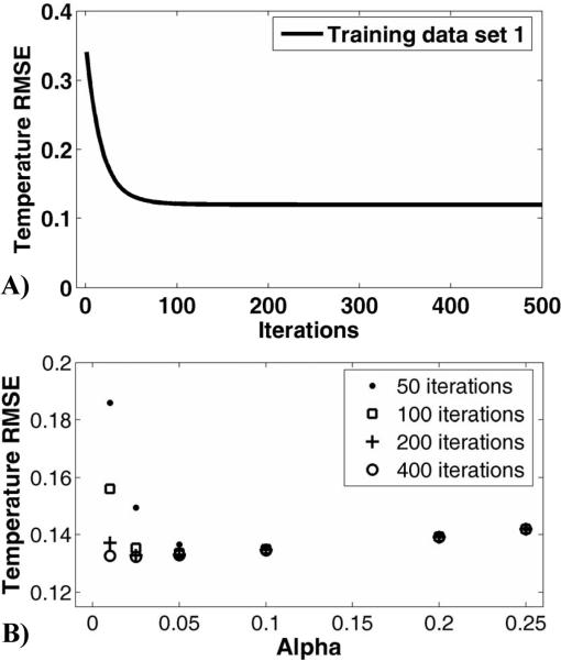
The TCR algorithm was optimized by first determining the α/iteration combination for all four parameter permutations in both heating experiment categories. Consider the case of the first training data set from the ex vivo porcine group at a reduction factor of four, using the maximum smoothness constraint and one “future” time frame. The behavior of the temperature RMSE of time frame 20 is plotted against number of iterations in Figure 1a for α=0.05. Beyond 200 iterations, little improvement is seen in the temperature RMSE. The RMSE values of this data set (now over all 60 time frames) for all α's at 50, 100, 200 and 400 iterations are shown in Figure 1B. The α/iteration combination that gave the lowest RMSE value was 0.025/400 (RMSE = 0.1322). The trend in the RMSE values for the second ex vivo porcine training data set was similar, although the minimum RMSE value was shifted out towards a higher alpha value: 0.20/400 (RMSE = 0.3169). For the two training data sets, using the optimal α at 100 iterations only degraded the temperature RMSE by 1.0% and 4.0%, respectively. Therefore, the number of iterations was set to 100 and a compromise value of α = 0.04 was chosen. The α/iteration combinations for the remaining permutations of algorithm parameters and the in vivo canine group were chosen in a similar fashion. The results are summarized in Table 1.

Fig 1.

Determining optimal values for α and number of iterations. A) The temperature RMSE of a single time frame from the first the ex vivo porcine training data set as a function of number of iterations. Convergence is almost complete after 100 iterations. B) The temperature RMSE for a number of different α/iteration combinations from the same data set.

Table 1.

α values, number of iterations, and temperature RMSE for all parameter sets. For the ex vivo porcine tissue case, the ex vivo training data sets were used to determine the α value and number of iterations. For the in vivo canine case, 2 sets of reconstructions were performed: one in which the in vivo training data was used to determine the α and iteration values (top rows) and one where the α and iteration values were taken from the ex vivo case (bottom rows). Only the validation data sets were used to determine the temperature RMSE.

	Ex vivo porcine tissue			In vivo canine
	α	iter	RMSE	α	iter	RMSE
Maximum smoothness, one “future” frame	0.04	100	0.26	0.05	200	0.82
				0.04	100	0.82
Maximum smoothness, no “future” frames	0.15	400	0.82	0.01	100	0.94
				0.15	400	0.95
Total variation, one “future” frame	0.0075	50	0.21	0.01	50	0.84
				0.0075	50	0.84
Total variation, no “future” frames	0.0035	400	0.27	0.005	100	0.94
				0.0035	400	0.97

Using the α/iteration combinations determined by the training data sets, the TCR algorithm was run to reconstruct the validation data sets in each experiment category for all parameter permutations (constraint type and whether or not to use one “future” time frame). Temperature RMSEs were calculated from the pooled voxels of all validation data sets for each category. The results are shown in Table 1. Two sets of results are shown for the in vivo canine experiments. In the top row, the α and iteration values were determined from the in vivo training data set. In the bottom row, the α and iteration values are those that were determined by the ex vivo training data sets. The top row RMSE results were used when comparing the different algorithm implementations for significant differences. For both experiment categories, the use of one “future” time frame in the reconstruction with a given constraint type led to significantly improved RMSE values (p < 0.05 for each). The total variation constraint performed significantly better than the maximum smoothness constraint in the ex vivo porcine tissue experiment category, but not in the in vivo canine category. The total variation constraint with one “future” time frame was chosen as the optimal parameter set because it required fewer iterations to converge. It should be noted that if using one “future” time frame in the reconstruction is not acceptable for a particular application, then the total variation constraint outperforms the maximum smoothness constraint significantly in the case the of ex vivo porcine tissue experiments (p <0.05) but not in the case of the in vivo canine experiments.

Maximum Reduction Factor

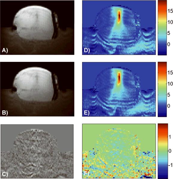
Using the optimized parameters of α = 0.0075, 50 iterations, the total variation constraint and the one “future” time frame in the TCR algorithm, the largest reduction factor achieved while keeping the temperature RMSE below 0.5°C was R=4 for the ex vivo porcine tissue experiment data sets. Magnitude images and temperature maps from time frame 16 of a validation data set are shown in Figure 2. Figure 2A shows a portion of the magnitude image reconstructed from the full data using the standard inverse Fourier Transform, while the image shown in Figure 2B was reconstructed using the TCR algorithm with R=4. The difference image is shown in Figure 2C, with a windowing that is 10 times narrower than the windowing used in A and B. There is no visible structure to the noise in the magnitude difference image. The corresponding temperature maps are shown in Figure 2D – E, with the temperature difference map scaled to show temperature differences from −2°C to 2°C. No structure can be seen in the temperature difference map around the region of the focal zone.

Fig 2.

Magnitude images and the corresponding temperature maps of time frame 16 of one ex vivo porcine tissue validation data set are shown. The full data are shown on top (A and D), TCR at R=4 is shown in the middle (B and E) and the difference images are shown on the bottom (C and F). The temperature difference map is scaled from −2°C to 2°C.

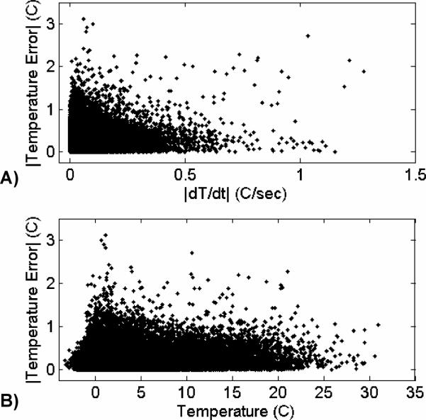
Because the constraint term in the TCR algorithm penalizes sharp changes in time, it was hypothesized that the largest errors would occur when the temperature was changing the most rapidly. To test this hypothesis, finite difference derivatives were calculated for the temperature-time curves of each voxel. A large ROI about the heated area was chosen and the absolute value of the temperature error of every voxel was plotted against the absolute value of its time derivative. This scatter plot, containing data from all six ex vivo porcine tissue validation data sets, is shown in Figure 3A. Contrary to the hypothesis, larger errors and faster changing temperatures are not correlated. Also of interest is the behavior of the algorithm as a function of temperature. A second scatter plot, shown in Figure 3B, shows the absolute value of the error plotted against temperature over the same ROI. The algorithms performance seems to be independent of temperature.

Fig 3.

A) Absolute value of temperature error plotted against the absolute value of dT/dt for all voxels in the heated region. Larger errors and faster changing temperatures are not correlated. B) Absolute value of temperature error plotted against temperature for all voxels in the heated region. Larger errors are higher temperatures are not correlated.

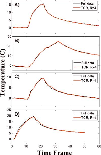
Four representative temperature versus time curves are shown in Figure 4. Each plot is of the voxel within the ultrasound focal zone that had the largest temperature change. The curve in Figure 4A is from the first training data set and the curves in Figures 4B – D are from validation data sets. The black lines show the temperatures calculated from the full data while the red lines show the temperatures calculated using TCR with R=4. In each case, the TCR temperatures do not deviate significantly from the full data temperatures. Even at times when the ultrasound power is turned on or off and the temperatures change abruptly, the TCR algorithm can handle these sharp changes. Although, the TCR temperatures plotted in Figure 4D do lag behind the full data temperatures slightly during heating and cooling. Also important to note is the ability of the TCR algorithm to accurately predict peak temperatures.

Fig 4.

Temperature versus time curves from the hottest voxels of four different ex vivo porcine tissue data sets. The TCR temperatures at R=4 agree quite well with the full data temperatures.

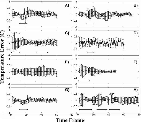
ROIs of approximately 5×10 voxels about the heated areas were chosen to obtain a more global sense of the algorithms performance. From these ROIs a mean and standard deviation of the error were calculated at each time frame. The results for all eight ex vivo porcine tissue data sets are displayed in Figure 5. The horizontal black bars below the error bars indicate the time frames during which heating was occurring. The plots in Figure 5A–F are the validation data sets and the remaining 2 plots are the training data sets. It can be seen that the mean error is zero for most time frames in most data sets and that the standard deviation of the error rarely rises above 0.5°C. On the occasions that the mean error deviates from zero, it does not differ by more than +/− 0.25°C. The one somewhat anomalous data set is the one shown in Figure 5D, as it exhibits peculiar periodic behavior. An artifact from the pulse sequence must have been present as the magnitude signal of this data set showed periodic fluctuations on the order of 5% in the non-heated region of the porcine tissue.

Fig 5.

The mean and standard deviation of temperature error for an ROI over the heated region shown at all time frames. A) through F) are ex vivo porcine tissue validation data sets and G) and H) are the training data sets. The horizontal bars represent times when the heating is on.

The largest reduction factor achieved with temperature RMSE less than 1.0°C for the canine data sets was R=3. Figure 6 shows the temperature maps of the canine training data set reconstructed with the full data and standard inverse Fourier Transform (A), with the TCR algorithm at R=3 (B), and the difference between the two scaled to +/− 2°C (C). Due to lower image signal to noise ratio (SNR) compared to the ex vivo porcine tissue experiments, the temperature maps for the canine experiments are relatively more noisy.

Fig 6.

A) Temperature map from in vivo canine data reconstructed with the full data. B) Same temperature map reconstructed with the TCR algorithm at R=3. C) Temperature difference map scaled from −2°C to 2°C.

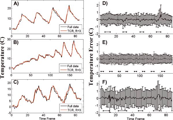
Temperature versus time curves from the three different experiments are shown in Figure 7A–C. Voxels from within the focal zone were chosen and the temperatures reconstructed from the full data (black lines) are compared against temperatures reconstructed from the TCR algorithm with R=3 (red lines). The plot shown in Figure 7A is the training data set. Despite the more noisy data, the TCR temperatures follow the full data temperatures fairly well. They are able to follow the abrupt rises in temperature at times when the ultrasound power is turned on. On a few occasions the TCR algorithm slightly under-predicts the peak temperatures, as in the last peaks in Figure 7B and C.

Fig 7.

A) through C): Temperature versus time curves for a voxel in the focal zone from the three in vivo canine data sets. The TCR temperatures at R=3 agree quite well with the full data temperatures. D) through F): The mean and standard deviation of temperature error for an ROI over the heated region from the same three data sets. D) is the training data set, E) and F) are the validation data sets. The horizontal bars represent times when the heating is on. The nosier canine data had a larger standard deviation than the ex vivo porcine tissue data sets, even at R=3.

The mean and standard deviation of the error from with an ROI about the region of heating is shown in Figure 7D–F for all three in vivo canine data sets. As with the ex vivo porcine tissue data sets, the mean error is very nearly zero for all time frames, deviating only occasionally to +/− 0.5°C. For these canine data sets, the standard deviation of the error is slightly higher than the porcine tissue data sets. In the first two sets it falls between +/− 0.5°C and +/− 1.0°C, while in the third set it regularly rises higher than +/−1.0°C.

Comparison to Sliding Window and Low Resolution Reconstructions

The TCR algorithm out performed the sliding window and low resolution reconstruction methods. The temperature RMSE values for the ex vivo porcine tissue data and in vivo canine data are shown in Table 2. A Fishers F-test confirmed that the TCR RMSE values from both experiment categories were significantly lower than the RMSE values from the sliding window reconstruction and low resolution reconstruction (p < 0.05 in all cases).

Table 2.

Temperature RMSE values for TCR algorithm, sliding window reconstruction and low resolution reconstruction.

	TCR	Sliding Window	Low Resolution
RMSE, Ex vivo porcine tissue	0.21	0.31	0.45
RMSE, In vivo canine	0.84	0.94	1.42

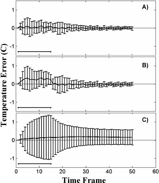
Figure 8 shows the mean and standard deviation of the temperature error over a small ROI about the focal zone for the three different reconstruction methods. The data is from an ex vivo porcine tissue validation data set and the time frames during which heating was occurring is shown by black horizontal lines. The TCR errors are shown in Figure 8A, sliding window errors in Figure 8B and low resolution errors in Figure 8C. The mean error of the sliding window reconstruction is greater than zero during all time frames when heating is on, indicating that this method systematically under-predicts temperature changes during heating. This effect is due to the fact that the sliding window method uses k-space data from previous time frames in the reconstruction and therefore the temperature measurements lag behind the actual temperatures. The low resolution reconstruction has a much larger standard deviation on the error and under-predicts the temperature through out the heating and cooling phases. While the TCR method shows slightly elevated mean errors during heating, they are not nearly to the extent of the sliding window errors. Additionally, the standard deviations of the TCR errors are smaller than the standard deviations of the errors of the other two techniques.

Fig 8.

Mean and standard deviation of temperature error over an ROI for an ex vivo porcine tissue validation data set. The TCR algorithm at R=4 is shown in A); the sliding window reconstruction in shown in B); and the low resolution reconstruction is shown in C).

Discussion

A temporally constrained reconstruction technique applied to undersampled PRF temperature data has been presented. The TCR method is an iterative technique that takes advantage of physically appropriate assumptions about the data in order to resolve the artifacts that normally occur when reconstructing undersampled data. In the work presented here, the assumption is that temperature changes are relatively smooth in time. For the ex vivo porcine tissue heating experiments, it has been shown that the TCR technique is capable of reconstructing PRF images using only 25% of the full data (R=4) without introducing significant error into the temperature information. For the in vivo canine experiments, where the pulsed heating at high ultrasound powers induced abrupt temperature changes and the SNR was significantly lower, the TCR technique reconstructed images with accurate temperature information using only 33% of the full data (R=3). At these reduction factors, the TCR reconstruction outperformed sliding window reconstruction and low resolution reconstruction in both heating experiment categories.

The TCR technique was tested with a number of variations to the algorithm. The method for choosing the optimal α and iteration values relied on the availability of the full data temperatures to be used as truth. In a real application this will not be the case, and L-curve analysis (18) would have to be used to determine α and some stopping criteria would have to be used to terminate the iteration process. However it should be noted that the performance of the algorithm is fairly stable over a range of α and iteration values. In Figure 1 it can be seen that at 200 iterations the RMSE does not change more than 5% over a range of α's from 0.01 to 0.2. For the case of the TCR algorithm that used the maximum smoothness constraint and no “future” time frames, where the optimal ex vivo and in vivo α values are quite different, the temperature RMSE of the two ex vivo training data sets only vary by 13% and 12% over a range of α's from 0.01 to 0.2. Also, a single α/iteration can be used across multiple data sets with similar results. The validation data sets that used α/iteration combinations chosen by the training data sets did not have significantly larger errors and the α/iteration values determined using the ex vivo porcine tissue group were very similar to those determined independently by the in vivo canine group.

An additional indication of the algorithm's robustness with respect to the α and iteration combination can be seen in the results presented in Table 1. When the in vivo canine validation data sets were reconstructed with the α and iteration values determined from the ex vivo porcine tissue data sets, the four RMSE values were different from the original RMSE values by 0.0%, 1.1%, 0.0%, and 3.2%, respectively. These small changes in the RMSE values indicate that the TCR algorithm is robust enough that the α and iteration parameters can be determined from ex vivo experiments and then used for in vivo applications. For a final test of robustness, the reconstruction of the in vivo canine validation data sets was done with the ex vivo porcine tissue α values and with the number of iterations fixed at 400. The RMSE values and percent changes were: 0.82 (0.0%), 0.95 (1.1%), 0.87 (3.6%), 0.97 (3.2%). Again, the small changes in RMSE values suggest that if computation time is not a concern, the number of iterations can be fixed at a single, relatively large number.

The TCR technique does not use any coil sensitivity information and could be used in conjunction with parallel imaging methods for even larger reduction factors. The data presented here was taken from one channel of a two-channel receive coil (the channel with the higher SNR was chosen). While parallel imaging methods produce images with reduced SNR, the TCR technique was found to not degrade the SNR of its reconstructed image. This is largely due to the fact that the algorithm smoothes the data in time and thus signal fluctuations in temporally-adjacent images are reduced.

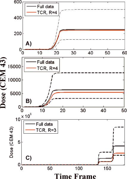
MR images can be used to monitor thermal therapies in a number of different ways. Modifications to the heating deposition can be made by a clinician or a controlling computer and such modifications can be based on either an end point temperature or an accumulated dose. It has been shown that the TCR algorithm predicts peak temperature quite well. The calculation of dose is extremely sensitive to temperature error at high temperatures due to the exponential relationship between the two. Figure 9 shows a comparison of dose calculations made with the full data and the TCR algorithm. Figure 9A shows the dose versus time curve for the voxel with the largest dose accumulation from the first ex vivo porcine tissue training data set. Figures 9B and C are similar plots from a validation ex vivo porcine tissue data set and a validation in vivo canine data set. The TCR algorithm under-predicts dose accumulation in all three instances. In addition to the voxels shown here, all voxels that received 240CEM of dose or greater were analyzed (if 240CEM was not achieved in a particular data set then the voxel with the largest dose was considered). It was found that the TCR algorithm consistently, although not always, under-predicted the thermal dose. Over all of these voxels, the average dose error was −6.3% for the ex vivo porcine tissue data sets and −28% for the in vivo canine data sets. The reason for these underestimations is that the constraint term in the TCR algorithm penalizes abrupt changes in time, causing the reconstructed temperatures to sometimes fall short at sharp peaks. This subtle smoothing of the temperature curves can be seen in the last peak of the temperature plot in Figure 7B. To put these errors into perspective, dashed black lines are shown on the plots in Figure 9 that represent the dose accumulation that would be calculated from the full data temperatures if there were a systematic temperature offset of +1°C or −1°C. This type of offset could occur, for example, if the subject body temperature was actually 38°C when it was assumed to be 37°C. Seen in this light, the TCR errors in calculating dose are reasonable.

Fig 9.

Dose versus time plots, comparing the TCR algorithm to the full data. The plots in A) and B) are from ex vivo porcine tissue data sets and the plot in C) is from an in vivo canine data set. The dashed black lines represent the dose that would be calculated from the full data if the temperatures were systematically shifted by +/− 1°C.

In its current form, the computation time for the TCR algorithm is still too long for real time image acquisition. In a Matlab (The Mathworks, Natick, MA, USA) implementation on a desktop PC, it takes approximately 5.7 seconds to reconstruct one slice using the total variation constraint and 50 iterations. Considering that 5 to 10 slices will have to be reconstructed in 1 or 2 seconds, the computation time will have to be improved by a factor of between 15 and 115. Several ideas will enable the reduction of the computation time to reach real-time. When passing the k-space data into the algorithm, one need only use a small number of data points in the readout direction, keeping only the central portion of the image where the heating is being monitored. This will not accelerate scan time at all, but it will reduce the size of the data matrix that goes into the reconstruction algorithm and lessen the computation burden. For all data sets, a quarter of the read out data was sufficient to still visualize the entire heated area. There will be no reduction in image resolution and since the entire readout data will have been acquired, it can be reconstructed retrospectively if necessary. Cutting the data matrix by a factor of four in the readout direction led to a four fold acceleration in the TCR algorithm. If some temperature accuracy can be sacrificed, then it would be possible to use the algorithm with a constraint weighting term that has been optimized for fewer iterations. Finally, an efficient C++ implementation on a more powerful computer that uses a conjugate gradient method to minimize the cost function, instead of the currently used gradient descent technique, will provide additional improvement in computation time. Recently published papers have shown that computationally intensive medical imaging tasks can be processed on a graphics processing unit (GPU) to increase computation speed by factors of 85 to 100 (23,24). On such a computer or other parallel computing platforms, real time implementation would be feasible.

Even greater reduction factors should be attainable with more sophisticated constraint terms. A number of investigators have shown reconstruction is possible using total variation in space as a constraint (25). These could be used in addition to the temporal constraint that is already implemented. We believe that information about tissue heating could also be incorporated into the constraint term. Heating start and stop times as well as ultrasound power will be known during any thermal treatment and the temperature evolution within the tissue will follow the Pennes bioheat equation. Using this a priori information to predict how the temperature, and thus the image phase, will behave could prove to be very useful in the reconstruction algorithm.

References

- 1.Bublik M, Sercarz JA, Lufkin RB, Masterman-Smith M, Polyakov M, Paiva PB, Blackwell KE, Castro DJ, Paiva MB. Ultrasound-guided laser-induced thermal therapy of malignant cervical adenopathy. Laryngoscope. 2006;116(8):1507–1511. doi: 10.1097/01.mlg.0000230403.13826.69. [DOI] [PubMed] [Google Scholar]
- 2.Fosse E. Thermal ablation of benign and malignant tumours. Minim Invasive Ther Allied Technol. 2006;15(1):2–3. doi: 10.1080/13645700500500862. [DOI] [PubMed] [Google Scholar]
- 3.Carter DL, MacFall JR, Clegg ST, Wan X, Prescott DM, Charles HC, Samulski TV. Magnetic resonance thermometry during hyperthermia for human high-grade sarcoma. Int J Radiat Oncol Biol Phys. 1998;40(4):815–822. doi: 10.1016/s0360-3016(97)00855-9. [DOI] [PubMed] [Google Scholar]
- 4.Denis de Senneville B, Quesson B, Moonen CT. Magnetic resonance temperature imaging. Int J Hyperthermia. 2005;21(6):515–531. doi: 10.1080/02656730500133785. [DOI] [PubMed] [Google Scholar]
- 5.Quesson B, de Zwart JA, Moonen CT. Magnetic resonance temperature imaging for guidance of thermotherapy. J Magn Reson Imaging. 2000;12(4):525–533. doi: 10.1002/1522-2586(200010)12:4<525::aid-jmri3>3.0.co;2-v. [DOI] [PubMed] [Google Scholar]
- 6.Sapareto SA, Dewey WC. Thermal dose determination in cancer therapy. Int J Radiat Oncol Biol Phys. 1984;10(6):787–800. doi: 10.1016/0360-3016(84)90379-1. [DOI] [PubMed] [Google Scholar]
- 7.Hazle JD, Stafford RJ, Price RE. Magnetic resonance imaging-guided focused ultrasound thermal therapy in experimental animal models: correlation of ablation volumes with pathology in rabbit muscle and VX2 tumors. J Magn Reson Imaging. 2002;15(2):185–194. doi: 10.1002/jmri.10055. [DOI] [PubMed] [Google Scholar]
- 8.Arora D, Minor MA, Skliar M, Roemer RB. Control of thermal therapies with moving power deposition field. Phys Med Biol. 2006;51(5):1201–1219. doi: 10.1088/0031-9155/51/5/011. [DOI] [PubMed] [Google Scholar]
- 9.Arora D, Cooley D, Perry T, Guo J, Richardson A, Moellmer J, Hadley R, Parker D, Skliar M, Roemer RB. MR thermometry-based feedback control of efficacy and safety in minimum-time thermal therapies: phantom and in-vivo evaluations. Int J Hyperthermia. 2006;22(1):29–42. doi: 10.1080/02656730500412411. [DOI] [PubMed] [Google Scholar]
- 10.Moonen CT, Liu G, van Gelderen P, Sobering G. A fast gradient-recalled MRI technique with increased sensitivity to dynamic susceptibility effects. Magn Reson Med. 1992;26(1):184–189. doi: 10.1002/mrm.1910260118. [DOI] [PubMed] [Google Scholar]
- 11.Mougenot C, Salomir R, Palussiere J, Grenier N, Moonen CT. Automatic spatial and temporal temperature control for MR-guided focused ultrasound using fast 3D MR thermometry and multispiral trajectory of the focal point. Magn Reson Med. 2004;52(5):1005–1015. doi: 10.1002/mrm.20280. [DOI] [PubMed] [Google Scholar]
- 12.Pruessmann KP, Weiger M, Scheidegger MB, Boesiger P. SENSE: sensitivity encoding for fast MRI. Magn Reson Med. 1999;42(5):952–962. [PubMed] [Google Scholar]
- 13.Sodickson DK, Manning WJ. Simultaneous acquisition of spatial harmonics (SMASH): fast imaging with radiofrequency coil arrays. Magn Reson Med. 1997;38(4):591–603. doi: 10.1002/mrm.1910380414. [DOI] [PubMed] [Google Scholar]
- 14.Madore B, Glover GH, Pelc NJ. Unaliasing by fourier-encoding the overlaps using the temporal dimension (UNFOLD), applied to cardiac imaging and fMRI. Magn Reson Med. 1999;42(5):813–828. doi: 10.1002/(sici)1522-2594(199911)42:5<813::aid-mrm1>3.0.co;2-s. [DOI] [PubMed] [Google Scholar]
- 15.Tsao J, Boesiger P, Pruessmann KP. k-t BLAST and k-t SENSE: dynamic MRI with high frame rate exploiting spatiotemporal correlations. Magn Reson Med. 2003;50(5):1031–1042. doi: 10.1002/mrm.10611. [DOI] [PubMed] [Google Scholar]
- 16.van Vaals JJ, Brummer ME, Dixon WT, Tuithof HH, Engels H, Nelson RC, Gerety BM, Chezmar JL, den Boer JA. “Keyhole” method for accelerating imaging of contrast agent uptake. J Magn Reson Imaging. 1993;3(4):671–675. doi: 10.1002/jmri.1880030419. [DOI] [PubMed] [Google Scholar]
- 17.Webb AG, Liang ZP, Magin RL, Lauterbur PC. Applications of reduced-encoding MR imaging with generalized-series reconstruction (RIGR) J Magn Reson Imaging. 1993;3(6):925–928. doi: 10.1002/jmri.1880030622. [DOI] [PubMed] [Google Scholar]
- 18.Adluru G, Awate SP, Tasdizen T, Whitaker RT, Dibella EV. Temporally constrained reconstruction of dynamic cardiac perfusion MRI. Magn Reson Med. 2007;57(6):1027–1036. doi: 10.1002/mrm.21248. [DOI] [PubMed] [Google Scholar]
- 19.Gamper U, Boesiger P, Kozerke S. Compressed sensing in dynamic MRI. Magn Reson Med. 2008;59(2):365–373. doi: 10.1002/mrm.21477. [DOI] [PubMed] [Google Scholar]
- 20.Adluru G, Whitaker RT, DiBella EVR. Spatio-Temporal Constrained Reconstruction of sparse Dynamic Contrast Enhanced Radial MRI Data. IEEE International Symposium on Biomedical Imaging.2007. pp. 109–112. [Google Scholar]
- 21.De Poorter J, De Wagter C, De Deene Y, Thomsen C, Stahlberg F, Achten E. Noninvasive MRI thermometry with the proton resonance frequency (PRF) method: in vivo results in human muscle. Magn Reson Med. 1995;33(1):74–81. doi: 10.1002/mrm.1910330111. [DOI] [PubMed] [Google Scholar]
- 22.Hindman JC. Proton Resonance Shift of Water in the Gas and Liquid States. The Journal of Chemmical Physics. 1966;44(12) [Google Scholar]
- 23.Hansen MS, Atkinson D, Sorensen TS. Cartesian SENSE and k-t SENSE reconstruction using commodity graphics hardware. Magn Reson Med. 2008;59(3):463–468. doi: 10.1002/mrm.21523. [DOI] [PubMed] [Google Scholar]
- 24.Sorensen TS, Schaeffter T, Noe K, Hansen MS. Accelerating the Nonequispaced Fast Fourier Transform on Commodity Graphics Hardwar. IEEE Transactions on Medical Imaging. 2008;27(4):538–547. doi: 10.1109/TMI.2007.909834. [DOI] [PubMed] [Google Scholar]
- 25.Block KT, Uecker M, Frahm J. Undersampled radial MRI with multiple coils. Iterative image reconstruction using a total variation constraint. Magn Reson Med. 2007;57(6):1086–1098. doi: 10.1002/mrm.21236. [DOI] [PubMed] [Google Scholar]