Tolerance adaptation and precipitation changes complicate latitudinal patterns of climate change impacts

Abstract

Global patterns of biodiversity and comparisons between tropical and temperate ecosystems have pervaded ecology from its inception. However, the urgency in understanding these global patterns has been accentuated by the threat of rapid climate change. We apply an adaptive model of environmental tolerance evolution to global climate data and climate change model projections to examine the relative impacts of climate change on different regions of the globe. Our results project more adverse impacts of warming on tropical populations due to environmental tolerance adaptation to conditions of low interannual variability in temperature. When applied to present variability and future forecasts of precipitation data, the tolerance adaptation model found large reductions in fitness predicted for populations in high-latitude northern hemisphere regions, although some tropical regions had comparable reductions in fitness. We formulated an evolutionary regional climate change index (ERCCI) to additionally incorporate the predicted changes in the interannual variability of temperature and precipitation. Based on this index, we suggest that the magnitude of climate change impacts could be much more heterogeneous across latitude than previously thought. Specifically, tropical regions are likely to be just as affected as temperate regions and, in some regions under some circumstances, possibly more so.

In his widely influential paper Evolution in the Tropics, Theodosius Dobzhansky (1) observed that “changeable environments put the highest premium on versatility rather than on perfection in adaptation.” If temperate populations experience greater variation in temperature compared with tropical populations, he predicted that those populations would have relatively greater versatility or be better adapted to variation in temperature. Put another way, populations should have a wider thermal tolerance in temperate climates. Janzen (2) famously extended this logic to an altitudinal gradient suggesting that tropical populations, adapted to relatively narrow variation in temperature, would be more spatially constrained and that “mountain passes” may actually be physiologically higher in the tropics. Results from studies testing Janzen's hypothesis generally support the theory, although caveats and exceptions certainly exist (3).

Models of evolution in changing environments often start from this “jack-of-all-trades is a master of none” premise (4, 5) and mathematically structure the “versatility” rather than “perfection” argument of adaptation to environmental variation. Specialization to one environment assumes a cost of adaptation to multiple environments such that a tradeoff is fundamental to modeling generalist–specialist evolution (6). In nature, local adaptation to native environmental conditions encountered throughout a lifetime is common although the tradeoffs and costs of adaptation to other environments are often weak (7). However, this intuitive and tractable concept has gained popularity in models as a starting point for understanding evolution in changing environments despite the many demonstrated exceptions to the “jack-of-all-trades is a master of none” tradeoff (5, 8).

To examine the implications of this versatility pattern for the study of global climate change, Deutsch et al. (9) analyzed empirical thermal performance curves of ectotherms on a latitudinal gradient. Their data supported the claim that ectotherms have a smaller thermal breadth in the tropics and furthermore found that based on climate change projections for the year 2100 (10), tropical ectotherms would be more adversely impacted in the future than temperate ectotherms despite the greater magnitude of change in climate expected at the poles.

Temporal scale is an essential component of models of evolution in changing environments. Although some evolution is likely to take place in between the present climate conditions and projected future climate conditions, and indeed has for many species in past historical climate change events, the extremely rapid nature of our current climate crisis could make adaptation difficult (11, 12). The performance breadth (specialist vs. generalist) of a population along with the rate of climate change determines the population's ability to adapt to the climatic change. In the face of rapid climate change, extreme specialists face a high threat of extinction but extreme generalists have a diminished capacity to adapt to changing climates due to relatively weak forces of stabilizing selection (13). When performance breadth and maximum performance tradeoffs exist (versatility vs. perfection), the strength of stabilizing selection is even weaker such that specialists, while still facing a high threat of extinction, are more favored evolutionarily than if there is no tradeoff (13).

Spatial heterogeneity is also a critical component. Greater variation in spatial heterogeneity tends to a wider environmental tolerance (14, 15). This can happen either through greater dispersal capacity of an organism leading to a wider variety of environmental variation experienced or through increased topographic diversity in a given habitat. Tropical ecosystems have a shallow latitudinal gradient in temperature (i.e., spatial heterogeneity is more homogenized) that makes it difficult for organisms to shift ranges poleward because they have to move much farther latitudinally to experience the same change in temperature compared with temperate organisms (16). Mountainous regions with greater topographic and altitudinal diversity are subject to a lower “climate change velocity,” and species in these regions will be better able to escape the effects of climate change vertically (17). However, in the absence of mountains, the low spatial heterogeneity of climate experienced in the tropics exacerbates climate change effects twofold: (i) by encouraging narrow environmental tolerance adaptation and (ii) by increasing the difficulty in matching changes in climate by moving latitudinally.

However, temperature is not the only important climatic variable affecting populations, and as Dobzhansky (1) also noted, “the widespread opinion that seasonal changes are absent in the tropics is a misapprehension.” Precipitation varies a great deal within a year in many regions of the tropics and, in fact, overall precipitation exhibits greater seasonality in the tropics compared with the higher latitudes (18). Although precipitation is predicted to change in many regions of the world (10), we have little understanding of how alteration of precipitation regimes will affect biodiversity. This is primarily because it is much less clear how variation in precipitation affects fitness of an organism than it is how temperature changes impact an organism's fitness (19). Furthermore, even the projections for changes in precipitation are less certain than they are for temperature (10). Predictions of how changes in precipitation will affect populations globally remain a significant gap in our understanding of climate change effects on biodiversity.

Here, we apply the model of environmental tolerance evolution of Lynch and Gabriel (14) to global climate data and then use the resulting tolerance breadth results to predict relative changes in fitness to populations across the globe based on climate change projections for 2100. We compare the results for temperature changes to Deutsch et al. (9) and extend the model to precipitation data to see which regions might be more vulnerable to changes in precipitation. Finally, we adapt the regional climate change index (RCCI) of Giorgi (20) to include the effects of environmental variation and tolerance adaptation. Our results have important implications for the potential global impacts of climate change and emphasize that (i) the evolutionary histories of populations are a critical consideration in assessing climate change vulnerability and (ii) precipitation changes resulting from climate change could have significant impacts on global biodiversity. The results are discussed in the context of current efforts to assess species extinction threats and vulnerability to global climate change.

Results

The model of tolerance adaptation behaved as predicted such that populations living at high latitudes (northern hemisphere specifically) with high thermal seasonality had wider performance breadths but lower fitness peaks than tropical, low-seasonality environments (Fig. 1). Therefore, the model exhibits a versatility vs. perfection tradeoff in the face of annual environmental variation.

Fig. 1.

Fitness curve model output with Alaskan (σ = 11.60 °C) and Central American (σ = 3.12 °C) seasonality inputs.

We found a very clear increase in temperature seasonality with increasing latitude in the northern hemisphere whereas the southern hemisphere, though following the same trend, was less severe in steepness (Fig. 2A). The northern hemisphere also follows a clear warming prediction of greater impact at higher latitudes compared with lower latitudes (Fig. 2C). The coefficient of variation for precipitation is highest at lower latitudes trending toward lower seasonality at the poles, although there is significant scatter particularly in the northern hemisphere (Fig. 2B). Changes in precipitation, like temperature, appear to amplify at higher latitudes but only in the northern hemisphere (Fig. 2D).

Fig. 2.

Latitude and seasonal variation in temperature (A) and precipitation (B) (based on 1961–1990 CRU climate data). Latitude and both RWAF (regional warming amplification factor) (C) and RPCF (regional precipitation change factor) (D) based on IPCC emission scenarios for 2080–2099. Open circles/dotted lines are dry-season values, and filled circles/solid lines represent wet-season values.

The combination of the tolerance breadth as predicted by seasonality along with projected temperature and precipitation changes results in a complicated picture regarding relative fitness changes across latitude. Fitness changes resulting from warming are clearly highest in the tropics compared with higher latitudes because of the lower thermal tolerance breadth resulting from low thermal seasonality (Fig. 3A). The pattern is very similar to the results of Deutsch et al. (9), who also found the highest impacts of warming on ectotherms to be concentrated in the tropics (figure 1C in ref. 9). Fitness changes resulting from precipitation loss and gains are not so clearly distributed across latitude but show the greatest impact on biotas in high-latitude northern regions and the smallest impact on biotas in high-latitude southern regions (Fig. 3B). Tropical regions show varied responses. This probably results from the greater scatter in both seasonality and precipitation changes observed across latitude (Fig. 2).

Fig. 3.

Relative change in fitness among global regions based on temperature (A) and precipitation (B) seasonality and projected change.

Changes in fitness from warming and precipitation change as well as projected magnitude change in the interannual variability of temperature and precipitation are all cumulatively estimated by the ERCCI (Fig. 4 and Table S1). The Mediterranean (MED) and Southern Equatorial Africa (SQF) are projected to be the hardest hit regions. Next, Central America (CAM), Northern Europe (NEU), Northeastern Europe (NEE), Southeast Asia (SEA), and West Africa (WAF) are also likely to be highly impacted by global climate change.

Fig. 4.

ERCCI (evolutionary regional climate change index) projection with larger circles (higher ERCCI values) representing greater predicted impact as a linear function of fitness changes from precipitation and temperature change and changes in the variability of temperature and precipitation. The index is relative such that comparisons can be made between regions but the magnitude is unknown and dependent on a variety of factors including future emissions—i.e., a small circle does not suggest that there will be small impacts in a given region, only that the impacts are projected to be smaller for that region compared with a region with a larger circle.

Discussion

The results further emphasize that the magnitude of change in an environmental variable is not the only determining factor in species’ responses to climate change: their evolutionary histories, and particularly their sensitivities to those variables, must also be incorporated (5, 9, 21, 22). In the case of temperature, the tolerance evolutionary model predicts stronger impacts of climate change to tropical organisms as predicted by previous global change models (9). As for precipitation, however, evolutionary models of sensitivity have not been developed despite its ecological and evolutionary importance. In our application of the tolerance adaptation model to precipitation data, we found that although high-latitude northern hemisphere regions will be most heavily impacted by future climate change, many lower latitude, tropical regions will also be strongly impacted. The results also emphasize hemispheric asymmetry (23), and that even though the southern hemisphere is generally less climatically variable (Fig. 2), the magnitude changes in temperature and precipitation make some regions in the southern hemisphere relatively vulnerable (Fig. 4).

The structure of the tolerance adaptation model we used, developed by Lynch and Gabriel (14), is a straightforward optimality model based on the “jack-of-all-trades is a master of none” premise. However, many exceptions to this assumption are found in nature (5, 8). Other assumptions have the potential to complicate conclusions derived from the model. For example, when changes in fitness are accumulated additively through changes in fertility as in the model by Gilchrist (15), rather than survivorship as in Lynch and Gabriel (14), the conclusions can be quite different. Gilchrist (15) predicts that more important than within-generation environmental heterogeneity (in this model, thermal heterogeneity specifically) is the relationship between the within- and among-generation environmental heterogeneity (5). In addition, Gilchrist (15) models the performance curve as a more realistic asymmetric thermal performance function with a more rapidly decreasing fitness in hot environments. Despite these simplifying assumptions, we have reason to believe that the tolerance adaptation model reasonably approximates thermal performance curves at least at a global scale. Our fitness change results (Fig. 3A) are remarkably consistent with the results of Deutsch et al. (9), who derived thermal performance curves from empirically collected insect laboratory and population data and also found a strong signal of greater climate change impacts in tropical latitudes. One notable departure from our analysis is that because Deutsch et al. (9) have insect population data, their changes in fitness are quantifiable (as measured by population growth), whereas the changes in fitness we measured from the model are strictly relative and the values for any region are meaningless when taken out of the context of global comparison.

Because the tolerance adaptation model of Lynch and Gabriel (14) is so general, we can also apply it to precipitation data. The pattern in fitness changes from precipitation changes is not as clear as that found from temperature changes. However, it appears that both the low seasonality in precipitation at high latitudes in the northern hemisphere along with the large magnitude changes in precipitation projected could threaten the populations that live there (Fig. 3B). These results are consistent with the prediction that species at high latitudes might be heavily impacted by the relatively greater changes in precipitation in these regions seen in global change models (24). Additionally, however, our model suggests that many tropical regions (Table S1) could also be strongly impacted and highlight the greater scatter in results found from precipitation changes as compared with temperature changes.

Precipitation variables (along with temperature) are commonly used in “climate envelope” modeling efforts examining large-scale climate change effects on species (for examples see refs. 25 and 26). Envelope models are useful but neglect, among other things, past and future adaptation to climatic variability (27). Our approach incorporates adaptation to annual variation in precipitation (and temperature) and examines how different tolerance breadths alter predictions of geographic impacts of climate change. Empirical support is lacking for the evolutionary consequences of precipitation variability and climate change implications. In an exemplary and comprehensive review of responses to recent climate change, Parmesan (28) mentions “precipitation” once, “rainfall” twice, and “temperature” 46 times. Despite this, we know rainfall can be a strong selective force often acting indirectly to influence habitat structure, food supply, and resource availability (29, 30). Moreover, there is some evidence to suggest that species might experience local adaptation to precipitation regimes in a Gaussian manner, as we have modeled. For example, changes in rainfall variability (too many high- and low-rainfall years) was the primary factor in the decline and eventual extirpation of the well studied bay checkerspot butterfly (Euphydryas editha bayensis) population of the Jasper Ridge Biological Preserve in California (31). More data and theory are needed, however, as has been developed for thermal adaptation (5) to conclusively validate this aspect of this model. Nevertheless, the Lynch and Gabriel (14) model we have applied to precipitation is consistent with generalist/specialist tradeoff theory and does provide one hypothesis as to how variation in rainfall could structure “precipitation performance curves.”

Further caveats are critical to consider when interpreting the results of this analysis. First, for reasons of tractability, we used a very large spatial scale of climatic variation that is unlikely to match the range of individual organisms. Ideally, we would rather not average over regions as different as Rocky Mountain West and Southern California because populations are likely responding to climatic variation at much smaller spatial scales. However, to a first approximation, we feel that this scale is still informative and that it does capture some of the regional variability important to evolutionary processes. Second, we also simplified significantly the temporal variation likely influencing tolerance adaptation. In our application of the model, we take two static points in time: the “naturally” variable period of 1961–1990 and the climatic conditions projected for 2088–2099. In reality, each of these time periods are likely subject to dynamic variation in climate—rising average temperature, for example—that could have important eco-evolutionary consequences. In addition, if rates of evolution vary geographically, then that could also affect projections of climate change impacts across latitude. In the case of Drosophila, the genetic variance in traits for environmental tolerance is lower for tropical species (32). Low levels of genetic variability in tropical populations may hamper their abilities to adapt to changing climatic conditions and could compound the effects that we have examined regarding narrow tolerance range.

The ERCCI we have formulated based on the magnitude change-focused RCCI of Giorgi (20) gives similar results as the RCCI but differs significantly in many ways. First, the ERCCI incorporates changes in fitness using a general adaptive model so that the values of the ERCCI are relevant to changes in populations and species (and biodiversity, which is ultimately a function of species and populations). The RCCI is less restrictive in that it is only a function of changes in the mean and variability of temperature and precipitation, and could be more applicable to, for example, human systems (which may significantly violate many of the ERCCI assumptions we have outlined).

In both the RCCI and ERCCI indices, the region most vulnerable to climate change is the Mediterranean where the magnitude change and change in the variability of both precipitation and temperature are projected to be high. In addition, both indices suggest that Northern Europe and Central America are both highly vulnerable. However, the ERCCI suggests that Southern Equatorial Africa may be, along with the Mediterranean, among the most heavily impacted regions. Additionally, Southeast Asia and West Africa appear to be highly vulnerable to climate change effects more so than predicted by Giorgi (20). The elevation in threat level of these regions using the ERCCI is due to the incorporation of tolerance adaptation, which represents an important consideration when examining the relative impacts of global climate change. However, the ERCCI should not be taken as a literal mapping of global vulnerability to climate change. There are many factors that go into determining species vulnerability—including microhabitat, behavior, biotic interactions, genetic diversity, etc. (21)—that we have not considered here. In fact, although the generality and non-taxon–specific nature of this analysis increases its applicability to systems, it also decreases the accuracy of individual predictions. What our results do suggest, however, is that incorporating seasonality and environmental variation in an adaptive context produces a very heterogeneous picture of climate change impacts across latitude.

Predicting the impacts of climate change on global biodiversity will require a multitude of perspectives and approaches. Here, we have taken a first step and laid out a general framework for the relationship between environmental variation and tolerance adaptation and its implication for global climate change impacts. Recent studies have demonstrated the high vulnerability of tropical organisms to global warming (5, 9, 16, 32), and this study provides an adaptive explanation for these patterns within an evolutionary modeling framework. Moreover, adaptation to precipitation variability and future projections of precipitation patterns further complicate the geographical pattern of climate change impacts compounding the already significant uncertainty in precipitation projections (10). These results together emphasize that we should carefully evaluate all of these components of vulnerability before assessing the impacts of projected climate change on species. In particular, it may be overly simplistic to state that “species at high latitudes will be most vulnerable to climate change” or that “tropical species will be the most heavily impacted” without full examination of the climatic and biological factors that determine vulnerability.

Materials and Methods

Model: Tolerance Adaptation.

We use the model of Lynch and Gabriel (14) based on a Gaussian distribution where z represents a phenotype over a gradient of a given environmental variable φ. More specifically, fitness over the variable φ is modeled as a Gaussian function with variable z₁ defined as the environmental optimum and z₂ as the performance breadth.

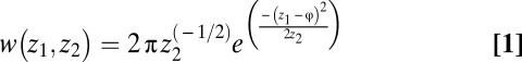We are interested in the relationship between within-generation variance in φ () and the optimal performance breadth. To find this relationship, Lynch and Gabriel (14) and Gabriel and Lynch (33) make simplifying assumptions so that this relationship can be analytically derived.

First, the phenotype z is an additive function of both genotypic (g) and environmental (or developmental) contributions (e). Thus, the expected value of the environmental variable is zero and the distribution of the environmental contribution is independent of the distribution of the genetic variable such that z₁ = g₁ + e₁ and z₂ = g₂ + e₂. Lynch and Gabriel (14) then derive a close approximation of the genotypic tolerance curve as a function of g₁, φ, and V, where V is defined as a linear combination of g₂ and the variances of e₁ and e₂. Second, it is assumed that within-generation variation in φ affects the genotypic tolerance curve arithmetically over space and geometrically through time. So the spatial distribution of φ experienced by an organism in its lifetime is defined as φ_s, and φ_t is defined as the within-generation (assuming discrete generations) distribution of φ. The variances are defined as and , respectively, by Lynch and Gabriel (14). Third, to determine the long-term geometric-mean fitness across generations, Lynch and Gabriel (14) incorporate the between-generation fitness, or . This model assumes that survivorship to reproduction is the product of survivorship at each time period (5). Lynch and Gabriel (14), therefore, take the limit approaching infinity of the product of the genotypic tolerance curve (w(g₁, g₂|φ_t)) to obtain Eq. 2.

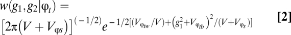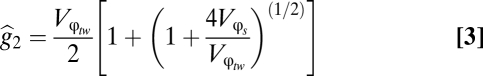
To derive the solution for optimal g₂, or , from Eq. 2, Gabriel and Lynch (33) assume negligible developmental noise (i.e., e₁ and e₂ are equal to 0). They also make the assumption that and are additive and that between-generation variance is negligible () to derive the final solution for .

Therefore, in this application of the Lynch and Gabriel model (14) we make several simplifying assumptions including (but not limited to) symmetric performance curves, no phenotypic plasticity or acclimation, and a “versatility/perfection” or “jack-of-all-trades is a master of none” tradeoff. These assumptions are often violated in nature (5). However, this analysis provides a first cut examination at how climatic variability might structure adaptation and, in turn, responses to environmental change, with explicit acknowledgment of the limitations (summarized above and detailed in refs. 5, 14, and 33).

Global Climate: Historical Variation and Change Projections.

We used a high-resolution interpolated 0.5° grid from Mitchell and Jones (34) that covers the global land surface (data available at www.ipcc-data.org/obs/cru_ts2_1.html). For historical variation in global climate, we used monthly means of temperature and precipitation averaged over the period from 1961 to 1990. To facilitate the analysis and interpretation, we aggregated averages over the 26 climatological regions defined by Giorgi and Bi (35). This scale is appropriate for our purposes precisely because we are interested in large-scale global patterns. For each region, we averaged both temperature and precipitation over all points in the grid. We also took the SD for each point and set of monthly temperature and precipitation values and then found the average SD for each region.

For climate change projections, we used the forecasts of Giorgi (20), allowing for comparison of our results to his assessment of global “climate change hot-spots.” Using the same regions as Giorgi and Bi (35), Giorgi (20) calculated modeled changes in temperature and precipitation from the period 1960–1979 to the period 2080–2099 averaged over the A1B, A2, and B1 IPCC emission scenarios (10). Giorgi (20) also split each region into two temporal periods, a wet season and a dry season, and calculated differences in precipitation and temperature for each season. These climate change projections were an aggregation of 20 climatic models and three IPCC emissions scenarios (A1B, A2, and B1) that encompass most of the climatic space explored by the IPCC (20). However, individual climate models and emission scenarios can have widely different results in terms of temperature and precipitation changes. Using the Giorgi (20) aggregations furthermore assumes that each scenario and model has an equal likelihood of occurring. Yet, such an assumption masks much of the uncertainty behind the models and scenarios (36). Particularly for precipitation changes, different climatic models often disagree in some regions even as to the sign of change although some regions have very good model agreement; for example, most models predict extensive drying in the Mediterranean (10). Although the relative nature of our analysis is likely robust to this essential point, we emphasize that populations will respond differently in absolute terms to different predictions of the models and emission scenarios. For example, a low CO₂ emissions scenario (e.g., B1) will have smaller impacts than a high-emissions scenario (e.g., A2), but both scenarios will likely have similar relative global impacts—the point of concern here.

Estimating Change in Relative Fitness.

To estimate the change in relative fitness for biotas in each global region, we applied the global climate data to the model of tolerance adaptation. Although the model of tolerance adaptation is very general, we must make further assumptions regarding the species of interest for which the data are easily applicable. Primarily, for annual organisms, , or the within-generation variance the organism experiences, is equal to the annual mean environmental value and its annual mean SD in each region. For simplicity, we assume a constant for the spatial heterogeneity of the environmental variable such that . Using Eq. 3, we can then solve for , the key “breadth” parameter for change in fitness. Because we are interested in the change in the environmental variable (φ), we assume g₁ = 0 and use Eq. 2 to calculate the change in fitness setting and the variances of e₁ and e₂ to a constant 1.

For the temperature data, we use the intraannual SD of temperature as and the RWAF (regional warming amplification factor) defined in Giorgi (20) as the φ in Eq. 2. We can then solve for w(g₁, g₂|φ) from Eq. 2. We also find w(g₁, g₂|φ) from Eq. 2 when φ = 0 and find the difference between the two values of w. This yields a change in fitness relative to other regions (Δw_t) based on both, the breadth of adaptation (g₂) and the change in temperature (RWAF). For comparative purposes, we also multiply the resulting value by 100 to get the final value of Δw_t; because Δw_t is unitless, we are only focusing on the changes in fitness relative to other regions. For precipitation, we define as the coefficient of variation (SD/mean) of the interannual monthly values. Using the coefficient of variation (rather than SD) provides a value of precipitation variability independent of the mean (20). Change in precipitation is measured by Giorgi (2006) as the percent change of the mean. We created a variable similar to the RWAF for precipitation by dividing the percent change in precipitation by the overall average change in precipitation. We multiplied this value by 10 for scaling purposes. This produced a regional precipitation change factor (RPCF), which we used as the deviation from g₁ or φ to find the change in fitness. We multiplied this change in fitness value by 10 (to scale to Δw_t) to get the final Δw_p value. We calculated Δw_p and Δw_t for both the dry season and the wet season. To examine latitudinal trends and plot latitude vs. change in fitness, we took the average change in fitness for both seasons and used the latitudinal midpoint for each region.

The regional climate change index (RCCI) developed by Giorgi (20) also takes into account regional changes in the interannual variability of both temperature and precipitation, as well as the magnitude change in the mean. Although this could be incorporated into an adaptive tolerance model, that is not the focus of the model we have applied, and so we explore the possible effects of variability changes indirectly. Following Giorgi (20), we created an evolutionary regional climate change index (ERCCI) by incorporating the wet- and dry-season changes in relative fitness, we calculated for both temperature (Δw_t) and precipitation (Δw_p) with the changes in regional interannual temperature and precipitation variability (Δσ_t and Δσ_p, respectively) calculated by Giorgi (20).

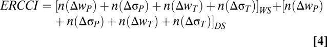For the value of the factor n, we follow table 1 of Giorgi (20) for and . For temperature, we use n = 0 for Δw_t < 0.5, n = 1 for 0.5 < Δw_t < 1, n = 2 for 1 < Δw_t < 1.5, and n = 4 for Δw_t > 1.5. For precipitation, we use n = 0 for Δw_p < 1, n = 1 for 1 < Δw_p < 1.5, n = 2 for 1.5 < Δw_p < 2.0, and n = 4 for Δw_p > 2.0. Therefore, the index provides a rough additive quantification of the relative effects of temperature and precipitation changes (and of the changes in variability of temperature and precipitation). Note that the index reflects subjectively chosen thresholds for n and more heavily weighs large impacts (20). For example, the dry-season change in fitness as a function of temperature for Central America (CAM) is 1.03, giving an ERCCI factor n of 2. For Southern Equatorial Africa (SQF), this change is 1.56 with n = 4 such that a doubling of the ERCCI factor does not necessarily indicate a doubling in the change of fitness (Table S1).

References

- 1.Dobzhansky T. Evolution in the tropics. Am Sci. 1950;38:209–221. [Google Scholar]
- 2.Janzen DJ. Why mountain passer are higher in the tropics. Am Nat. 1967;101:203–249. [Google Scholar]
- 3.Ghalambor CK, Huey RB, Martin PR, Tewksbury JJ, Wang G. Are mountain passes higher in the tropics? Janzen's hypothesis revisited. Integr Comp Biol. 2006;46:5–17. doi: 10.1093/icb/icj003. [DOI] [PubMed] [Google Scholar]
- 4.Levins R. Evolution in Changing Environments: Some Theoretical Explorations. Princeton: Princeton Univ Press; 1968. [Google Scholar]
- 5.Angilletta MJ. Thermal Adaptation: A Theoretical and Empirical Synthesis. Oxford: Oxford Univ Press; 2009. [Google Scholar]
- 6.Futuyma DJ, Moreno G. The evolution of ecological specialization. Annu Rev Ecol Syst. 1988;19:203–233. [Google Scholar]
- 7.Hereford J. A quantitative survey of local adaptation and fitness trade-offs. Am Nat. 2009;173:579–588. doi: 10.1086/597611. [DOI] [PubMed] [Google Scholar]
- 8.Huey RB, Hertz PE. Is a jack-of-all-trades a master of none? Evolution. 1984;38:441–444. doi: 10.1111/j.1558-5646.1984.tb00302.x. [DOI] [PubMed] [Google Scholar]
- 9.Deutsch CA, et al. Impacts of climate warming on terrestrial ectotherms across latitude. Proc Natl Acad Sci USA. 2008;105:6668–6672. doi: 10.1073/pnas.0709472105. [DOI] [PMC free article] [PubMed] [Google Scholar]
- 10.IPCC. Climate Change 2007: The Physical Science Basis. Contribution of Working Group I to the Fourth Assessment Report of the IPCC. Cambridge: Cambridge Univ Press; 2007. [Google Scholar]
- 11.Davis MB, Shaw RG. Range shifts and adaptive responses to Quaternary climate change. Science. 2001;292:673–679. doi: 10.1126/science.292.5517.673. [DOI] [PubMed] [Google Scholar]
- 12.Visser ME. Keeping up with a warming world; assessing the rate of adaptation to climate change. Proc Biol Sci. 2008;275:649–659. doi: 10.1098/rspb.2007.0997. [DOI] [PMC free article] [PubMed] [Google Scholar]
- 13.Huey RB, Kingsolver JG. Evolution of resistance to high temperature in ectotherms. Am Nat. 1993;142:S21–S46. [Google Scholar]
- 14.Lynch M, Gabriel W. Environmental tolerance. Am Nat. 1987;129:283–303. [Google Scholar]
- 15.Gilchrist GW. Specialists and generalists in changing environments. I. Fitness landscapes of thermal sensitivity. Am Nat. 1995;146:252–270. [Google Scholar]
- 16.Colwell RK, Brehm G, Cardelús CL, Gilman AC, Longino JT. Global warming, elevational range shifts, and lowland biotic attrition in the wet tropics. Science. 2008;322:258–261. doi: 10.1126/science.1162547. [DOI] [PubMed] [Google Scholar]
- 17.Loarie SR, et al. The velocity of climate change. Nature. 2009;462:1052–1055. doi: 10.1038/nature08649. [DOI] [PubMed] [Google Scholar]
- 18.Vázquez DP, Stevens RD. The latitudinal gradient in niche breadth: Concepts and evidence. Am Nat. 2004;164:E1–E19. doi: 10.1086/421445. [DOI] [PubMed] [Google Scholar]
- 19.Schneider SH, Root TL. Wildlife Responses to Climate Change: North American Case Studies. Washington, DC: Island; 2001. [Google Scholar]
- 20.Giorgi F. Climate change hot-spots. Geophys Res Lett. 2006;33:L08707. [Google Scholar]
- 21.Williams SE, Shoo LP, Isaac JL, Hoffmann AA, Langham G. Towards an integrated framework for assessing the vulnerability of species to climate change. PLoS Biol. 2008;6:2621–2626. doi: 10.1371/journal.pbio.0060325. [DOI] [PMC free article] [PubMed] [Google Scholar]
- 22.Kingsolver JG. The well-temperatured biologist. Am Nat. 2009;174:755–768. doi: 10.1086/648310. [DOI] [PubMed] [Google Scholar]
- 23.Chown SL, Sinclair BJ, Leinaas HP, Gaston KJ. Hemispheric asymmetries in biodiversity—A serious matter for ecology. PLoS Biol. 2004;2:1701–1707. doi: 10.1371/journal.pbio.0020406. [DOI] [PMC free article] [PubMed] [Google Scholar]
- 24.Walther G-R, et al. Ecological responses to recent climate change. Nature. 2002;416:389–395. doi: 10.1038/416389a. [DOI] [PubMed] [Google Scholar]
- 25.Thomas CD, et al. Extinction risk from climate change. Nature. 2004;427:145–148. doi: 10.1038/nature02121. [DOI] [PubMed] [Google Scholar]
- 26.Schröter D, et al. Ecosystem service supply and vulnerability to global change in Europe. Science. 2005;310:1333–1337. doi: 10.1126/science.1115233. [DOI] [PubMed] [Google Scholar]
- 27.Pearson RG, Dawson TP. Predicting the impacts of climate change on the distribution of species: Are bioclimate envelope models useful? Glob Ecol Biogeogr. 2003;12:361–371. [Google Scholar]
- 28.Parmesan C. Ecological and evolutionary responses to recent climate change. Annu Rev Ecol Syst. 2006;37:637–669. [Google Scholar]
- 29.Williams SE, Middleton J. Climatic seasonality, resource bottlenecks, and abundance of rainforest birds: Implications for global climate change. Divers Distrib. 2008;14:69–77. [Google Scholar]
- 30.Siepielski AM, DiBattista JD, Carlson SM. It's about time: The temporal dynamics of phenotypic selection in the wild. Ecol Lett. 2009;12:1261–1276. doi: 10.1111/j.1461-0248.2009.01381.x. [DOI] [PubMed] [Google Scholar]
- 31.McLaughlin JF, Hellmann JJ, Boggs CL, Ehrlich PR. Climate change hastens population extinctions. Proc Natl Acad Sci USA. 2002;99:6070–6074. doi: 10.1073/pnas.052131199. [DOI] [PMC free article] [PubMed] [Google Scholar]
- 32.Kellermann V, van Heerwaarden B, Sgrò CM, Hoffmann AA. Fundamental evolutionary limits in ecological traits drive Drosophila species distributions. Science. 2009;325:1244–1246. doi: 10.1126/science.1175443. [DOI] [PubMed] [Google Scholar]
- 33.Gabriel W, Lynch M. The selective advantage of reaction norms for environmental tolerance. J Evol Biol. 1992;5:41–59. [Google Scholar]
- 34.Mitchell TD, Jones PD. An improved method of constructing a database of monthly climate observations and associated high-resolution grids. Int J Climatol. 2005;25:693–712. [Google Scholar]
- 35.Giorgi F, Bi X. Updated regional precipitation and temperature changes for the 21st century from ensembles of recent AOGCM simulations. Geophys Res Lett. 2005;32:L21715. [Google Scholar]
- 36.Tebaldi C, Smith RL, Nychka D, Mearns LO. Quantifying uncertainty in projections of regional climate change: A Bayesian approach to the analysis of multimodel ensembles. J Clim. 2005;18:1524–1540. [Google Scholar]
Associated Data
This section collects any data citations, data availability statements, or supplementary materials included in this article.