Fluorescence Fluctuation Spectroscopy of mCherry in Living Cells

Abstract

The red fluorescent protein mCherry is of considerable interest for fluorescence fluctuation spectroscopy (FFS), because the wide separation in color between mCherry and green fluorescent protein provides excellent conditions for identifying protein interactions inside cells. This two-photon study reveals that mCherry exists in more than a single brightness state. Unbiased analysis of the data needs to account for the presence of multiple states. We introduce a two-state model that successfully describes the brightness and fluctuation amplitude of mCherry. The properties of the two states are characterized by FFS and fluorescence lifetime experiments. No interconversion between the two states was observed over the experimentally probed timescales. The effect of fluorescence resonance energy transfer between enhanced green fluorescent protein (EGFP) and mCherry is incorporated into the two-state model to describe protein hetero-oligomerization. The model is verified by comparing the predicted and measured brightness and fluctuation amplitude of several fusion proteins that contain mCherry and EGFP. In addition, hetero-fluorescence resonance energy transfer between mCherry molecules in different states is detected, but its influence on FFS parameters is small enough to be negligible. Finally, the two-state model is applied to study protein oligomerization in living cells. We demonstrate that the model successfully describes the homodimerization of nuclear receptors. In addition, we resolved a mixture of interacting and noninteracting proteins labeled with EGFP and mCherry. These results provide the foundation for quantitative applications of mCherry in FFS studies.

Introduction

Fluorescent proteins are commonly used as spectroscopic labels that reveal the localization, mobility, and interactions of proteins in cells (1–3). Fluorescent proteins with a red spectrum are of special interest for multicolor applications, because of the large color separation with respect to GFP (4–6). An important milestone is the introduction of the first monomeric red fluorescent protein (mRFP1) (7). Unfortunately, a large fraction of mRFP1 exists in a dark state (8,9), which severely limits its quantitative use in fluorescence experiments. Direct evolution of mRFP1 has yielded several “mFruits” (10), among which mCherry is the most promising red fluorescent protein in terms of photostability, maturation, and tolerance for tagging (11).

This study examines the potential of mCherry as a quantitative marker in fluorescence fluctuation spectroscopy (FFS) experiments inside living cells. FFS utilizes the intensity fluctuations of fluorophores passing through a small optical observation volume and determines transport parameters, concentrations, and brightness of fluorophores (12–14). We previously demonstrated that brightness is a useful marker of protein association and employed EGFP to quantify the stoichiometry of protein complexes (15,16). The separation of homo- and heterocomplexes requires labeling with spectrally distinct fluorescence proteins. EGFP and a red fluorescent protein, such as mCherry, provide the most sensitive pair for resolving interacting protein species, because their spectral overlap is relatively small (4). However, the fluorescent properties of mCherry have so far received little attention (9,17), and the potential of mCherry for FFS studies needs to be evaluated. Our study reveals that, like mRFP1, mCherry exists in more than one brightness state. However, instead of a dark state, mCherry is well described by two distinct, long-lived states with different brightness values.

Conventional FFS analysis assumes that each fluorescent protein exists in a single state. This model works well for EGFP (15), but leads to a biased interpretation of mCherry experiments. We determine the properties of each mCherry state and develop a model that accurately describes the brightness and fluctuation amplitude of FFS experiments. We also incorporate fluorescence energy resonance transfer (FRET) into the two-state model and verify it by comparing predicted parameters of fusion proteins containing mCherry and EGFP with those measured experimentally by FFS. In addition, we discuss the potential of hetero-FRET between mCherry molecules that differ in their brightness state. We apply the mCherry model to probe the formation of homodimers in the nuclei of cells. In addition, we identify a mixture of heterodimers and monomers inside cells using EGFP and mCherry as labels. The two-state model of mCherry and the wide color separation of the dyes are crucial for the successful resolution of this challenging mixture by FFS. Our study provides the necessary tools for quantitative applications of mCherry in FFS studies.

Theory

Brightness of homo-oligomer

If a fluorescent protein A exists in two different states (A(1) and A(2)), each state has its own photophysical properties: cross section (${\sigma }_{\mathrm{A}\left(x\right)}$), quantum yield (${\varphi }_{\mathrm{A}\left(x\right)}$), brightness (${\lambda }_{\mathrm{A}\left(x\right)}$), lifetime (${\tau }_{\mathrm{A}\left(x\right)}$), radiative decay rate ($k_{\mathrm{A}\left(x\right)}^{\mathrm{R}}$), and nonradiative decay rate ($k_{\mathrm{A}\left(x\right)}^{\text{NR}}$), where $x=1,2$. The brightness is proportional to the cross section and quantum yield for s-photon excitation,${\lambda }_{\mathrm{A}\left(x\right)}={\eta }_{\mathrm{A}\left(x\right)}{\sigma }_{\mathrm{A}\left(x\right)}{I}_{\text{ex}}^s{\varphi }_{\mathrm{A}\left(x\right)}$, where ${\eta }_{A\left(x\right)}$ is a constant that depends on the optical setup and I_ex is the excitation intensity. We denote the molecular fraction of proteins existing in state A(1) as α and that in state A(2) as $1-\alpha$. The brightness ratio between the two states is defined as $\theta ={\lambda }_{A\left(2\right)}/{\lambda }_{A\left(1\right)}$.

The association of two or more fluorophores of protein A into a molecular complex leads to a statistical mix of brightness states. We refer to every distinct brightness state as a microscopic state. For example, a homodimer A₂ consists of the microscopic states $\mathrm{A}\left(1\right)\mathrm{A}\left(1\right)$, $\mathrm{A}\left(1\right)\mathrm{A}\left(2\right)$, and $\mathrm{A}\left(2\right)\mathrm{A}\left(2\right)$ with molecular fractions of ${\alpha }^2$, $2\alpha (1-\alpha )$, and ${(1-\alpha )}^2$, respectively. We now treat the general case of the homo-n-mer A_n. The mth factorial cumulants of its photon counts is obtained by summing up the cumulants of all microscopic states (18,19),

$${\kappa }_{\left[m\right]}={\gamma }_m{T}^{m}N\sum _{r=0}^n\left(\begin{array}{l}n\\ r\end{array}\right){\alpha }^r{\left(1-\alpha \right)}^{n-r}{\left(r{\lambda }_{\mathrm{A}\left(1\right)}+\left(n-r\right){\lambda }_{\mathrm{A}\left(2\right)}\right)}^m\text{.}$$ (1)

The parameter ${\gamma }_m$ is the γ-factor as defined conventionally in the FFS literature (20), ${\gamma }_m=\int \overline{\text{PSF}}{\left(\stackrel{\rightharpoonup }{r}\right)}^{m}d\stackrel{\rightharpoonup }{r}/\int \overline{\text{PSF}}\left(\stackrel{\rightharpoonup }{r}\right)d\stackrel{\rightharpoonup }{r}$, where $\overline{\text{PSF}}\left(\stackrel{\rightharpoonup }{r}\right)$ is the normalized observation volume profile (18). In this manuscript, a 3D Gaussian PSF is used throughout. Note that $r{\lambda }_{\mathrm{A}\left(1\right)}+\left(n-r\right){\lambda }_{\mathrm{A}\left(2\right)}$ is the brightness of the microscopic state ${\mathrm{A}}_r\left(1\right){\mathrm{A}}_{n-r}\left(2\right)$. Without sacrificing generality, we have assumed throughout that the sampling time, T, is much shorter than the diffusion time.

The oligomer A_n consists of a multitude of brightness states. An FFS measurement cannot directly resolve the microscopic brightness states, because the signal/noise ratio (SNR) of cellular FFS data is much too low (21). Instead, FFS analysis approximates the mix of microscopic states by a single species with parameters that represent an average over all microscopic states. We refer to this averaged species as a composite species, because it best approximates the microscopic states by a single state with brightness ${\tilde{\lambda }}_{{\mathrm{A}}_n}$ and a number of molecules ${\tilde{N}}_{{\mathrm{A}}_n}$. All FFS parameters referring to the composite species are marked with a tilde (“∼”) above the symbols to clearly distinguish them from the parameters of the microscopic states. The composite FFS parameters are important, because analysis of experimental data will directly yield composite FFS parameters. The first two cumulants are used to derive the composite brightness (22),

$${\tilde{\lambda }}_{{\mathrm{A}}_n}=\frac{{\kappa }_{\left[2\right]}}{{\gamma }_{2}T{\kappa }_{\left[1\right]}}=\frac{\left(n-1\right){\left(\theta -1\right)}^2{\alpha }^2+n{\theta }^2-\alpha \left(\theta -1\right)\left(\left(2n-1\right)\theta +1\right)}{\alpha +\left(1-\alpha \right)\theta }{\lambda }_{\mathrm{A}\left(1\right)}\text{.}$$ (2)

We previously defined the normalized brightness, $b_n$, by dividing the brightness of an n-mer by the brightness of the monomer (16). The normalized brightness serves as a measure of the degree of oligomerization, because $b_n=n$. We now extend the definition of normalized brightness to the composite model,

$$b_{{\mathrm{A}}_n}=\frac{{\tilde{\lambda }}_{{\mathrm{A}}_n}}{{\tilde{\lambda }}_{\mathrm{A}}}=\frac{\left(n-1\right){\left(\theta -1\right)}^2{\alpha }^2+n{\theta }^2-\alpha \left(\theta -1\right)\left(\left(2n-1\right)\theta +1\right)}{\alpha +\left(1-\alpha \right){\theta }^2}\text{.}$$ (3)

which only depends on the brightness ratio, θ, of the two states and the molecular fraction, α. For a single-state model ($\alpha =1$ and $\theta =0$) Eq. 3 reproduces the earlier result with $b_{{\mathrm{A}}_n}=n$. However, a fluorescent protein with two brightness states leads to a normalized brightness of the n-mer that is less than n times the monomer brightness, $b_{{\mathrm{A}}_n}<n$. Thus, to measure the degree of oligomerization we need an equation that relates the normalized brightness to n. If we solve for α in Eq. 3 for the special case $b_{{\mathrm{A}}_2}$ and plug the result back into Eq. 3, we arrive at

$$b_{{\mathrm{A}}_n}=\left(n-1\right)b_{{\mathrm{A}}_2}-\left(n-2\right)\text{.}$$ (4)

This result demonstrates that the n-mer ($n>2$) brightness is fully determined by the composite brightness of the monomer and dimer, because $b_{{\mathrm{A}}_2}={\tilde{\lambda }}_{{\mathrm{A}}_2}/{\tilde{\lambda }}_{\mathrm{A}}$. Equation 4 is very useful, since it allows one to predict the n-mer brightness from a calibration measurement of the monomer and dimer brightness without requiring any knowledge of the microscopic states. However, on the flip side, this result also illustrates that the microscopic parameters are not directly determined from brightness measurements of homo-oligomers, but require the use of another technique to obtain additional information.

The number of molecules, ${\tilde{N}}_{{\mathrm{A}}_n}$, of the composite species is calculated by ${\tilde{N}}_{{\mathrm{A}}_n}={\gamma }_2{\kappa }_{\left[1\right]}^2/{\kappa }_{\left[2\right]}$ and is inversely proportional to the autocorrelation amplitude, ($\tilde{G}{\left(0\right)}_{{\mathrm{A}}_n}={\gamma }_2/{\tilde{N}}_{{\mathrm{A}}_n}$). Using a strategy similar to that used for deriving Eq. 4, we are able to relate ${\tilde{N}}_{{\mathrm{A}}_n}$ to the true number of molecules, N:

$$\frac{{\tilde{N}}_{{\mathrm{A}}_n}}{N}=\frac{n}{b_{{\mathrm{A}}_n}}\left(b_{{\mathrm{A}}_2}-1\right)\text{.}$$ (5)

Therefore, ${\tilde{N}}_{{\mathrm{A}}_n}$ < N. In a similar way, the autocorrelation amplitude measured by an FFS experiment is larger than that predicted from a single-state model.

Brightness of hetero-oligomer

Now consider two proteins, one labeled with a fluorescent protein A with two states, such as mCherry or mRFP1, and the other with a fluorescent protein D that exists in a single brightness state. EGFP and EYFP are good examples of fluorescent proteins well described by the single-brightness-state model. To study heterointeraction, the emission of the two different fluorescent proteins, D and A, is usually separated according to color into two detection channels. In our experiment, we use EGFP and mCherry as our protein pair (D = EGFP, A = mCherry). The fluorescence emission spectra of both proteins are shown in Fig. 1, together with the dichroic mirror used to split the emission into two different detection channels. Because the emission spectra of the fluorophores overlap, it is impossible to separate the fluorescence from each protein. However, with the proper choice of dichroic mirror and filters, it is possible to eliminate the acceptor fluorescence from the green channel, as illustrated in Fig. 1 for the EGFP/mCherry case.

Figure 1.

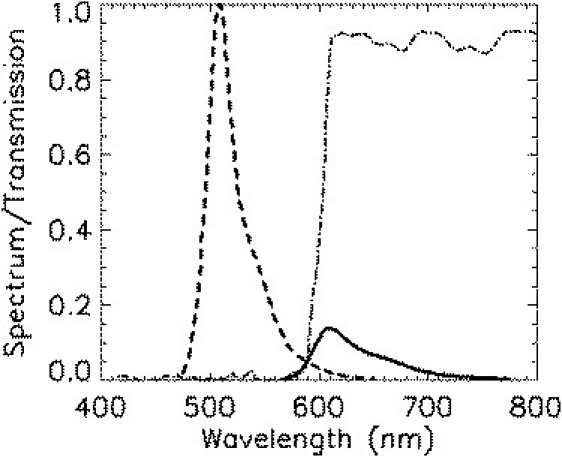
Fluorescence emission spectra of EGFP (dashed curve) and mCherry (solid curve) are plotted together with the transmission curve of the dichroic mirror (dot-dashed curve) used to separate the fluorescence into two channels. The green channel contained an additional 84-nm-wide filter centered at 510 nm to eliminate mCherry fluorescence reflected by the dichroic mirror. The emission spectra are normalized such that their integrated areas are proportional to the brightness.

We use G to denote the short-wavelength channel (“green channel”) and R for the long-wavelength channel (“red channel”). FFS parameters of each channel are distinguished with a subscript label followed by the molecular species. For example, the donor, D, has brightness ${\lambda }_{\mathbf{G},\mathrm{D}}$ in the green channel and brightness ${\lambda }_{\mathbf{R},\mathrm{D}}$ in the red channel, whereas the acceptor has brightness only in the red channel. The brightness of each of the two states is denoted by ${\lambda }_{\mathbf{R},\mathrm{A}\left(1\right)}$ and ${\lambda }_{\mathbf{R},\mathrm{A}\left(2\right)}$.

When D and A interact, FRET might happen. We treat D as the donor and A as the acceptor, which corresponds to the experimentally relevant case where D = EGFP and A = mCherry. Suppose the two proteins interact to form a hetero-oligomer ${\mathrm{D}}_m{\mathrm{A}}_n$. It is of interest to predict the experimental FFS parameters of ${\mathrm{D}}_m{\mathrm{A}}_n$ theoretically. Because the description of FRET is complex, we first consider the heterodimer DA, which is the simplest hetero-oligomer ($m=n=1$).

Brightness of heterodimer DA

A microscopic picture of the heterodimer DA takes the two brightness states of A into account, which leads to the states DA(1) and DA(2) with population fractions of α and $1-\alpha$, respectively. Each microscopic state DA(x) is associated with its own FRET efficiency $E_{\text{DA}\left(x\right)}$$\left(x=1,2\right)$. The relationship between the brightness and the FRET efficiency described previously (8,22) also applies to the microscopic states:

$$\begin{array}{l}{\lambda }_{\mathbf{R},\text{DA}\left(\text{x}\right)}={\lambda }_{\mathbf{R},\mathrm{D}}\left(1-E_{\text{DA}\left(x\right)}\right)+{\lambda }_{\mathbf{R},\mathrm{A}\left(\text{x}\right)}\left(1+E_{\text{DA}\left(x\right)}\frac{{\sigma }_{\mathrm{D}}}{{\sigma }_{\mathrm{A}\left(x\right)}}\right)\text{.}\\ {\lambda }_{\mathbf{G},\text{DA}\left(\text{x}\right)}={\lambda }_{\mathbf{G},\mathrm{D}}\left(1-E_{\text{DA}\left(x\right)}\right)\end{array}$$ (6)

The symbol ${\sigma }_{\text{Y}}$ denotes the two-photon cross section of species Y. Once we know the brightness and fraction of each state, the (i,j)th bivariate factorial cumulant is readily calculated (23) as

$${\kappa }_{[i,j]}={\gamma }_{i+j}N{T}^{i+j}\left(\alpha {\lambda }_{\mathbf{R},\text{DA}\left(1\right)}^i{\lambda }_{\mathbf{G},\text{DA}\left(1\right)}^j+\left(1-\alpha \right){\lambda }_{\mathbf{R},\text{DA}\left(2\right)}^i{\lambda }_{\mathbf{G},\text{DA}\left(2\right)}^j\right)\text{.}$$ (7)

These cumulants provide an exact description of the heterodimer DA accounting for the population mix of DA(1) and DA(2). It is necessary to relate the cumulants to the observable parameters of an FFS experiment, such as brightness, number of molecules, and fluctuation amplitude. Again, a composite description is used, where the mix of microscopic brightness states is approximated by a single state. A tilde is used to denote composite parameters, as done earlier for homo-oligomers. We first consider single-channel analysis, which determines composite parameters for the brightness and autocorrelation amplitude for the red channel,

$${\tilde{\lambda }}_{\mathbf{R},\text{DA}}=\frac{{\kappa }_{[2,0]}}{{\gamma }_{2}T{\kappa }_{[1,0]}},\tilde{G}{\left(0\right)}_{\mathbf{R},\text{DA}}=\frac{{\gamma }_2}{{\tilde{N}}_{\mathbf{R},\text{DA}}}=\frac{{\kappa }_{\left[2,0\right]}}{{\kappa }_{\left[1,0\right]}^2},$$ (8)

and the green-channel,

$${\tilde{\lambda }}_{\mathbf{G},\text{DA}}=\frac{{\kappa }_{[0,2]}}{{\gamma }_{2}T{\kappa }_{[0,1]}},\tilde{G}{\left(0\right)}_{\mathbf{G},\text{DA}}=\frac{{\gamma }_2}{{\tilde{N}}_{\mathbf{G},\text{DA}}}=\frac{{\kappa }_{\left[0,2\right]}}{{\kappa }_{\left[0,1\right]}^2}\text{.}$$ (9)

Note that the numbers of molecules determined in the red and green channel are not identical, ${\tilde{N}}_{\mathbf{G},\text{DA}}\ne {\tilde{N}}_{\mathbf{R},\text{DA}}$, which is a consequence of approximating the heterodimer by a single species. The cumulants also allow us to calculate the cross-correlation amplitude,

$$\tilde{G}{\left(0\right)}_{\mathbf{RG},\text{DA}}=\frac{{\kappa }_{\left[1,1\right]}}{{\kappa }_{\left[0,1\right]}{\kappa }_{\left[1,0\right]}}\text{.}$$ (10)

We will frequently use Eqs. 8–10 to compare the predicted composite parameters with the experimentally determined FFS values. The simple analytical nature of these equations provides a convenient method for checking the validity of the proposed two-state model of mCherry.

Another, more powerful approach is to simultaneously fit all cumulants to a model, as previously described (23), which we refer to as dual-color analysis. We later measure a heterodimer and fit its cumulants with a two-species model to find the properties of states DA(1) and DA(2). The two-species fit directly determines the microscopic brightness values (${\lambda }_{\mathbf{R},\text{DA}\left(1\right)}$, ${\lambda }_{\mathbf{G},\text{DA}\left(1\right)}$, ${\lambda }_{\mathbf{R},\text{DA}\left(2\right)}$, ${\lambda }_{\mathbf{G},\text{DA}\left(2\right)}$), which, with the help of Eq. 6, serve to identify the missing parameters of the two-state model.

We also introduce a dual-color composite description of the heterodimer, where the mix of microscopic brightness states is approximated by a single state. The fit of the cumulants to a single species determines the composite brightness in each channel (${\tilde{\Lambda }}_{\mathbf{G},\text{DA}}$, ${\tilde{\Lambda }}_{\mathbf{R},\text{DA}}$). We use different symbols to distinguish the composite parameters of the dual-channel (or dual-color) analysis from the parameters of the single-channel analysis (Eqs. 8 and 9), because these methods yield different composite brightness values, ${\tilde{\Lambda }}_{\mathbf{R},\text{DA}}\ne {\tilde{\lambda }}_{\mathbf{R},\text{DA}}$. This deviation reflects different ways of approximating the two states of the heterodimer. A disadvantage of dual-color analysis over single-channel analysis is that no analytical solution exists, and a fit is required to determine the composite parameters. However, dual-color analysis contains more information than single-channel analysis and is used later to resolve a mixture of fluorescent proteins.

The brightness of the microscopic state DA(x) depends on its FRET efficiencies,$E_{\text{DA}\left(x\right)}$, which are usually difficult to determine experimentally. In contrast, the average FRET efficiency is readily determined by experiment. Therefore, it is useful to relate the microscopic FRET efficiencies to the average FRET efficiency $\langle E\rangle$. We get the following relation from the definition of the average FRET efficiency,

$$\langle E\rangle =1-\frac{\alpha {\left(1-E_{\text{DA}\left(1\right)}\right)}^2+(1-\alpha ){\left(1-E_{\text{DA}\left(2\right)}\right)}^2}{\alpha \left(1-E_{\text{DA}\left(1\right)}\right)+(1-\alpha )\left(1-E_{\text{DA}\left(2\right)}\right)}\text{.}$$ (11)

Next, we introduce the ratio between the FRET transfer rates of both states, $\xi =k_{\text{DA}\left(2\right)}^T/k_{\text{DA}\left(1\right)}^T$, which provides another relation between the FRET efficiencies,

$$E_{\text{DA}\left(2\right)}=\frac{E_{\text{DA}\left(1\right)}\xi }{1+\left(\xi -1\right)E_{\text{DA}\left(1\right)}}\text{.}$$ (12)

We assume that the transfer rate ratio, ξ, between two microscopic states is approximately constant, independent of the average FRET efficiency. The transfer rate depends on the absorption cross section of the acceptor and the angle between the donor emission and the acceptor absorption dipole. Since the cross section, ${\sigma }_{\mathrm{A}\left(i\right)}$, does not change, assuming a constant ξ implies that the angle between donor and acceptor is isotropically averaged, which provides a reasonable starting point in the absence of additional structural information. The parameter ξ is determined later by experiment.

Combining Eqs. 11 and 12, the FRET efficiency of state DA(x) can be expressed as a function of ξ, $\langle E\rangle$, and α,

$$E_{\text{DA}\left(x\right)}=f_x\left(\langle E\rangle ,\xi ,\alpha \right)\text{.}$$ (13)

Once ξ and α are known, $E_{\text{DA}\left(x\right)}$ is calculated from the average FRET efficiency. The average FRET efficiency is experimentally obtained by a fluorescence lifetime measurement of the donor. An alternative way of determining its value is to compare the green-channel brightness of the sample, ${\tilde{\lambda }}_{\mathbf{G},\text{DA}}$, to the intrinsic brightness of the donor, ${\lambda }_{\mathbf{G},\text{D}}$:

$$\langle E\rangle =1-\frac{{\tilde{\lambda }}_{\mathbf{G},\text{DA}}}{{\lambda }_{\mathbf{G},\mathrm{D}}}\text{.}$$ (14)

The validity of Eq. 14 is easily shown by inserting the definition of the brightness into the equation. We noticed that lifetime and brightness measurements determine slightly different FRET efficiencies. The deviation between the two methods is larger than experimental uncertainty, but its origin is currently unknown. We use brightness to determine FRET efficiency in this article. This approach has the advantage that a fluorescence lifetime setup is not required, because all parameters are determined by the FFS measurement.

Brightness of hetero-oligomer DA_n

A higher-order hetero-oligomer contains multiple acceptors. Because the description of all microscopic states is complex, we restrict ourselves to the case of a single donor with multiple acceptors. We use the heterotrimer DA₂ as an example to illustrate the modeling approach. There are four microscopic states DA₁(1)A₂(1), DA₁(1)A₂(2), DA₁(2)A₂(1), and DA₁(2)A₂(2), with individual acceptors identified by a subscript. Because the distance from the donor to acceptors A₁ and A₂ will generally not be the same, the FRET efficiency of each acceptor is different and explicitly depends on the microscopic states of the other acceptor. If the FRET efficiencies are known, it is straightforward to calculate the cumulants and the brightness of the heterotrimer. However, in most cases, the individual FRET efficiencies are unknown and an approximation is needed to evaluate FFS parameters. A detailed treatment of the two-state mCherry model applied to a hetero-oligomer DA_n is described in Appendix A.

Materials and Methods

FFS

The dual-channel two-photon fluorescence fluctuation instrumentation has been described previously (23). All experiments are performed with an excitation wavelength of 1000 nm. The fluorescence emission is separated into two different detection channels with a 580-nm dichroic mirror (Chroma Technology, Rockingham, VT). The green channel is equipped with an 84-nm-wide bandpass filter centered at 510 nm (Semrock, Rochester, NY) to eliminate the reflected fluorescence of mCherry. All cellular measurements are conducted with a sampling frequency of 20 kHz, and the data acquisition time is 1 min for most experiments. The single-channel brightness is obtained with $Q\left(\tau \right)$ analysis (24). All experimental correlation curves are fit to the simple diffusion model,

$$G\left(t\right)=G\left(0\right){\left(1+\frac{t}{{\tau }_{\mathrm{d}}}\right)}^{-1}{\left(1+\frac{t}{{\tau }_{\mathrm{d}}r}\right)}^{-\frac{1}{2}}\text{.}$$ (15)

where ${\tau }_{\mathrm{d}}$ is the diffusion time and r is calibrated from a measurement of a dye solution. The correlation amplitude is inversely proportional to the number of molecules $G\left(0\right)={\gamma }_2/N$, where ${\gamma }_2=1/\left(2\sqrt{2}\right)$ is used throughout this article (19).

The laser power at the sample is ∼1 mW. No saturation of EGFP or mCherry occurs at these conditions, since brightness varies quadratically as the excitation power is doubled. Typical data acquisition times in cells range from 30 to 120 s. No loss of fluorescence intensity is detected for the data acquisition times used.

Single-color and dual-color time-integrated fluorescence cumulant analysis (TIFCA) is performed as previously described (19,23). The raw photon counts are rebinned to obtain cumulants for different sampling times. The univariate (single-color) and bivariate (dual-color) factorial cumulants of the photon counts are fit to models assuming a single or two brightness states. The quality of the fit is judged by the reduced χ². The fit determines brightness, diffusion time, and the number of fluorescent molecules in the observation volume of each species.

Lifetime

The instrumentation and data analysis for lifetime measurements has been described in Hillesheim et al. (8). Briefly, a TCSPC card (TimeHarp 200, Picoquant, Berlin, Germany) receives the synchronization signal from a photodiode (DET210, Thorlabs, Newton, NJ) that registers the 80-MHz pulse train of the laser. The photon counts are recorded under magic angle conditions with a photomultiplier tube (H7421-40, Hamamatsu, Bridgewater, NJ). The instrument response function is determined via second harmonic generation on urea crystals (ICN Biomedical, Aurora, OH). Solutions of sulforhodamine 101 in aqueous solution and in 60%/40% glycerol/water are used as controls. The fluorescence intensity decay of fluorescent proteins is measured in the nucleus of CV-1 cells under the same experimental condition used for FFS experiments. A 525/50 nm bandpass filter (Semrock) is placed before the PMT to select only the fluorescence of EGFP and EYFP. The lifetime data were analyzed using Globals Unlimited (Urbana, IL) and software written in Interactive Data Language (ITT Visual Information Solutions, Boulder, CO).

Sample preparation and plasmid construction

The mCherry pRSET B plasmid was a kind gift from Dr. R. Y. Tsien (University of California, San Diego). mCherry was amplified by polymerase chain reaction (PCR) with a $5\prime$ primer that encodes an NheI restriction site and a $3\prime$ primer that encodes an XhoI site. The PCR fragment of mCherry was ligated into the backbone of pEGFP-C1 (Clonetech, Mountainview, CA) to generate the mCherry-C1 vector for mammalian expression. For the sake of brevity we refer to EGFP as G, to EYFP as Y, and to mCherry as Ch when naming protein constructs. The fusion proteins Ch-Ch and Ch-G were constructed by inserting PCR-amplified mCherry or EGFP into the mCherry-C1 vector at SacII and BamHI sites. G-Ch (Y-Ch) was constructed by inserting mCherry into the pEGFP-C1 (pEYFP-C1) vector at SacII and BamHI sites. The ligand binding domains of retinoid X receptor (RXRLBD) and retinoic acid receptor (RARLBD) from mouse ($\text{mRXR}\beta$ and $\text{mRAR}\alpha$) were inserted into the mCherry-C1 plasmid at the XhoI and EcoRI sites to construct Ch-RARLBD and Ch-RXRLBD. G-Ch and Ch-Ch were further digested at XhoI and EcoRI sites, and either an EGFP or RARLBD PCR fragment was ligated into the vectors to generate G-RARLBD-Ch, Ch-G-Ch, and Ch-RARLBD-Ch constructs. The Supporting Material (Linker of mCherry-EGFP fusion constructs) contains information about the linker sequences that connect the fusion proteins. The Ch-RXRLBD experiments are performed in the presence of the RXR-specific ligand 9-cis retinoic acid at a concentration of 1 μM.

CV-1 cells were obtained from American Type Culture Collection (Manassas, VA) and maintained in 10% fetal bovine serum (Invitrogen, Carlsbad, CA) and Dulbecco's modified Eagle's medium (Biowhittaker, Walkersville, MD). Cells were subcultured into eight-well coverglass chamber slides (Nalge-Nunc International, Rochester, NY) and then transiently transfected using transfectin (Bio-Rad, Hercules, CA) according to the manufacturer's instructions. Before conducting measurements, the growth media was removed and replaced with Leibovitz L15 (Invitrogen, Carlsbad, CA). All measurements were performed in the cell nucleus.

Results and Discussion

Monomer and dimer of mCherry

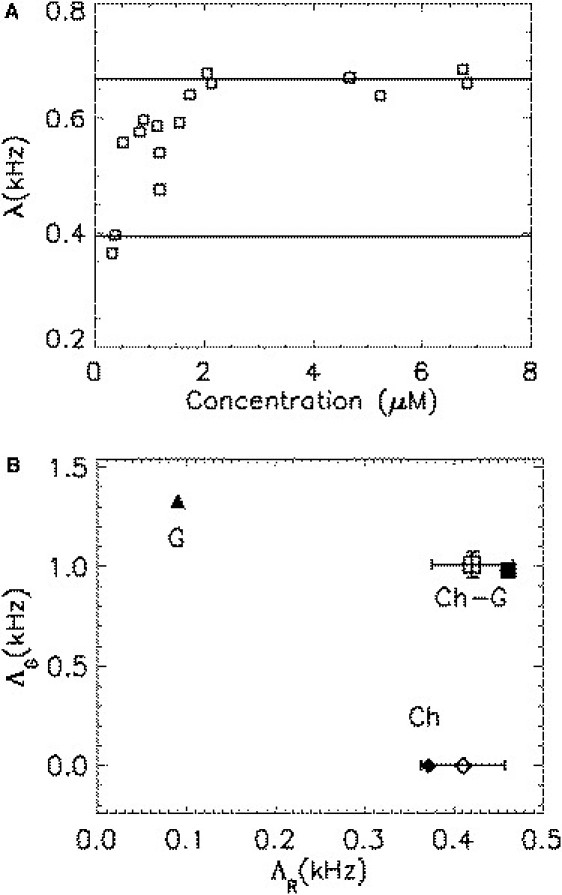
CV-1 cells are transiently transfected with mCherry as described in Materials and Methods. The laser is focused into the nucleus of the cell and data are acquired for 1 min. In Fig. 2 A, the brightness of mCherry (triangles) is plotted as a function of concentration. We notice a constant brightness of ∼390 cps over the concentration range studied. This observation shows that mCherry remains a monomeric protein up to at least 25 μM (the concentration has been corrected for bias with Eq. 5. Because mCherry is not very bright, the presence of two brightness states is not yet discernible and the FFS experiment determines the composite brightness ${\tilde{\lambda }}_{\mathbf{R},\mathrm{A}}$ of the mCherry monomer. We also measure the brightness of a fusion protein of mCherry with the ligand-binding domain of the nuclear receptor RAR (denoted as Ch-RARLBD) as a function of protein concentration (Fig. 2 A, squares). Because RARLBD is known to be monomeric (15,22), we expect that the brightness of the fusion protein matches that of mCherry, as confirmed by the data. This result also demonstrates that mCherry retains its fluorescence brightness value in a fusion construct.

Figure 2.

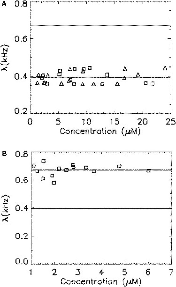
Brightness of monomeric and homodimeric mCherry is plotted as a function of protein concentration. Each symbol represents a measurement for a different cell. The concentration has been corrected for the bias due to the two states of mCherry (Eq. 5). (A) The brightness of mCherry (triangles) is concentration-independent, as expected for a monomeric protein. The brightness of mCherry-RARLBD (squares) equals that of mCherry, indicating that labeling does not change the brightness of mCherry. (B) The brightness of the homodimer Ch-RARLBD-Ch (squares) is concentration-independent, but less than twice the brightness of monomeric mCherry.

If mCherry exists in a single brightness state, the brightness of the dimer is expected to be twice that of the monomer, as has been confirmed for the proteins EGFP (15) and EYFP (see Table S1 of the Supporting Material). To test this hypothesis, we construct the homodimer Ch-RARLBD-Ch, where the two mCherries are separated by the protein RARLBD. The reason for this particular choice of fusion protein will be addressed at a later point. The brightness of Ch-RARLBD-Ch is concentration-independent (Fig. 2 B), as expected. However, the brightness of the dimer is less than twice the monomer brightness. The data of Fig. 2 lead to a brightness ratio $b_{{\mathrm{A}}_2}={\tilde{\lambda }}_{\mathbf{R},{\mathrm{A}}_2}/{\tilde{\lambda }}_{\mathbf{R},\mathrm{A}}$ of $1.7\pm 0.05$. This result establishes that mCherry is not described by a single brightness state. The ratio of the dimer/monomer brightness $b_{{\mathrm{A}}_2}$ is a crucial parameter needed to predict the brightness of the oligomer A_n. It is also needed to determine the molecular fraction α and brightness ratio θ of the mCherry states (Eq. 4).

Microscopic states of mCherry

A fusion protein of EGFP and mCherry (G-Ch) is used to demonstrate that mCherry exists in two microscopic states and to determine at the same time its parameters. We first perform fluorescence lifetime experiments on EGFP and G-Ch. The time-resolved fluorescence decay, $F\left(t\right)$, of EGFP by itself is well described by a single-exponential process with a lifetime of ${\tau }_{\mathrm{d}}=2.58\pm 0.04\text{ns}$ (n = 17 cells) (see Fig. S1A). The results of the lifetime measurements are presented in more detail in the Supporting Material, together with a discussion of other measurements reported in the literature. In contrast to EGFP alone, its fluorescence lifetime in the fusion protein G-Ch requires a double exponential model to describe the data (see Fig. S2). If mCherry exists in a single state, we expect a monoexponential decay of the donor EGFP, with a shortened lifetime that characterizes the FRET transfer efficiency. The presence of a double-exponential decay is consistent with the presence of two microscopic states of mCherry. In the Theory section, the heterodimer DA (with D = EGFP and A = mCherry) is described as a mixture of DA(1) with molecular populationα and DA(2) with molecular population $1-\alpha$. In general, the fluorescence transfer rates from the donor to these two acceptor states will be different, which leads to a biexponential decay of the donor fluorescence,

$$F\left(t\right)=C_1\text{exp}\left(-t/{\tau }_1\right)+C_2\text{exp}\left(-t/{\tau }_2\right),$$ (16)

A fit of the fluorescence intensity decay to Eq. 16 determines the ratio between preexponential amplitudes, $C_1/C_2=0.3\pm 0.04$, and the two lifetimes (${\tau }_1=0.84\pm 0.12\text{ns}$, ${\tau }_2=2.42\pm 0.04\text{ns}$). Because EGFP exists in a single state, the preexponential amplitude is directly proportional to the molecular population. The fit determined molecular populations of $\alpha =0.23\pm 0.03$ and $(1-\alpha )=0.77\pm 0.03$ for the two states. Inserting the population fraction $\alpha =0.23$ and the brightness ratio $b_{{\mathrm{A}}_2}=1.7$ into Eq. 3 determines the brightness ratio between the two mCherry states, $\theta ={\lambda }_{\mathrm{A}\left(2\right)}/{\lambda }_{\mathrm{A}\left(1\right)}=0.29$. These parameters relate the microscopic brightness to the composite brightness via Eq. 2: ${\lambda }_{\mathbf{R},\mathrm{A}\left(1\right)}=1.54{\tilde{\lambda }}_{\mathbf{R},\mathrm{A}}$ and ${\lambda }_{\mathbf{R},\mathrm{A}\left(2\right)}=0.45{\tilde{\lambda }}_{\mathbf{R},\mathrm{A}}$.

We next perform a dual-channel FFS experiment on EGFP and mCherry. Dual-color time-integrated fluorescence cumulant analysis (TIFCA) (23) determines the brightness of the EGFP and mCherry in each channel, ${\lambda }_{\mathbf{G},\mathrm{D}}=1260\pm 70\text{cps}$, ${\lambda }_{\mathbf{R},\mathrm{D}}=90\pm 30\text{cps}$, and ${\tilde{\lambda }}_{\mathbf{R},\mathrm{A}}=360\pm 40\text{cps}$. The brightness of each microscopic state of mCherry is calculated as ${\lambda }_{\mathbf{R},\mathrm{A}\left(1\right)}=1.54{\tilde{\lambda }}_{\mathbf{R},\mathrm{A}}=560\text{cps}$ and ${\lambda }_{\mathbf{R},\mathrm{A}\left(2\right)}=0.45{\tilde{\lambda }}_{\mathbf{R},\mathrm{A}}=160\text{cps}$. To determine the remaining parameters of the microscopic mCherry states, the heterodimer Ch-G is measured by FFS. Because the heterodimer sample contains a mixture of two microscopic states, DA(1) and DA (2), the FFS data are fit by dual-color TIFCA to a two-species model to determine the microscopic brightnesses of the two states. The only constraint applied to the fit specifies that the population fraction of the first state equals $\alpha =0.23$. The brightness of state 1 is determined as ${\lambda }_{\mathbf{R},\text{DA}\left(1\right)}=850\pm 60\text{cps}$ and ${\lambda }_{\mathbf{G},\text{DA}\left(1\right)}=320\pm 60\text{cps}$, whereas the brightness of state 2 is ${\lambda }_{\mathbf{R},\text{DA}\left(2\right)}=370\pm 30\text{cps}$ and ${\lambda }_{\mathbf{G},\text{DA}\left(2\right)}=980\pm 80\text{cps}$. By comparing the experimental brightness values using Eq. 6, we determine the FRET efficiencies ($E_{\text{DA}\left(1\right)}=0.75\pm 0.06$ and $E_{\text{DA}\left(2\right)}=0.22\pm 0.05$) and the two-photon cross-section ratios (${\sigma }_{\mathrm{D}}/{\sigma }_{\mathrm{A}\left(1\right)}=0.66\pm 0.1$ and ${\sigma }_{\mathrm{D}}/{\sigma }_{\mathrm{A}\left(2\right)}=3.9\pm 1.2$). The two FRET efficiencies lead to a ratio of the transfer rate coefficients of $\xi =0.096\pm 0.023$ according to Eq. 12. Now, all parameters describing the two states of mCherry are known. We have repeated the experiments several times to determine an optimized parameter set, which is given in Table 1 and used throughout this article.

Table 1.

Photophysical properties of the two states of mCherry

State i	${\alpha }_{\text{Ch}\left(i\right)}$	${\lambda }_{\text{Ch}\left(i\right)}/{\tilde{\lambda }}_{\text{Ch}}$	${\sigma }_{\text{EGFP}}/{\sigma }_{\text{Ch}\left(i\right)}$	$k_{\text{Ch}\left(i\right)}^T/k_{\text{Ch}\left(2\right)}^T$
1	0.23	1.54	0.66	10
2	0.77	0.45	4.24	1

Meanings of symbols and the derivation of values are explained in the text.

Test of the two-state model

To build confidence in this parameter set, we perform additional experiments to check their consistency with the two-state model.

Earlier fluorescence lifetime measurements of the donor of the G-Ch fusion protein revealed two lifetime components with a population fraction of $\alpha =0.23$ for the first state, which we attributed to the difference in FRET efficiency to each acceptor state of mCherry. We now perform the same experiment on a fusion protein of EYFP and mCherry (Y-Ch). If mCherry exists in two states, we expect to recover the same molecular fractions from the lifetime data of Y-Ch as from that of the G-Ch fusion protein. EYFP is also described by a single-exponential model with a longer lifetime (${\tau }_{\mathrm{D}}=3.07\text{ns}$) than EGFP (see Fig. S1B) and a red-shifted emission spectrum. The fluorescence decay of the donor EYFP in Y-Ch requires a double-exponential fit (Eq. 16), which recover two lifetimes (${\tau }_1=0.75\pm 0.11\text{ns}\text{and}{\tau }_2=2.73\pm 0.07\text{ns}$) (see Fig. S3) and the population fraction of state 1, $\alpha =0.24\pm 0.03$, which is identical to that obtained for G-Ch.

The time-resolved fluorescence decay $F\left(t\right)$ of mCherry is not described by a single-exponential process (9). We fit the fluorescence decay of mCherry to a biexponential model (Eq 16), which describes the experimental data within error (${\tau }_1=0.90\pm 0.08$ns, ${\tau }_2=1.94\pm 0.07$ns, and $C_2/C_1=0.64\pm 0.09$). The preexponential ratio is converted into a population fraction, α, as detailed in Appendix A. Equations 3 and 23 determine the value of α and θ. Since Eq. 3 is quadratic, two solutions are obtained. The first solution ($\alpha =0.18$ and $\theta =0.29$) closely matches the parameters obtained earlier (Table 1).

We also perform a dual-color FFS experiment on the G-Ch fusion protein and fit the data to a two-species model with the constraint $\alpha =0.23$ to determine the microscopic brightness values of DA(1) and DA(2). The brightness values of the fit (${\lambda }_{\mathbf{R},\text{DA}\left(1\right)}=810\pm 70\text{cps}$, ${\lambda }_{\mathbf{G},\text{DA}\left(1\right)}=540\pm 60\text{cps}$, ${\lambda }_{\mathbf{R},\text{DA}\left(2\right)}=350\pm 30\text{cps}$, and ${\lambda }_{\mathbf{G},\text{DA}\left(2\right)}=1070\pm 80\text{cps}$) determine the two-photon cross-section ratios (${\sigma }_{\mathrm{D}}/{\sigma }_{\mathrm{A}\left(1\right)}=0.67\pm 0.1$ and ${\sigma }_{\mathrm{D}}/{\sigma }_{\mathrm{A}\left(2\right)}=4.6\pm 1.4$) and the FRET efficiencies ($E_{\text{DA}\left(1\right)}=0.58\pm 0.05$ and $E_{\text{DA}\left(2\right)}=0.15\pm 0.06$), which correspond to a ratio of $\xi =0.13\pm 0.05$ for the transfer rate coefficients.

Every experiment described in this section supports the two-state model of mCherry, and the parameters agree within experimental error with the values compiled in Table 1. In the next two sections, we examine the consequences of the two-state model of mCherry for FCS and brightness analysis.

Single-channel and cross-correlation FCS of heterodimers

We measure the single-channel brightness and correlation amplitudes of different heterodimers and compare the experimental results with the model predictions based on Eqs. 8–10. The experiments are conducted on G-Ch and Ch-G. In addition, we construct a fusion protein of EGFP and mCherry separated by the ligand-binding domain of retinoic acid receptor (RARLBD). The triple construct, G-RARLBD-Ch serves as a model of a heterodimer with a small FRET efficiency.

The analysis of the data proceeds as follows. First, we determine the average FRET efficiency, $\langle E\rangle$, of each sample from the brightness in the green channel, ${\tilde{\lambda }}_{\mathbf{G},\text{DA}}$, by comparing it to the intrinsic brightness of the donor, ${\lambda }_{\mathbf{G},\mathrm{D}}$, according to Eq. 14. Next, we calculate the cumulants using the model parameters of Table 1 and the FRET efficiency of each state, $E_{\text{DA}\left(x\right)}=f_x\left(\langle E\rangle ,\xi ,\alpha \right)$. Equation 8 allows us to predict the brightness in the red-channel, ${\tilde{\lambda }}_{\mathbf{R},\text{DA}}$, for each of the three heterodimers. The effect of the average FRET efficiency on the red-channel brightness, ${\tilde{\lambda }}_{\mathbf{R},\text{DA}}$, of a heterodimer is shown in Fig. 3 A together with the experimentally measured values. A comparison of the measured and predicted brightness values shows excellent agreement between experiment and model.

Figure 3.

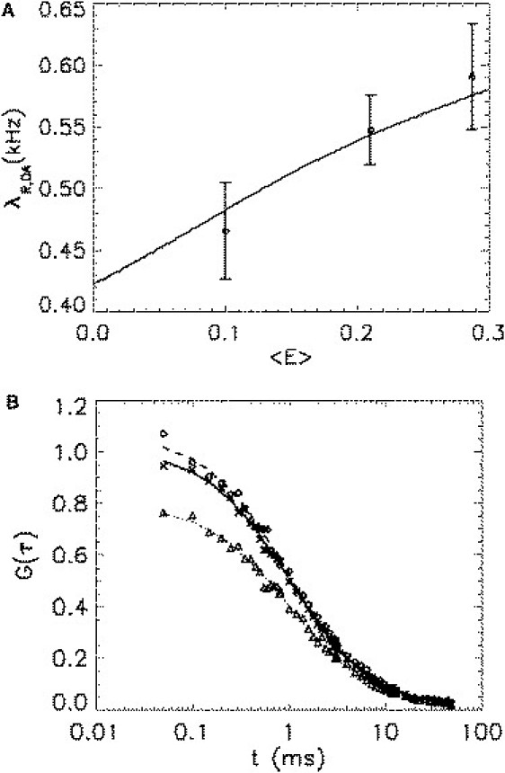
Single-channel and cross-correlation analysis of hetero-dimers. (A) The solid line shows the red-channel brightness of a heterodimer DA as a function of the average FRET efficiency as predicted by the two-state model with parameters taken from Table 1. The symbols represent the experimentally determined red-channel brightness and average FRET efficiency of three heterodimers (G-RARLBD-Ch, G-Ch, and Ch-G). (B) The red-channel autocorrelation function (diamonds) and the cross-correlation function (triangles) of Ch-G are compared with the green-channel autocorrelation function (exes). The experimental correlation curves are normalized with respect to the green-channel autocorrelation amplitude and then averaged across 10 cells. The lines represent the fit of the data to a simple diffusion model (Eq. 15). The three correlation curves do not overlap as a result of the two-state model of mCherry. The difference in the correlation amplitudes agrees with the two-state model as shown in Table 2.

The auto- and cross-correlation functions of a single fluorescent species are identical if the fluorophore exists in a single brightness state and the optics of the instrument is properly aligned. We experimentally confirmed the identity of the correlation functions for the dye rhodamine 6G as a control (data not shown). However, the measured auto- and cross-correlation functions of each heterodimer have different amplitudes (Table 2). This difference is a consequence of mCherry existing in two states. The two-state model of mCherry predicts that the heterodimer sample is a mixture of states DA(1) and DA(2), which leads to nonoverlapping correlation functions. The auto- and cross-correlation functions of Ch-G with amplitudes normalized to that of the green channel are shown in Fig. 3 B to illustrate the mismatch. The figure reveals that the red-channel G(0) is larger than the green-channel G(0) as a result of the additional fluctuation introduced by the two states of mCherry. The ratio between the correlation amplitudes $\tilde{G}{\left(0\right)}_{\mathbf{R},\text{DA}}/\tilde{G}{\left(0\right)}_{\mathbf{G},\text{DA}}$ and $\tilde{G}{\left(0\right)}_{\mathbf{RG},\text{DA}}/\tilde{G}{\left(0\right)}_{\mathbf{G},\text{DA}}$ is determined from a fit of the experimental correlation curves to Eq. 15. Table 2 compares the experimental ratios to the ones predicted by the two-state model. The experimental result is in good agreement with the theoretical prediction.

Table 2.

Correlation amplitude ratios

	$\tilde{G}{\left(0\right)}_{\mathrm{R}}/\tilde{G}{\left(0\right)}_{\mathrm{G}}$		$\tilde{G}{\left(0\right)}_{\text{RG}}/\tilde{G}{\left(0\right)}_{\mathrm{G}}$
	Experiment	Theory	Experiment	Theory
G-RARLBD-Ch	1.12 ± 0.06	1.21	0.91 ± 0.05	0.90
G-Ch	1.12 ± 0.08	1.11	0.85 ± 0.04	0.81
Ch-G	1.05 ± 0.1	1.03	0.78 ± 0.06	0.78
Ch-G-Ch	0.85 ± 0.05	0.90	0.69 ± 0.06	0.73

Auto- and cross-correlation functions of hetero-oligomer involving mCherry do not overlap, because mCherry exists in two states. The correlation amplitudes G(0) are normalized with respect to the green channel G(0). The experimental values and uncertainties are obtained by averaging over measurement of 10 cells. The two-state model predicts the correlation amplitude according to Eqs. 8–10, and the results show excellent agreement with the experimental values.

Higher-order hetero-oligomer DA_n

We now consider the case of multiple acceptors. As pointed out in the Theory section, it is generally impossible to determine each individual FRET efficiency, $E_{{\text{DA}}_{\text{j}}\left(x\right)}$. Thus, an approximation is needed, if we want to use the microscopic model. We now explicitly describe the experimental approach for the case of a heterotrimer DA₂. Generalization to the case DA_n is straightforward. Each of the two acceptors of DA₂ has a different probability of receiving the transferred energy. Thus, each acceptor receives, on average, a certain fraction of the transferred energy. The partition of the transferred energy depends on the structure of the heterotrimer and affects its brightness. However, as pointed out in Appendix A, two limiting cases exist: 1), all acceptors are equivalent and receive an equal share of the FRET energy; and 2), all energy is transferred to a single acceptor only. The brightness for all other cases lies between the brightness values obtained for the two limiting cases. Knowledge of the average FRET efficiency is sufficient to calculate the FFS parameters of the two limiting cases. Fig. 4 A shows the red-channel brightness, ${\tilde{\lambda }}_{\mathbf{R},{\text{DA}}_2}$, of the two limiting cases as a function of the average FRET efficiency. The relative deviation between both limiting cases is <3%, which is smaller than the typical experimental uncertainty. Because the exact brightness of a general heterotrimer DA₂ lies between both curves, we are allowed to use any of the two extreme cases as an approximation. We choose the case where all acceptors are equivalent as our approximate model for calculating the two-state model. The above analysis shows that the deviation introduced by the approximation is, from an experimental point of view, negligible for the heterotrimer. By repeating the same analysis, it is possible to show that the same approximation works well for modeling higher-order oligomers.

Figure 4.

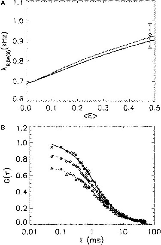
Brightness and correlation amplitudes of the heterotrimer DA₂. (A) The red-channel brightness of the heterotrimer DA₂ is shown as a function of the average FRET efficiency for two limiting cases, one where both mCherries are equivalent (solid line), and one where all energy is transferred to a single mCherry (dotted line). The deviation between the two extreme cases is smaller than the typical experimental uncertainty. The red-channel brightness of the fusion protein Ch-G-Ch (diamonds) agrees, within experimental error, with either limiting case. (B) The red-channel (diamonds), green-channel (exes), and cross-channel (triangles) correlation curves of Ch-G-Ch are analyzed as described in the legend for Fig. 3B. Note that the correlation amplitude of the red channel is lower than that of the green channel, as theoretically predicted by the two-state model. The cross-correlation amplitude is also correctly predicted by the model as summarized in Table 2.

We now measure the triple fusion protein mCherry-EGFP-mCherry (Ch-G-Ch) and compare the experimental values with the two-state model. The data are analyzed assuming that each acceptor receives equal amount of energy from the donor, as discussed above. The measured brightness in the green channel is used to calculate the average FRET efficiency, $\langle E\rangle =0.48$. We next calculate the red-channel brightness and compare the result with the experimental value (Fig. 4 A). Model and experiment are in good agreement.

The auto-/cross-correlation curves of Ch-G-Ch are graphed in Fig. 4 B. We observe with interest that the red-channel autocorrelation amplitude is less than that of the green channel: $\tilde{G}{\left(0\right)}_{\mathbf{R},{\text{DA}}_2}/\tilde{G}{\left(0\right)}_{\mathbf{G},{\text{DA}}_2}=0.85\pm 0.05$. The experimental ratios of the correlation amplitudes are shown, together with the values predicted by the two-state model, in Table 2. The model accurately predicts the experimental results.

Interconversion of brightness states of mCherry?

We established the presence of two states for mCherry and implicitly treated each state as static in our models. For this picture to be correct, either the states are not able to interconvert, or they interconvert on a timescale much slower than the diffusion time of mCherry, so that the probability that state A(i) switches while passing the observation volume is negligible. However, we have not yet examined this assumption experimentally. Because the two states differ in their brightness, the correlation function of FFS is able to identify interconversion between the two states as a blinking process (25,26). To address this question, we conducted FCS experiments on purified mCherry in solution. To eliminate the artifacts in the detecting process, we used a 50/50 beam splitter to divide the fluorescence into two channels and study the cross-correlation curves. To explore different timescales, we used glycerol to increase the diffusion time.

Fig. 5 A displays the normalized experimental cross-correlation curve (symbols) of mCherry dissolved in phosphate-buffered saline (PBS). A simple single-species diffusion model (Eq. 15) is sufficient to fit the data (solid line), which returns a diffusion time of 0.23 ms. To explore a longer timescale, we dissolved mCherry in a buffer containing 50% PBS and 50% glycerol by volume. The cross-correlation curve is plotted in Fig. 5 B, which again shows no sign of interconversion. A simple diffusion model fits the data (solid line) and recovers a diffusion time of 1.6 ms. The FCS experiments have been repeated with various excitation laser powers. We obtained a power-independent diffusion time as long as the excitation power was kept low enough that there were no saturation and photobleaching effects (27). We confirmed that the diffusion time for mCherry is, within experimental error, identical to that of the EGFP.

Figure 5.

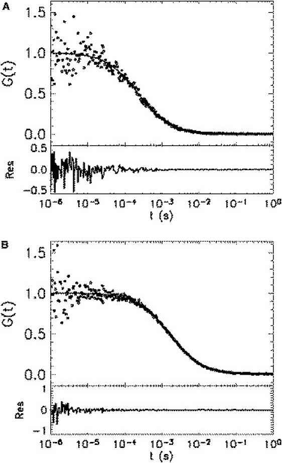
Cross-correlation function of mCherry in solution. (A) Purified mCherry is dissolved in PBS and measured for 10 min with a 50/50 beam splitter. The normalized Experimental cross-correlation function (symbols) is plotted together with the fit (solid line) to Eq. 15. The diffusion time returned from the fit is 0.23 ms, which closely matches that of EGFP measured under the same experimental conditions. (B) Cross-correlation function (symbols) of mCherry in a solution with higher viscosity (PBS with 50% glycerol). A fit (solid line) of the cross-correlation curve to Eq. 15 yields a diffusion time of 1.6 ms. Note that both correlation curves are well described by a simple diffusion model without any additional kinetic processes.

The above experiment demonstrates that the two states are not interconverting on timescales from microseconds to milliseconds for two-photon excitation. We are also able to rule out submicrosecond interconversion, because if the two states interconvert very fast, the molecule can be viewed as a single species with a time-averaged brightness, which would result in a doubling of the brightness for the homodimer of mCherry. These results confirm that treating the mCherry states as static is appropriate for FFS experiments with diffusion times on the millisecond timescale or faster. Our experiments do not provide information about potential interconversion on timescales much longer than milliseconds. Thus, FFS experiments with very slow diffusion (as encountered on membrane systems) need to examine this possibility.

FRET between brightness states of mCherries

FRET between identical fluorophores is termed homo-FRET. If the fluorophore exists in a single state, homo-FRET is not changing the brightness of an oligomeric complex, as seen from Eq. 6, with ${\lambda }_{\mathrm{D}}={\lambda }_{\mathrm{A}}$ and ${\sigma }_{\mathrm{D}}={\sigma }_{\mathrm{A}}$, since donor and acceptor are indistinguishable In addition, the lifetime of the homo-oligomer is identical to that of the monomer. Homo-FRET leads to depolarization of the fluorescence, which in principle could influence brightness. However, such an effect has not been observed (15). We also included data in the supplement that demonstrate that the brightness of dimeric EYFP behaves as expected. If the fluorophore A exists in two distinct states, A(1) and A(2), FRET becomes more complicated. For example, in the case of a homodimer A₂ only the microscopic states A(1)A(1) and A(2)A(2) truly represent pure spectroscopic homodimers, whereas the state A(1)A(2) is, from a spectroscopic point of view, a heterodimer. Thus, homo-FRET of states A(1)A(1) and A(2)A(2) is not affecting their brightness. In contrast, the brightness of A(1)A(2) depends on the amount of FRET in this pair. To clarify the notation, we refer to FRET between different states of a fluorophore as hetero-FRET, which is conceptually identical to hetero-FRET between two distinct fluorescent species.

To ascertain whether hetero-FRET occurs between the two states of mCherry, we measured the lifetime of the heterodimers Ch-Ch and Ch-RARLBD-Ch. Since the two mCherries in Ch-RARLBD-Ch are separated by a large distance, we expect that hetero-FRET does not play a significant role. This expectation is confirmed by experiment, because the fluorescence decay of Ch-RARLBD-Ch is, within experimental uncertainty, identical to that of the mCherry. On the other hand, the two mCherries in Ch-Ch are in close proximity, which should reveal the presence of hetero-FRET. Indeed, we observe that the long-lifetime component is decreased from $1.9\text{ns}$ to $1.65\text{ns}$, whereas the shorter lifetime component is unchanged within experimental error. This experiment further supports the two-state model of mCherry and is consistent with the presence of hetero-FRET between different mCherry states.

Our brightness model of the homocomplex A_n ignored the possibility of hetero-FRET between mCherry states. The reason for this omission is that, experimentally, the influence of hetero-FRET on brightness is quite small for the case of mCherry. Let us consider the homodimer Ch-Ch as an example. In this case, hetero-FRET is only experienced by the pair Ch(1)Ch(2), which comprises only 30% of the total population. Furthermore, if the donor brightness is quenched, the acceptor brightness is enhanced, which moderates the total change in brightness. This argument is supported by the experimentally determined brightness of Ch-Ch, which, compared to that of Ch-RARLBD-Ch, shows a reduction of only 4%.

We earlier chose Ch-RARLBD-Ch to establish the brightness ratio between a monomer and dimer (Fig. 2), because it avoids the small brightness bias introduced by Ch-Ch and therefore yields the most faithful characterization of the photophysical parameters of mCherry. However, from a practical point of view, the bias due to hetero-FRET between the different mCherry states is negligible in applications of the technique, even if both fluorophores are in close proximity. Thus, Eq. 4 presents a useful description for the brightness of mCherry oligomers in cells.

Discussion of the two-state model of mCherry

We presented a two-state model of mCherry with a bright and a dim state. The question arises whether a bright and a dark state of mCherry potentially provide an alternative model to describe the data. We will now examine the ramifications of assuming that mCherry possesses a dark state. We first determine the population fraction of such a dark state. Because an experimental brightness ratio of b =1.7 was observed for Ch-RARLBD-Ch, the population fraction of the dark state has to be α = 0.3 according to Eq. 2. The lifetime data for the donor of G-Ch identify two populations with α = 0.23 and 1 − α = 0.77. The population fraction with α = 0.23 is close to that expected for a dark state. However, the lifetime of this state is ∼0.78 ns, which is much shorter than the lifetime of the donor alone (τ ∼ 2.56 ns). In other words, the dark state of mCherry is an efficient FRET acceptor. By the same token, the bright state of mCherry has to be a very weak FRET acceptor, because the second lifetime is very close to that of the free donor. To examine this model more closely, we force-fit the lifetime data of G-Ch while fixing the fractional population parameter to α = 0.3, which leads to τ₁ = 1.00 ns (with α = 0.3) and τ₂ = 2.54 ns (with 1 − α = 0.7). This confirms that although the dark state of mCherry is an effective FRET acceptor, the bright state of mCherry has a FRET efficiency of zero. Thus, we expect to see no increase in brightness of mCherry, because its bright state does not receive energy from the donor. However, this prediction is in conflict with the experimental data, which show an increased brightness in the red channel for G-Ch. The dark-state model predicts a red-channel brightness of 440 cps for G-Ch, whereas the experimentally measured brightness is $550\pm 30$ cps (Fig. 3 A).

We now explicitly investigate the fluctuation amplitudes expected if a dark state is present, and compare them with the experimental data presented in Table 2. The brightness parameters for EGFP remain unchanged (${\lambda }_{\mathbf{G},\mathrm{D}}=1260$ cps, ${\lambda }_{\mathbf{R},\mathrm{D}}=90$ cps), whereas the brightness parameters of mCherry are changed to reflect the presence of the dark state (${\lambda }_{\mathbf{R},\mathrm{A}\left(1\right)}=0$ cps, ${\lambda }_{\mathbf{R},\mathrm{A}\left(2\right)}=360$ cps) with α = 0.3. The FRET efficiencies to the dark and bright states are $E_1=0.6$ and $E_2=0$, respectively. The expected fluctuation amplitude ratio of the red to green channel is $G{\left(0\right)}_{\mathbf{R}}/G{\left(0\right)}_{\mathbf{G}}=1.20$ according to Eqs. 8 and 9, whereas the experimental value is 1.12. In a similar way, based on Eqs. 9 and 10, we expect a cross-correlation to green-channel amplitude ratio of $G{\left(0\right)}_{\mathbf{RG}}/G{\left(0\right)}_{\mathbf{G}}=1.08$, whereas the experimental value is 0.85. Thus, the predictions of the dark-state model are not in agreement with the experimental data. A similar analysis performed on Ch-G leads to the same conclusion. The dark-state model is not able to reproduce the experimental results.

Failure of a fraction of mCherry molecules to properly fold or mature would result in nonfluorescent mCherry, which essentially mirrors the situation of a dark-state population of mCherry. We denote misfolded or unmatured mCherry as nonfunctional. However, unlike a dark state, nonfunctional mCherry is unable to act as an acceptor of FRET because of the absence of a chromophore. Thus, based on the lifetime data of G-Ch we would have to postulate that 70% of mCherries are nonfluorescent, which contradicts the experimentally measured fluctuation amplitude ratios (Table 2). Furthermore, to explain the brightness ratio of b = 1.7 for Ch-RARLBD-Ch by nonfunctional mCherry requires a 30% population instead of the 70% population required for G-Ch. Thus, the fraction of nonfunctional mCherry is not constant from sample to sample, which would make it impossible to derive a simple model that describes the properties of many different fusion proteins. However, we successfully formulated such a model, which strongly argues that nonfunctional mCherry is not a factor that raises concern. Finally, we examine a model where enzymatic cleavage of G-Ch is responsible for the biexponential decay of the fluorescence lifetime of the donor. Because FRET cannot occur between cleaved molecules, the lifetime data indicate a 70% population of cleaved G-Ch. This leads to a fluctuation amplitude ratio of $G{\left(0\right)}_{\mathbf{RG}}/G{\left(0\right)}_{\mathbf{G}}<0.5$ for all choices of cross-section ratios (${\sigma }_{\text{EGFP}}{/\sigma }_{\text{Ch}}$). This model fails to reproduce the experimental ratio of 0.85 (Table 2).

The discussion above highlights that a dark state and certain other scenarios are not consistent with the experimental data. The simplest model capable of reproducing the data requires two brightness states of mCherry. As we pointed out, the fluorescence intensity decay of mCherry requires two lifetime components, which serves as a basic indicator of two brightness states. We cannot directly resolve the mixture of the two brightness states by FFS, because mCherry is very dim. The data acquisition times required to achieve a sufficient signal/noise ratio are experimentally unattainable. For example, to resolve these two states with photon-counting histogram analysis requires taking data for at least 400 h (21). Although the two states of mCherry cannot be resolved directly, their presence reveals itself experimentally when several proteins are present. For example, the brightness of Ch-RARLBD-Ch (b = 1.7) is less than double the brightness of a Ch sample. We expect doubling of the brightness (b = 2) for fluorescent proteins with a single brightness state. Doubling of brightness has been previously demonstrated for EGFP (15). We also included brightness data for EYFP measured in CV-1 cells that show doubling of brightness (see Table S1). Thus, the observed brightness ratio b = 1.7 for mCherry rules out a single brightness state and provides a condition that connects the brightness ratio, θ, between the two mCherry states and the population fraction α via Eq. 2. We choose the G-Ch fusion protein to provide the additional information needed to determine α and θ. Although brightness analysis shows that there are two brightness states, the data quality is insufficient to determine α with sufficient accuracy. We choose lifetime data of G-Ch to determine α as 0.23. As an additional check, we investigated the lifetime data of Y-Ch and Ch, both of which yielded, within experimental error, the same α as G-Ch. Because three independent experiments determined the same population fraction, we adopted this value for the two-state model of mCherry. Although a single experiment is insufficient to establish confidence in the model and its parameters, the ability to describe the properties of many different fusion proteins with the same model is a strong argument for its robustness. The two-state model of mCherry successfully reproduces all experimental results presented in this article.

Our study cannot rule out the possibility that mCherry exists in three or more states. However, the properties of such a complex system have to effectively reduce to that of a two-state description to be consistent with the results of this study. Thus, the two-state model is the simplest model capable of describing our experimental results.

FFS applications of mCherry and EGFP in living cells

So far, we have established a two-state model of mCherry and verified it using various fusion proteins. We now want to demonstrate that mCherry is a useful marker for probing protein-protein interactions in living cells provided that the two-state nature of mCherry is taken into account. As an example, we use the ligand-binding domain of RXR (RXRLBD) to demonstrate homodimerization. It is known that RXRLBD exists in a concentration-dependent monomer/dimer equilibrium in the presence of its agonistic ligand (15). The brightness of RXRLBD labeled with mCherry (Ch-RXRLBD) is measured in the presence of ligand, which is plotted against concentration in Fig. 6 A. The calibrated monomer and dimer brightnesses of mCherry (as described in Fig. 2) are shown as solid lines. The brightness starts at low concentration with the monomeric value ${\tilde{\lambda }}_{\mathrm{A}}$, increases with concentration, and saturates at the dimeric brightness ${\tilde{\lambda }}_{{\mathrm{A}}_2}$ at high concentrations, as expected for a monomer/dimer titration. The brightness values that fall between the monomer and dimer values represent a statistical mix of monomeric and dimeric Ch-RXRLBD (15). The result agrees with an earlier study of RXRLBD labeled with EGFP (15) and illustrates that mCherry is suitable for characterizing protein interactions by brightness. However, quantitative interpretation of the brightness and the number of molecules needs to take the two states of mCherry into account.

Figure 6.

Protein-protein interaction probed with mCherry as a label in living cells. (A) Homointeraction: the brightness of RXRLBD labeled with mCherry (Ch-RXRLBD) is measured as a function of protein concentration in the presence of an agonistic ligand. The brightness matches that of monomeric mCherry at low concentrations and increases with concentration until it saturates at the brightness of an mCherry dimer. This result agrees with the concentration-dependent monomer/dimer equilibrium of RXRLBD reported in the literature. (B) Heterointeraction: G-RXRLBD and Ch-RARLBD are cotransfected in CV-1 cells. A cell that expresses an excess of Ch-RARLBD is measured. A fit of the data to a two-species model determines the brightness values of each species. The graph shows the red- and green-channel brightnesses of each fitted species (open symbols), each of which uniquely characterizes its species. One of the recovered species is identified as the heterodimer G-RXRLBD/Ch-RARLBD, and the other one corresponds to the excess population of monomeric Ch-RARLBD. This result agrees with the prediction based on literature.

Next, we study heterointeractions between the proteins RXRLBD and RARLBD. A previous study established that RXRLBD and RARLBD form a very tight heterodimer, whereas RARLBD by itself is monomeric (22). We cotransfect CV-1 cells with EGFP labeled RXRLBD (G-RXRLBD) and mCherry labeled RARLBD (Ch-RARLBD). We select cells for FFS measurements that express much more RARLBD than RXRLBD. This selection process is performed by comparing the average intensities of the red and green channels. Under these experimental conditions, every G-RXRLBD is associated with a Ch-RARLBD. However, there is an excess population of monomeric Ch-RARLBD without binding partner. Therefore, the selected cells contain a mixture of heterodimer (G-RXRLBD/Ch-RARLBD) and monomer (Ch-RARLBD). We now analyze the cellular FFS data to examine the possibility of identifying the composition of the sample directly. Dual-color TIFCA analysis requires a two-species fit to describe the experimental data. The brightness values of the two species identified by the unconstrained fit of an FFS experiment are shown in Fig. 6 B as open symbols. To facilitate interpretation of the fitted brightness species, we independently measure the brightness of EGFP (solid triangle) and mCherry (solid diamond), which are plotted in Fig. 6 B. The average FRET efficiency of the first species (open square) is determined as 0.21 by comparing the green channel brightness to that of EGFP. We calculate the dual-color brightness of a heterodimer DA with $\langle E\rangle =0.21$ using the two-state model, which is displayed in Fig. 6 B as a solid square. The calculated brightness of the heterodimer matches the brightness of one of the fitted species (open square), whereas the brightness of the second fitted species is close to that of monomeric mCherry. Thus, one component is identified as the heterodimer G-RXRLBD/Ch-RARLBD and the second species corresponds to the excess population of Ch-RARLBD. This result agrees with our prediction. We stress that the FFS experiment directly resolved the mixture of interacting from noninteracting proteins by means of a single measurement without any additional information. Although we previously demonstrated the resolution of a mixture of noninteracting fluorescent proteins by FFS in cells (8,23), it is much harder to resolve interacting protein mixtures. In fact, this experiment is the first successful demonstration, to our knowledge, of such a resolution from a single measurement in living cells, which is facilitated by the large color separation between EGFP and mCherry. Thus, mCherry is a useful marker of protein interactions despite its complex behavior. The two-state model developed in this study provides a useful tool for predicting the behavior of mCherry in FFS experiments.

Summary

FFS experiments demonstrate that mCherry exists in more than a single brightness state. We found that a model with two brightness states describes the behavior of mCherry. The parameters associated with each state were determined from fluorescence lifetime and FFS experiments. The states differ in brightness and are long-lived, as demonstrated by fluorescence correlation spectroscopy.

It is interesting to note that a recent study identified blinking of mCherry on a timescale of ∼50 μs with one-photon excitation (9), whereas our study demonstrates that blinking is absent for two-photon excitation. It is not known whether blinking in one-photon excitation involves an entirely new state or interconversion between the two brightness states. Thus, quantitative analysis of one-photon FFS experiments requires a detailed study of the photophysical states involved and needs to account for the power-dependent amplitude and time constant of the observed kinetics. The absence of blinking in two-photon excitation simplifies the analysis of FFS experiments of mCherry considerably.

The existence of two states for mCherry opens up the potential for hetero-FRET between two mCherry molecules in close proximity. We indeed observed that the fluorescence lifetime of the mCherry homodimer is influenced by the existence of hetero-FRET. However, it changes the brightness of mCherry by only a few percent, which is negligible for FFS analysis of cellular experiments. Conventional analysis of mCherry leads to a biased interpretation of the brightness and correlation amplitude, because the presence of two states alters these parameters. For example, comparison between the auto- and cross-correlation amplitude would suggest the presence of a mixture, whereas the sample is pure (Fig. 3 B). Analysis with the two-state model leads to the correct interpretation of the data, as demonstrated for several fusion proteins with experimentally measured brightness and correlation amplitudes that agree well with the model prediction. Thus, the two-state model opens up the possibility of utilizing mCherry as a quantitative marker of protein association in cells. To prove this point, we applied mCherry to demonstrate the dimerization of the protein RXRLBD. In addition, by labeling two proteins with EGFP and mCherry, we successfully resolved interacting and noninteracting proteins inside living cells. In conclusion, this article provides the foundation for quantitative analysis of interacting proteins labeled with EGFP and mCherry.

Appendix A: Cumulants and FRET model of hetero-oligomer DA_n

There are $2^n$ possible microscopic states for the hetero-oligomer DA_n, because each acceptor can be in one of two states. We use the vector $\stackrel{\rightharpoonup }{X}=\left\{x_1,x_2,\cdots ,x_n\right\}$, where $x_j\left(=1,2\right)$ represents the state of the jth acceptor ${\mathrm{A}}_j\left(x_j\right)$, to completely specify the microscopic state of DA_n. The population fraction of the microscopic state $\stackrel{\rightharpoonup }{X}$ is $f\left(\stackrel{\rightharpoonup }{X}\right)=\prod _{j=1}^n{\alpha }^{2-x_j}{\left(1-\alpha \right)}^{x_j-1}$. The FRET efficiency to an individual acceptor ${\mathrm{A}}_j$ depends on the states of all other acceptors,

$$E_{{\mathrm{A}}_j\left(x_j\right)}\left(\stackrel{\rightharpoonup }{X}\right)=\frac{k_{{\text{DA}}_j\left(x_j\right)}^T}{k_{\mathrm{D}}+\sum _{i=1,n}{k}_{{\text{DA}}_i\left(x_i\right)}^T}\text{.}$$ (17)

where $k_{\mathrm{D}}$ is the decay rate of D in the absence of A and $k_{{\text{DA}}_j\left(x_j\right)}^T$ is the FRET transfer rate to the acceptor ${\mathrm{A}}_j$ in state $x_j$. The total FRET efficiency of the microscopic state $\stackrel{\rightharpoonup }{X}$ is given by the sum over all individual FRET efficiencies, $E\left(\stackrel{\rightharpoonup }{X}\right)=\sum _{j=1,n}{E}_{{\mathrm{A}}_j\left(x_j\right)}$. The brightness of the microscopic state $\stackrel{\rightharpoonup }{X}$ is determined by

$$\begin{array}{l}{\lambda }_{\mathbf{R},{\text{DA}}_n}\left(\stackrel{\rightharpoonup }{X}\right)={\lambda }_{\mathbf{R},\mathrm{D}}\left(1-E\left(\stackrel{\rightharpoonup }{X}\right)\right)+\sum _{i=1,n}{\lambda }_{\mathbf{R},{\mathrm{A}}_i\left(x_i\right)}\left(1+\frac{{\sigma }_{\mathrm{D}}}{{\sigma }_{{\mathrm{A}}_i\left(x_i\right)}}{E}_{{\mathrm{A}}_i\left(x_i\right)}\left(\stackrel{\rightharpoonup }{X}\right)\right)\\ {\lambda }_{\mathbf{G},{\text{DA}}_n}\left(\overrightarrow{X}\right)={\lambda }_{\mathbf{G},\mathrm{D}}\left(1-E\left(\stackrel{\rightharpoonup }{X}\right)\right)\text{.}\end{array}$$ (18)

Once the brightness and the population of all microscopic states are calculated, the cumulants of the composite species DA_n are evaluated:

$${\kappa }_{[i,j]}={\gamma }_{i+j}N{T}^{i+j}\sum _{\stackrel{\rightharpoonup }{X}}f\left(\stackrel{\rightharpoonup }{X}\right){\lambda }_{\mathbf{R},{\text{DA}}_n}^i\left(\stackrel{\rightharpoonup }{X}\right){\lambda }_{\mathbf{G},{\text{DA}}_n}^j\left(\stackrel{\rightharpoonup }{X}\right)\text{.}$$ (19)

The brightness of a microscopic state (Eq. 18) depends on the FRET efficiency of each individual acceptor. Once a set of FRET efficiencies is given, Eqs. 18 and 19 provide all necessary information to extract any FFS parameters. For example, either single-channel analysis is applied to calculate brightness in each channel, and the auto- and cross-correlation amplitudes (Eqs. 8–10), or all cumulants are used simultaneously in a dual-channel analysis. However, unlike the simple heterodimer, it is experimentally infeasible to determine the FRET efficiencies of all microscopic states for higher-order hetero-oligomers.

The average FRET efficiency, $\langle E\rangle$, is related to the microscopic FRET efficiencies, $E\left(\stackrel{\rightharpoonup }{X}\right)$, as

$$\langle E\rangle =1-\frac{\sum _{\stackrel{\rightharpoonup }{X}}f\left(\stackrel{\rightharpoonup }{X}\right){\left(1-E\left(\stackrel{\rightharpoonup }{X}\right)\right)}^2}{\sum _{\stackrel{\rightharpoonup }{X}}f\left(\stackrel{\rightharpoonup }{X}\right)\left(1-E\left(\stackrel{\rightharpoonup }{X}\right)\right)},$$ (20)

where the summation over $\stackrel{\rightharpoonup }{X}$ extends over all microscopic states. To derive Eq. 20, we used the definition of average lifetime ${\tau }_{\text{DA}}=\int tF\left(t\right)dt/\int F\left(t\right)dt$ of fluorescence decay $F\left(t\right)$. The average FRET efficiency is readily measurable experimentally. Therefore, it is of interest to relate the FFS parameters to $\langle E\rangle$. Similar to the case of the heterodimer, we assume that the transfer-rate ratio, $\xi =k_{{\text{DA}}_j\left(2\right)}^T/k_{{\text{DA}}_j\left(1\right)}^T$, between two states of the same acceptor j stay as constant. However, in general, it is still not possible to determine the microscopic FRET efficiencies from $\langle E\rangle$ only. Below, we consider two limiting cases where average FRET efficiency is sufficient to determine all microscopic FRET efficiencies. The two limiting cases are of special interest, because all other FRET schemes lead to a brightness that falls between the brightness values obtained for the two limiting cases, which was explicitly confirmed by us for the special case of the heterotrimer DA₂.

In the first case, each acceptor behaves identically, which means the FRET transfer rate $k_{{\text{DA}}_j\left(1\right)}^T$ is the same for every acceptor: $k_{{\text{DA}}_1\left(1\right)}^T=k_{{\text{DA}}_2\left(1\right)}^T=\cdots =k_{{\text{DA}}_n\left(1\right)}^T$. Since $k_{{\text{DA}}_j\left(2\right)}^T=k_{{\text{DA}}_j\left(1\right)}^T\xi$, the only unknown parameter is the rate $k_{{\text{DA}}_1\left(1\right)}^T$, which is determined from the average FRET efficiency through Eq. 20. The microscopic FRET efficiencies are then determined from Eq. 17.

In the second limiting case, only one acceptor, let us say the first one, takes all energy transferred from the donor, which means $k_{{\mathrm{A}}_j\left(x_j\right)}^T=0$ for $j=2,n$. In this case, the relation between the average FRET efficiency and the individual FRET efficiency reduces back to that of the heterodimer (11), which has been solved previously.

Appendix B: Relation between preexponential amplitudes and the brightness ratio

Consider N fluorescent molecules A illuminated by a pulsed laser with intensity $I_{\text{ex}}$. The fluorescence intensity, $F\left(t\right)$, after an excitation pulse for a two-state model is

$$F\left(t\right)=\sum _{i=1}^2{\eta }_{\mathrm{A}\left(i\right)}N{\alpha }_{\mathrm{A}\left(i\right)}{\sigma }_{\mathrm{A}\left(i\right)}{I}_{\text{ex}}^s{k}_{\mathrm{A}\left(i\right)}^{\mathrm{R}}\text{exp}\left(-\frac{t}{{\tau }_{\mathrm{A}\left(i\right)}}\right)\text{.}$$ (21)

The total fluorescence resulting from the pulse is obtained by integrating Eq. 21 over time and multiplying by the pulse repetition rate of the laser M. We obtain the usual relation between the fluorescence intensity and the brightness,

$$\langle F\rangle =\sum _{i=1}^2{N}_{\mathrm{A}\left(i\right)}{\lambda }_{\mathrm{A}\left(i\right)},$$ (22)

where $N_{\mathrm{A}\left(i\right)}=N{\alpha }_{\mathrm{A}\left(i\right)}$ is the population and ${\lambda }_{\mathrm{A}\left(i\right)}=M{\eta }_{\mathrm{A}\left(i\right)}{\sigma }_{\mathrm{A}\left(i\right)}{I}_{\text{ex}}^s{\varphi }_{\mathrm{A}\left(i\right)}$ is the brightness of each state. Thus, the ratio between the amplitudes in Eq. 21 is related to the brightness ratio, θ, as

$$\theta =\frac{{\lambda }_{\mathrm{A}\left(2\right)}}{{\lambda }_{\mathrm{A}\left(1\right)}}=\frac{C_2{\tau }_{\mathrm{A}\left(2\right)}}{C_1{\tau }_{\mathrm{A}\left(1\right)}}\frac{\alpha }{1-\alpha }=R\frac{\alpha }{1-\alpha },$$ (23)

where the parameter $R=C_2{\tau }_{\mathrm{A}\left(2\right)}/C_1{\tau }_{\mathrm{A}\left(1\right)}$ is the intensity ratio between the two states, which is measured from fluorescence lifetime experiments.

References

- 1.Comeau J.W.D., Costantino S., Wiseman P.W. A guide to accurate fluorescence microscopy colocalization measurements. Biophys. J. 2006;91:4611–4622. doi: 10.1529/biophysj.106.089441. [DOI] [PMC free article] [PubMed] [Google Scholar]
- 2.Saffarian S., Li Y., Elson E.L., Pike L.J. Oligomerization of the EGF receptor investigated by live cell fluorescence intensity distribution analysis. Biophys. J. 2007;93:1021–1031. doi: 10.1529/biophysj.107.105494. [DOI] [PMC free article] [PubMed] [Google Scholar]
- 3.Ruan Q., Chen Y., Gratton E., Glaser M., Mantulin W.W. Cellular characterization of adenylate kinase and its isoform: two-photon excitation fluorescence imaging and fluorescence correlation spectroscopy. Biophys. J. 2002;83:3177–3187. doi: 10.1016/S0006-3495(02)75320-4. [DOI] [PMC free article] [PubMed] [Google Scholar]
- 4.Chen Y., Tekmen M., Hillesheim L., Skinner J., Wu B. Dual-color photon-counting histogram. Biophys. J. 2005;88:2177–2192. doi: 10.1529/biophysj.104.048413. [DOI] [PMC free article] [PubMed] [Google Scholar]
- 5.Hwang L.C., Wohland T. Recent advances in fluorescence cross-correlation spectroscopy. Cell Biochem. Biophys. 2007;49:1–13. doi: 10.1007/s12013-007-0042-5. [DOI] [PubMed] [Google Scholar]
- 6.Bacia K., Schwille P. Practical guidelines for dual-color fluorescence cross-correlation spectroscopy. Nat. Protocols. 2007;2:2842–2856. doi: 10.1038/nprot.2007.410. [DOI] [PubMed] [Google Scholar]
- 7.Campbell R.E., Tour O., Palmer A.E., Steinbach P.A., Baird G.S. A monomeric red fluorescent protein. Proc. Natl. Acad. Sci. USA. 2002;99:7877–7882. doi: 10.1073/pnas.082243699. [DOI] [PMC free article] [PubMed] [Google Scholar]
- 8.Hillesheim L.N., Chen Y., Muller J.D. Dual-color photon counting histogram analysis of mRFP1 and EGFP in living cells. Biophys. J. 2006;91:4273–4284. doi: 10.1529/biophysj.106.085845. [DOI] [PMC free article] [PubMed] [Google Scholar]
- 9.Hendrix J., Flors C., Dedecker P., Hofkens J., Engelborghs Y. Dark states in monomeric red fluorescent proteins studied by fluorescence correlation and single molecule spectroscopy. Biophys. J. 2008;94:4103–4113. doi: 10.1529/biophysj.107.123596. [DOI] [PMC free article] [PubMed] [Google Scholar]
- 10.Shaner N.C., Campbell R.E., Steinbach P.A., Giepmans B.N., Palmer A.E. Improved monomeric red, orange and yellow fluorescent proteins derived from discosoma sp. red fluorescent protein. Nat. Biotechnol. 2004;22:1567–1572. doi: 10.1038/nbt1037. [DOI] [PubMed] [Google Scholar]
- 11.Shaner N.C., Steinbach P.A., Tsien R.Y. A guide to choosing fluorescent proteins. Nat. Methods. 2005;2:905–909. doi: 10.1038/nmeth819. [DOI] [PubMed] [Google Scholar]
- 12.Magde D., Elson E.L., Webb W.W. Fluorescence correlation spectroscopy. II. An experimental realization. Biopolymers. 1974;13:29–61. doi: 10.1002/bip.1974.360130103. [DOI] [PubMed] [Google Scholar]
- 13.Chen Y., Müller J.D., So P.T., Gratton E. The photon counting histogram in fluorescence fluctuation spectroscopy. Biophys. J. 1999;77:553–567. doi: 10.1016/S0006-3495(99)76912-2. [DOI] [PMC free article] [PubMed] [Google Scholar]
- 14.Kask P., Palo K., Ullmann D., Gall K. Fluorescence-intensity distribution analysis and its application in biomolecular detection technology. Proc. Natl. Acad. Sci. USA. 1999;96:13756–13761. doi: 10.1073/pnas.96.24.13756. [DOI] [PMC free article] [PubMed] [Google Scholar]
- 15.Chen Y., Wei L.N., Muller J.D. Probing protein oligomerization in living cells with fluorescence fluctuation spectroscopy. Proc. Natl. Acad. Sci. USA. 2003;100:15492–15497. doi: 10.1073/pnas.2533045100. [DOI] [PMC free article] [PubMed] [Google Scholar]
- 16.Chen Y., Muller J.D. Determining the stoichiometry of protein heterocomplexes in living cells with fluorescence fluctuation spectroscopy. Proc. Natl. Acad. Sci. USA. 2007;104:3147–3152. doi: 10.1073/pnas.0606557104. [DOI] [PMC free article] [PubMed] [Google Scholar]
- 17.Tramier M., Zahid M., Mevel J.C., Masse M.J., Coppey-Moisan M. Sensitivity of CFP/YFP and GFP/mCherry pairs to donor photobleaching on FRET determination by fluorescence lifetime imaging microscopy in living cells. Microsc. Res. Tech. 2006;69:933–939. doi: 10.1002/jemt.20370. [DOI] [PubMed] [Google Scholar]
- 18.Müller J.D. Cumulant analysis in fluorescence fluctuation spectroscopy. Biophys. J. 2004;86:3981–3992. doi: 10.1529/biophysj.103.037887. [DOI] [PMC free article] [PubMed] [Google Scholar]
- 19.Wu B., Müller J.D. Time-integrated fluorescence cumulant analysis in fluorescence fluctuation spectroscopy. Biophys. J. 2005;89:2721–2735. doi: 10.1529/biophysj.105.063685. [DOI] [PMC free article] [PubMed] [Google Scholar]
- 20.Palmer A.G., Thompson N.L. High-order fluorescence fluctuation analysis of model protein clusters. Proc. Natl. Acad. Sci. USA. 1989;86:6148–6152. doi: 10.1073/pnas.86.16.6148. [DOI] [PMC free article] [PubMed] [Google Scholar]
- 21.Müller J.D., Chen Y., Gratton E. Resolving heterogeneity on the single molecular level with the photon-counting histogram. Biophys. J. 2000;78:474–486. doi: 10.1016/S0006-3495(00)76610-0. [DOI] [PMC free article] [PubMed] [Google Scholar]
- 22.Chen Y., Wei L.N., Muller J.D. Unraveling protein-protein interactions in living cells with fluorescence fluctuation brightness analysis. Biophys. J. 2005;88:4366–4377. doi: 10.1529/biophysj.105.059170. [DOI] [PMC free article] [PubMed] [Google Scholar]
- 23.Wu B., Chen Y., Muller J.D. Dual-color time-integrated fluorescence cumulant analysis. Biophys. J. 2006;91:2687–2698. doi: 10.1529/biophysj.106.086181. [DOI] [PMC free article] [PubMed] [Google Scholar]
- 24.Sanchez-Andres A., Chen Y., Muller J.D. Molecular brightness determined from a generalized form of Mandel's Q-parameter. Biophys. J. 2005;89:3531–3547. doi: 10.1529/biophysj.105.067082. [DOI] [PMC free article] [PubMed] [Google Scholar]
- 25.Schenk A., Ivanchenko S., Rocker C., Wiedenmann J., Nienhaus G.U. Photodynamics of red fluorescent proteins studied by fluorescence correlation spectroscopy. Biophys. J. 2004;86:384–394. doi: 10.1016/S0006-3495(04)74114-4. [DOI] [PMC free article] [PubMed] [Google Scholar]
- 26.Schwille P., Kummer S., Heikal A.A., Moerner W.E., Webb W.W. Fluorescence correlation spectroscopy reveals fast optical excitation-driven intramolecular dynamics of yellow fluorescent proteins. Proc. Natl. Acad. Sci. USA. 2000;97:151–156. doi: 10.1073/pnas.97.1.151. [DOI] [PMC free article] [PubMed] [Google Scholar]
- 27.Nagy A., Wu J., Berland K.M. Observation volumes and γ-factors in two-photon fluorescence fluctuation spectroscopy. Biophys. J. 2005;89:2077–2090. doi: 10.1529/biophysj.104.052779. [DOI] [PMC free article] [PubMed] [Google Scholar]
Associated Data
This section collects any data citations, data availability statements, or supplementary materials included in this article.