Dynamic Shimming of the Human Brain at 7 Tesla

Abstract

Dynamic shim updating (DSU) of the zero- to second-order spherical harmonic field terms has previously been shown to improve the magnetic field homogeneity in the human brain at 4 Tesla. The increased magnetic field inhomogeneity at 7 Tesla can benefit from inclusion of third-order shims during DSU. However, pulsed higher-order shims can generate a multitude of temporally varying magnetic fields arising from eddy-currents that can strongly degrade the magnetic field homogeneity.

The first realization of zero- to third-order DSU with full preemphasis and B₀ compensation enabled improved shimming of the human brain at 7 Tesla not only in comparison with global (i.e. static) shimming, but also when compared to state-of-the-art zero- to second-order DSU. Temporal shim-to-shim interactions were measured for each of the 16 zero- to third-order shim coils along 1D column projections on a spherical phantom. The decomposition into up to 3 exponentials allowed full preemphasis and B₀ compensation of all 16 shims covering 67 potential shim-to-shim interactions. Despite the significant improvements achievable with DSU, the magnetic field homogeneity is still not perfect even when updating all zero- through third-order shims. This is because DSU is still inherently limited by the shallowness of the low order spherical harmonic fields and their inability to compensate the higher-order inhomogeneities encountered in vivo. However, DSU maximizes the usefulness of conventional shim coil systems and provides magnetic field homogeneity that is adequate for a wide range of applications.

INTRODUCTION

Spatial homogeneity of the main magnetic field B₀ is essential for the majority of MR applications. In MRI the presence of magnetic field inhomogeneity can lead to image distortion and signal loss, whereas spatial magnetic field variations in MRS lead to loss of sensitivity and spectral resolution. Besides manufacturing imperfections such as minute variations in magnet coil windings, the majority of magnetic field imperfections are sample-induced. Variations in magnetic susceptibility between materials, or tissue types, will lead to a disturbance of the surrounding magnetic field. For the human head the largest differences in magnetic susceptibility occur between brain tissue and air in the nasal and auditory passages leading to strong magnetic field distortions in the frontal cortex and temporal lobes.

For more than 50 years now, the standard approach to minimize magnetic field variations is to superimpose magnetic fields with a spatial variation governed by spherical harmonic (SH) functions (1,2). Most human MR systems are equipped with shim coils capable of generating SH fields up to second or third order. SH shimming is a robust method that can be fully automated to provide objective, user-independent magnetic field homogeneity (3–7). Unfortunately, the complex and highly localized nature of the magnetic field distribution in the human brain cannot be adequately compensated by the low-order SH fields. As a result, magnetic field homogenization of the entire human brain has been a long-standing and unresolved problem.

The importance of obtaining adequate magnetic field homogeneity across the human brain, including the frontal cortex, has sparked the development of many alternative shimming strategies. These include intraoral passive (8–10) and electrical non-SH coil (11) shimming, external passive (12) and electrical non-SH coil (13) shimming and dynamic SH shimming (14–17). While each approach has merits, most strategies have significant limitations. Ferroshimming (12) can produce strong magnetic fields, but lacks the flexibility to accommodate large intersubject variations. Intraoral shims (8–10) do improve the magnetic field homogeneity in the frontal cortex at the cost of patient discomfort and limited spatial coverage. External passive shimming can provide excellent whole-brain magnetic field homogeneity in the mouse (18) but changing the passive shim distribution to accommodate different subjects is tedious and error-prone. External electrical coil shimming is very promising as it can generate localized magnetic fields with great flexibility (13,19). However, the generation of shim fields from individual non-SH basis fields is in its infancy, especially when compared to dynamic shimming. Dynamic shimming is based on the fact that any magnetic field distribution can be described by lower-order functions when analyzed over a smaller region-of-interest. Since the majority of MRI scans are performed in multi-slice mode, it can be expected that optimizing SH shims on a slice-by-slice basis provides improved magnetic field homogeneity.

Several aspects of dynamic shimming, including the basic principle, shim degeneracy and eddy currents, have been covered by previous publications (14–17). The current work expands on previous reports by presenting a quantitative, non-iterative method to measure and compensate shim-induced eddy-currents, demonstrates the presence of significant cross-term eddy currents (i.e. Z3 → Z1) and illustrates the importance of third-order shims for magnetic field homogenization of the human brain at 7 Tesla.

Preliminary results of this work have been published in abstract form (20).

THEORY

Eddy-Current-Induced Magnetic Field Perturbations

The mutual inductance between gradient/shim coils and adjacent conducting structures, like the cryostat or heat shield, lead to the generation of eddy currents when the gradient/shim coil currents are rapidly switched (21,22). The eddy currents will generate a secondary, undesired magnetic field that superimposes the primary, desired gradient/shim magnetic field. Following a current change in a SH gradient/shim coil of order n and degree m, the secondary magnetic field ΔB can be described as

$$\mathrm{\Delta }\text{B}(\text{x},\text{y},\text{z},\text{t})={\sum }_{\text{n}=0}^{\infty }{\sum }_{\text{m}=-\text{n}}^{\text{n}}{\sum }_{\text{i}=1}^{\infty }{\text{C}}_{\text{n},\text{m},\text{i}}{\text{F}}_{\text{n},\text{m}}(\text{x},\text{y},\text{z}){\text{e}}^{-\frac{\text{t}}{{\text{TC}}_{\text{n},\text{m},\text{i}}}}$$ [1]

where F_n,m are the SH functions of order n and degree m in Cartesian coordinates and C_n,m,i and TC_n,m,i the amplitudes and time constants of the eddy-current-induced perturbations, respectively. The index i refers to the combination of time constants to describe the temporal behavior through SH contributions of different amplitudes and time constants. It follows that the secondary magnetic field ΔB decays exponentially over time and can have a complex spatio-temporal dependence. Eq. [1] is completely general and accounts for all possible perturbations. For example, pulsing a Z3 SH shim (n = 3, m = 0) would theoretically generate magnetic field perturbations described by all third order fields (n = 3, m = −3 to 3), as well as all lower-order (n < 3) and all higher-order (n > 3) SHs. However, extensive experimentation over the last decade on multiple MR systems has shown that many interactions described by Eq. [1] are not observed in reality. Interactions from lower- to higher-order shims (e.g. Z1 → Z3) were never observed. Eddy-current-induced interactions among same order, different degree shims (e.g. Z3 → ZXY) are, in general, negligible. However, self-induced interactions (e.g. Z3 → Z3) are typically strong and cannot be ignored. While interactions between third- and second-order shims were negligible on the current 7T MR system, this may not always be true and should be investigated for a given setup. Finally, many of the second-through third-order shims showed prominent interactions to zero- and first-order shims. Using these observations, Eq. [1] can be simplified to

$$\mathrm{\Delta }\text{B}(\text{x},\text{y},\text{z},\text{t})={\sum }_{\text{i}=1}^{\infty }{\text{C}}_{0,0,\text{i}}{\text{e}}^{-\frac{\text{t}}{{\text{TC}}_{0,0,\text{i}}}}$$ [2]

when pulsing the zero-order shim (n = 0, i.e. the Z0 shim coil),

$$\mathrm{\Delta }\text{B}(\text{x},\text{y},\text{z},\text{t})={\sum }_{\text{i}=1}^{\infty }{\text{C}}_{0,0,\text{i}}{\text{e}}^{-\frac{\text{t}}{{\text{TC}}_{0,0,\text{i}}}}+{\sum }_{\text{i}=1}^{\infty }{\text{C}}_{1,\text{m},\text{i}}{\text{F}}_{\text{1},\text{m}}(\text{x},\text{y},\text{z}){\text{e}}^{-\frac{\text{t}}{{\text{TC}}_{1,\text{m},\text{i}}}}$$ [3]

when pulsing the first-order shims of degree m and

$$\mathrm{\Delta }\text{B}(\text{x},\text{y},\text{z},\text{t})={\sum }_{\text{i}=1}^{\infty }{\text{C}}_{0,0,\text{i}}{\text{e}}^{-\frac{\text{t}}{{\text{TC}}_{0,0,\text{i}}}}+{\sum }_{\text{m}=-1}^1{\sum }_{\text{i}=1}^{\infty }{\text{C}}_{1,\text{m},\text{i}}{\text{F}}_{\text{1},\text{m}}(\text{x},\text{y},\text{z}){\text{e}}^{-\frac{\text{t}}{{\text{TC}}_{1,\text{m},\text{i}}}}+{\sum }_{\text{i}=1}^{\infty }{\text{C}}_{\text{n},\text{m},\text{i}}{\text{F}}_{\text{n},\text{m}}(\text{x},\text{y},\text{z}){\text{e}}^{-\frac{\text{t}}{{\text{TC}}_{\text{n},\text{m},\text{i}}}}$$ [4]

when pulsing second- or third-order shims of order n and degree m. Despite these simplifications, Eqs. [2]–[4] still account for 1+6+25+35 =67 potential interactions when considering all 16 zero- through third-order SH shims. While Eqs. [2]–[4] provide a quantitative description of the temporal field effects, the challenge remains of finding a method to measure all the individual interactions quantitatively and reproducibly. Fig. 1 shows the pulse sequence for quantitative measurement of eddy-current-induced magnetic field perturbations. The principle of the sequence is based on the work of Terpstra et al. (23) for measuring eddy currents for linear gradients. The modifications presented here mainly pertain to (A) a generalization to higher-order shims and (B) a greatly increased sensitivity. With the parameters used in (23) and a T₁ relaxation time of 1.5 s, the sequence shown in Fig. 1 provides circa four times more signal than the sequence presented in (23). The sequence starts by changing the SH shim field under investigation by a fixed amount from an optimal setting. Since the repetition time TR is longer than any of the anticipated time constants, this shim change will not affect the acquired signal. At a specific, but variable, settling time t_s before excitation, the shim field is returned to the optimal setting. Eddy currents arising from this shim change will modulate the magnetic field in a spatial- and time-dependent manner according to Eqs. [2]–[4]. Following excitation, the phase of the MR signal will be modulated according to

FIGURE 1.

MR pulse sequence for the quantitative and non-iterative measurement of eddy-current-induced magnetic field perturbations. The spatial characteristics of eddy-current induced field changes after a SH shim field alteration are measured along 1D projections that are defined as the intersection of an orthogonal-slice-selective spin-echo experiment. As shown, the sequence selects a 1D column in the z-direction with the 90° and 180° pulses determining the column width in the x and y direction, respectively. The variation of the settling time t_s after the shim field alteration allows the quantitative measurement of the temporal characteristics, the calibration of the preemphasis circuitry and the compensation of eddy-current-induced field perturbations. Based on the extra delay for phase accumulation τ, short to long time constants can be measured. See text for details.

$$\begin{array}{l}\mathrm{\Delta }\varphi (\text{x},\text{y},\text{z},\tau )=2\pi \gamma \underset{{\text{t}}_{\text{s}}}{\overset{{\text{t}}_{\text{s}}+\tau +\frac{\text{TE}}{2}}{\int }}\mathrm{\Delta }\text{B}(\text{x},\text{y},\text{z},\text{t})\text{dt}-2\pi \gamma \underset{{\text{t}}_{\text{s}}+\tau +\frac{\text{TE}}{2}}{\overset{{\text{t}}_{\text{s}}+\tau +\text{TE}}{\int }}\mathrm{\Delta }\text{B}(\text{x},\text{y},\text{z},\text{t})\text{dt}\\ =2\pi \gamma \underset{{\text{t}}_{\text{s}}}{\overset{{\text{t}}_{\text{s}}+{\tau }_{\text{eff}}}{\int }}\mathrm{\Delta }\text{B}(\text{x},\text{y},\text{z},\text{t})\text{dt}\end{array}$$ [5]

Incrementing the settling time t_s in separate experiments allows for a full characterization of the temporal dynamics of the eddy-current-induced magnetic field perturbations. However, without additional measures the spatial dependence of ΔB(x,y,z,t) would not be resolved. One possibility would be to place the (TR - shim change - settling time t_s) block in front of a generic MRI sequence. While this would completely resolve the spatial dependence of ΔB(x,y,z,t), the experimental duration to acquire 3D MR images for each of up to 50 settling delays and for each of up to 16 shim coils with a long TR would be unrealistically long. The sequence in Fig. 1 takes advantage of the fact that any magnetic field distribution can be described by SH basis functions. As such the spatial dependence, i.e. the SH components, of the eddy-current-induced magnetic field perturbations can be measured from strategically chosen 1D column projections, similar to the FASTMAP algorithm for shimming (4,5). In Fig. 1 the excitation and refocusing pulses select two orthogonal slices that define the 1D column. The readout gradient is then chosen as to obtain a 1D projection along the length of the column. The existence of eddy-current-induced magnetic field terms leads to phase accumulation between the excitation and refocusing pulses. For time constants in the order of TE/2 or below, at least part of the accumulated phase is not reversed after the refocusing pulse and allows the determination of magnetic field amplitudes from the non-zero phases. For long time constants, however, the spin-echo will refocus most of the phase evolution according to Eq. [5] and the echo delays need to be asymmetric as τ + TE/2 and TE/2 with τ being an additional phase accumulation delay to guarantee measurable phase values. If the phase evolution would have been measured with a more conventional, 90° – τ_eff – acquisition sequence, the phase accumulation would have been identical to that of the novel sequence when

$${\tau }_{\text{eff}}=-\text{TC}·ln[2{\text{e}}^{-(\tau +\text{TE}/2)/\text{TC}}-{\text{e}}^{-(\tau +\text{TE})/\text{TC}}]$$ [6]

While the TC-dependence of τ_eff may appear to complicate the measurement, it has no consequence for the quantitative compensation of shim-induced eddy-currents. When not accounted for, the effective evolution time simply scales the amplitude of the eddy-current-related interaction. However, since the calibration of the preemphasis unit is performed with the same τ_eff, the relative amplitude (in %) is identical. For a quantitative calibration of the time constants and the amplitudes of the eddy-current-related interaction, as has been done here, amplitudes were rescaled to account for τ_eff. The orientation of the column depends on the SH shim considered. Note that more than one column may be necessary for the unambiguous calibration of SH terms and that in some cases (e.g. X2-Y2) different orientations can be chosen for calibration. More information on the column orientation can be found in the Results section.

METHODS

The studies were performed on a Varian 7 Tesla magnet with a 68 cm bore diameter interfaced to a Varian Direct Drive spectrometer operating at 298.1 MHz for protons. The system was equipped with custom-designed, actively-shielded Magnex gradients (SGRAD MKIII 650/420, 42 cm inner diameter, 50 mT/m in 512 μs) and a complete set of zero- through third-order shims. The second-order Z2 shim was also actively-shielded. The DSU unit was designed and built at Resonance Research Inc. (Billerica, MA) as part of a NIH-funded STTR collaboration with Yale University. Gradients were driven with a Copley gradient amplifier model 282. RF pulse transmission and signal reception was achieved with a 25 cm inner diameter TEM volume coil (24).

DSU relies upon the ability to rapidly change electronic settings in shim amplifiers. To minimize electronic updating time, optimal shim settings were stored in local hardware memory. From there they were converted to analog voltages and sent to preemphasis (self- and cross-terms) and B₀ compensation circuits and finally on to the input of the shim amplifiers (Model MXH-14 ± 10 A with ±95 V voltage rails, Resonance Research, Billerica, MA). Software written in Microsoft Visual Basic (Microsoft, Seattle, WA) allowed for uploading of optimal shim settings from the processing computer to the dynamic shim interface (DSI) hardware memory via RS232 connection. The DSI could store a global setting and up to 255 slice-specific settings for all zero- through third-order shims.

Temporal shim-to-shim interactions were measured for each of the 16 zero- to third-order shim coils along 1D column projections on a spherical phantom. The decomposition into up to 3 exponentials allowed full preemphasis and B₀ compensation of all 16 shims covering 67 potential shim-to-shim interactions. Shim-to-shim interactions were considered negligible if the maximum eddy-current amplitude did not exceed 3 times the noise level.

Field maps at 192 × 192 × 117 mm³ field-of-view and 65 × 64 × 39 matrix size were calculated from five single-echo gradient-echo images at echo time delays of 0/0.2/0.5/1.5/3.0 ms (3). NMR control words within the pulse program were used to accurately initiate changes for all zero- through third-order shims. The DSU hardware configuration could electronically implement shim changes in less than 100 μs. Slice-specific shim values were adjusted immediately after the image acquisition of the previous slice had been completed. Shim changes were always made at a maximum time prior to excitation which for the magnetic field mapping sequence equaled 62 ms.

Calibration of the shim system was achieved by sampling the dynamic range of each of the 16 shim coils at 7 different shim settings. The attained field maps were decomposed into zero- to third-order SH terms and linear regression of the applied shim settings (in percent of the dynamic range) and the generated shim fields (in Hz/cmⁿ with n being the SH shim order) was applied for calibration of all shim channels and all cross-terms. The maximum magnetic field amplitudes of the shim coils themselves, corresponding to the diagonal elements of the calibration matrix, were determined as Z0 = 3911 Hz, X2-Y2 = 41.3 Hz/cm², ZX = 67.8 Hz/cm², Z2 = 56.1 Hz/cm², ZY = 53.2 Hz/cm², XY = 42.1 Hz/cm² for the effective second order and X3 = 0.281 Hz/cm³, Z(X2-Y2) = 0.812 Hz/cm³, Z2X = 1.22 Hz/cm³, Z3 = 4.05 Hz/cm³, Z2Y = 1.25 Hz/cm³, ZXY = 0.830 Hz/cm³, Y3 = 0.285 Hz/cm³ for the third order terms. The average error of the slope calculation was <0.25% in all cases.

To derive the slice-specific shim fields needed for DSU a slice-by-slice SH field analysis of the human brain was applied. The necessary 16 shim settings s for a single slice were computed by

$$\text{s}=-\text{f}·{\text{A}}^{-1}$$ [7]

with the vector f consisting of the zero- to third-order SH components that had been detected in the brain slice before shimming. Due to the degeneracy of SH shim fields in 2D slices, only the terms m = −n, −n+2, …, n were considered for the axial slices used in this study. The matrix A contained all calibration results, i.e. all calibration values for the particular terms and all cross-terms, and was of size 16 × 16. Note that the multiplication of the SHs vector f with the inverse of the calibration matrix A not only translated the magnetic fields into hardware (i.e. current) units, but it also took all static shim-to-shim interactions into account. Even if only 10 SH terms were considered in the slice-specific field decomposition, all 16 shim terms were adjusted for experimental DSU to compensate for imperfections of the shim system. For static, whole brain shimming, all 16 zero- to third-order SH fields were used in the field decomposition of the reference field map and the same computational method of Eq. [7] was applied to derive the corresponding 16 SH shim settings. Amplitude limitations of the shim system were taken into account in the shim optimization. For DSU, typical shim requirements were derived from a set of example brain maps and allowed the assignment of head room to the particular shim channels in order to prevent amplitude saturation during switching (data not shown). The shim requirements for global shimming or slice-specific DSU of the human brain at 7 Tesla never exceeded the dynamic range of the shim system and fitting results were effectively unconstrained.

The field homogeneity after slice-specific DSU with preemphasis and B₀ compensation was compared for 5 volunteers (two women, three men) to static, zero- to third-order shimming that was optimized over the whole brain. All subjects were studied in accordance with Institutional Review Board guidelines for research on human subjects. Brain selection was achieved by a combination of criteria that included brain segmentation via the Brain Extraction Tool (25), SNR thresholding, error analysis of the frequency calculation, and voxel clustering (13). The homogeneity of the magnetic field after shimming was assessed by the standard deviation and the full width at half maximum (FWHM) of the frequency distribution, as well as the frequency span that included 80%, 85%, 90%, 95%, 98% and 99% of the frequency values which is an extension of the peak-to-peak range used by Wen et al. (26). All image processing, region-of-interest selection (except for the brain segmentation), field map analysis and DSU calculations were done with custom-written Matlab software (MathWorks, Natick, MA).

RESULTS

Quantitative And Non-Iterative Calibration of Preemphasis and B₀ Compensation

Any attempt at eddy current compensation should typically follow a top-down approach as the preemphasis of higher-order terms can generate lower-order terms. The direction of the first projection is typically chosen to unambiguously determine the self-induced interactions. For example, the temporal response of a change in the second-order X2-Y2 (n = 2, m = 2) shim at a given time t_s can be characterized as a second-order polynomial function along a 1D column in the x or y direction. Fig. 2A shows the phase-sensitive spatial profiles along a 1D column in the y direction in the presence and absence of an X2-Y2 shim change. Despite the fact that the shim change occured prior to excitation, it had a strong phase effect on the spatial profile. Using Eq. [5] the phase difference between the two profiles could be converted to a B₀ magnetic field response as shown in Fig. 2B. Clearly, at settling time t_s following the shim change the magnetic field had second-order spatial components originating from the X2-Y2 shim, linear spatial variations originating from the Y shim and a position-independent offset ΔB₀. A least-square fit of Fig. 2B with a second-order polynomial provided the quantitative contributions of the three magnetic fields. Note that potential contributions from the X and Z shims could not be determined along a y projection. Their contributions had to be established from column projections along x and z, respectively. Repeating the experiment for different settling times t_s revealed the temporal dynamics of the relevant magnetic fields (Figs. 2C–E, closed circles). A least-square fit of Figs. 2C–E according to Eqs. [2]–[4] provided the amplitudes C_n,m,i and time constants TC_n,m,i, thereby completing the characterization of shim-induced eddy currents.

FIGURE 2.

Quantitative and non-iterative calibration of preemphasis and B₀ compensation of the X2-Y2 shim term. (A) The acquisition of two phase sensitive spatial profiles with (gray) and without (black) a X2-Y2 shim change prior to the acquisition of 1D column projections along x allows (B) the calculation of the frequency, i.e. the magnetic field, profile for a given settling time t_s. Second-order polynomial fitting provides the zero- through second-order contributions (in Hz/cmⁿ at 100% shim change) and the variation of t_s enables the full temporal characterization of the eddy-current induced field alterations (C–E, black circles). The quantitative calibration of the preemphasis circuitry (F) allows the accurate compensation of all eddy-current-induced field perturbations (C–E, open circles).

The next step was the quantitative calibration of the efficiency of the preemphases circuitry in terms of Hz/cmⁿ/A. The time constant and amplitude efficiencies of each channel were calibrated by adjusting variable resistors. The simplest method to calibrate the circuitry was to first acquire a baseline scan similar to that in Fig. 2A and B in the presence of a known shim change but without any preemphasis. Next a scan was acquired in which the time constant resistor and amplitude were set to a known value. Despite the presence of eddy currents in both scans, the difference gave the response of the preemphasis circuitry as a single exponential. A least-square exponential fit revealed the exact output time constant as well as the amplitude (Fig. 2F). Repeating this procedure for each time constant and for each shim allowed for a quantitative and non-iterative calibration of the preemphasis circuitry.

Finally, the preemphasis values could be set as to minimize the shim-induced eddy currents (Figs. 2C–E, open circles), keeping in mind that the values must be set in a top-down manner. In the case of Fig. 2 this meant that the X2-Y2 shim was compensated first, after which the X, Y and possibly Z responses were re-measured and compensated. Finally, the ΔB₀ term was re-measured and compensated. The remeasurement was necessary as the compensation of a higher-order shim (e.g. X2-Y2) can perturb the lower-order eddy current response (e.g. X or ΔB₀). Figure 2 thus accurately predicts the amplitude and time constant for X2-Y2 preemphasis. However, the cross- and B₀-terms may change following preemphasis and should be reestablished in subsequent experiments. For each shim term, the need for preemphasis and B₀ compensation was determined separately and the minimum number of exponentials was chosen that allowed their satisfactory description. Table 1 summarizes all necessary time constants (TC, in milliseconds) and field amplitudes (in Hz/cmⁿ at 100%) to achieve preemphasis (first column), as well as the compensation of cross-terms (second column) and B₀ offsets (third column) for the used shim system. For the X2-Y2 shim the time-constant for the self-induced interaction was 239 ms, for the Y cross-term 116 ms and for the B₀ interaction time constants of 337 ms and 102 ms were measured. The maximum preemphasis amplitude that was required by the shims (e.g. 15% of the maximum range for X2-Y2) does pose some restrictions on the maximum shim change that can be made. The Z2 coil was shielded and did not require preemphasis. Note the large linear cross-terms when pulsing the third-order shims Z2X, Z3 and Z2Y.

Table 1.

Time constants (TC, in ms) and magnetic field amplitudes(in Hz/cmⁿ at 100%) necessary for full zero - to third - order preemphasis and B₀ compensation of the used shim coilsystem

Shim-Term	Preemphasis		Cross-Terms						B0Compensation
	Time-Const	Amplitude	Cross-Term	Time-Const	Amplitude	Cross-Term	Time-Const	Amplitude	Time-Const	Amplitude
Z0	—	—	—	—	—	—	—	—	331	−192
X2-Y2	239	6.1	Y	116	8.5	—	—	—	337 102	157 −200
ZX	229	16	Z	299	−6.5	Z	80	7.4	988	−16
Z2	—	—	Z	181	−2.8	—	—	—	1119 106	−73 24
ZY	220	13	Z	513	4.1	Z	59	−15	—	—
XY	214	−6.5	X	85	6.8	—	—	—	402	−59
X3	184	0.06	X	166	−11	—	—	—	498	30
Z(X2-Y2)	176	−0.24	X Z	715 65	−2.3 27	Z	402	−18	—	—
Z2X	—	—	X	457	237	X	77	−56	282	−88
Z3	87	−0.97	Z	692	−544	Z	212	−160	575	−49
Z2Y	—	—	X Y	465 67	−4.9 51	Y Z	457 241	−239 40	249	129
ZXY	221	0.29	—	—	—	—	—	—	225	42
Y3	164	−0.07	—	—	—	—	—	—	127	74

—: not significant, see text for details

DSU of the Human Brain at 7 Tesla

Typical results of DSU on the human brain at 7 Tesla are shown in Fig. 3, whereas the detailed results over all subjects are summarized in Table 2. Global zero- to third-order shimming (Fig. 3, first column) provided good field homogeneity in superior parts of the brain, but considerable field variations remained in central and inferior areas. The dipole-like field distortion originating from the nasal cavities not only caused a strong positive field focus in the prefrontal cortex (central and centro-inferior slices), but was also responsible for a broad negative band in the lower part of the brain (inferior slice). The very localized and strong positive field foci in the lateral temporal lobes were caused by the auditory cavities and could not be compensated by global shimming either (centro-inferior slice). The theoretical, slice-specific (i.e. DSU-like) removal of zero- to third-order terms (Fig. 3, second column) largely improved the magnetic field homogeneity in the human brain in central and inferior slices. While large amplitude field distortions remained after global shimming in many slices, the slice-specific DSU approach compensated for most of it. The very strong and localized field foci in the prefrontal cortex and the temporal lobes, however, could only be partially removed. Notably, the overall improvement of the magnetic field homogeneity can lead to some homogeneity degradations in certain brain areas such as the minor field elevation in the posterior part of the centro-inferior slice. Experimental field maps that were acquired with DSU closely resembled the theoretical predictions (Fig. 3, third column). The excellent congruence of theoretical prediction and experimental realization after a single adjustment proves the quality of the preemphasis and B₀ compensation, the accuracy of the calibration of the (static) shim system, and enables high level predictions of shim results. Deactivation of the preemphasis and B₀ compensation while applying the same DSU settings led to strong magnetic field inhomogeneity (Fig. 3, fourth column). The artifact patterns were dependent on the shim settings of the previous slices and the exact sequence timing and varied considerably over the subjects and slices. For the presented example brain, only minor eddy-current related artifacts were observed in the centro-superior slice, whereas all other slices suffered from major DSU switching-induced field artifacts. In many slices DSU without preemphasis provided worse homogeneity than static shims, indicating that preemphasis is a crucial aspect for the successful implementation of higher-order DSU.

FIGURE 3.

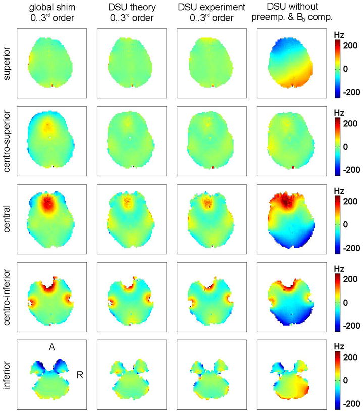
DSU and global shimming of the human brain at 7 Tesla. First column: Considerable field variation remains after static, global zero- to third-order SH shimming. Second column: The theoretical, slice-by-slice removal of zero- to third-order terms predicts largely improved shimming with DSU. Third column: Experimental field maps after DSU with preemphasis and B₀ compensation are virtually identical to the theoretical predictions. Forth column: The application of the same DSU settings without preemphasis and B₀ compensation leads to strong eddy-current induced field artifacts that abolish the benefits of DSU. See text for details.

Table 2.

Experimental whole brain zero - to third - order global shimming and DSU of 5 human subjects at 7 Tesla.

Measure	3rd Order Static, Global Shim							3rd Order DSU
	Subject					Mean	S.D.	Subject					Mean	S.D.
	1	2	3	4	5			1	2	3	4	5
80%	72.3	68.3	52.2	60.2	72.3	65.1	8.7	52.2	52.2	40.2	48.2	64.3	51.4	8.7
85%	92.4	84.3	64.3	80.3	84.3	81.1	10.4	64.3	60.2	48.2	56.2	72.3	60.2	9.0
90%	124.5	116.5	88.4	108.4	104.4	108.4	13.6	80.3	76.3	60.2	72.3	84.3	74.7	9.2
95%	224.9	168.7	132.5	164.7	152.6	168.7	34.4	112.4	104.4	88.4	116.5	108.4	106.0	10.8
98%	305.2	224.9	224.9	269.1	241.0	253.0	34.3	168.7	148.6	128.5	176.7	160.6	156.6	18.8
99%	393.6	297.2	301.2	309.2	325.3	325.3	39.7	216.9	196.8	196.8	245.0	180.7	207.2	24.7
S.D.	44.4	38.3	31.7	39.7	37.9	38.4	4.6	29.2	25.9	22.5	28.8	28.7	27.0	2.8
FWHM	23.5	25.9	15.0	18.6	15.9	19.8	4.8	17.2	13.9	28.8	24.8	13.8	19.7	6.8

Quantitative measures of the residual magnetic field inhomogeneities after shimming (in Hertz) include the frequency span to cover 80% to 99% of the voxels, as well as the standard deviation (S.D.) and the full width at half maximum (FWHM) of the frequency distribution.

The results summarized in Table 2 show that DSU clearly outperformed global, static shimming (of the same SH order) in all 5 subjects and considerably reduced residual magnetic field distortions. In particular DSU was capable of largely limiting the amount of high frequency distortion areas caused by the nasal and auditory cavities which is reflected by the 21% to 38% reduction of the frequency spans including 85 to 99% of the brain voxels. The application of zero- to third-order DSU with full preemphasis and B₀ compensation consistently reduced the whole brain standard deviation of the voxel frequencies in all subjects with an average improvement of 30%. Only the FWHM of the frequency distributions, which is dominated by the bulk voxels, remained effectively unaltered due to concomitant changes of the line shape.

DISCUSSION

Shimming of the human brain at 7 Tesla benefits from DSU compared to a singular, static adjustment of global shim values. However, the multitude of unwanted, temporally varying magnetic fields arising from eddy-currents related to dynamic application of shim fields can strongly degrade the magnetic field homogeneity if not compensated properly. Without preemphasis and B₀ compensation, strong random field variations were observed. They were mostly linear, but higher order terms were not negligible and preemphasis and B₀ compensation have to be considered essential requisites for a successful implementation of higher-order DSU. Active shielding, as shown here for Z2, does minimize eddy currents, as expected. However, active shielding of all 16 SH coils while retaining sufficient strength appears currently not feasible.

Image-based methods for the spatio-temporal characterization of eddy-currents are very time consuming due to the multitude of sampling time points and the number of SH terms considered. A quantitative and non-iterative calibration method has been presented that allows the efficient measurement of temporal SH shim-to-shim interactions along 1D column projections. The decomposition of the temporal eddy-current behavior for each of the 16 zero- to third-order shim coils into up to 3 exponentials allowed full preemphasis and B₀ compensation of all 16 shims covering 67 potential shim-to-shim interactions. When electronic control of the preemphasis circuitry is available, the presented method has the potential to become fully automated, with little or no user interaction.

The thorough characterization of the inherent static properties of the shim system is considered key for the successful application of DSU. Besides the measurement of the magnetic fields of the SH terms that are generated by the corresponding SH coils, i.e. the direct calibration of the SH coils, a comprehensive calibration of the shim system must also include the characterization of unwanted (static) SH cross-terms. In this study, all 16 zero- to third-order terms for all DSU brain slices were derived from a single reference field map and multiple iterations like in (27) were not necessary.

The experimental realization of preemphasis requires the dedication of part of the shim systems’ dynamic range to the compensation of the switching imperfections. Effective DSU shim strengths were sufficient in this study to achieve dynamically updated zero- to third-order magnetic field homogenizing of all considered axial brain slices at 7 Tesla. The shim requirements were defined by the shape, size and position of the magnetic field artifacts. Besides the subject anatomy, the head positioning could play a significant role (28). In particular, the backward tilt of the subjects’ head caused the positive field foci to move from the center of the prefrontal cortex to its frontal end. Shim settings were considerably different if the positive lobe of the prefrontal field artifact was no longer fully surrounded by a ring of low-field brain tissue, but located at the border of the brain.

The fast and reliable extraction of magnetic field distributions from human brain slices, i.e. the selection of shim volumes, is essential for successful DSU. A combination of algorithms and conditions was used in this study for brain extraction that did not only include anatomy or image criteria, but also applied quality-based measures such as an error threshold for the voxel-specific frequency calculation. The determination of slice-specific shim values for DSU comprising image reconstruction, field map calculation and DSU analysis for all slices took less than 1 minute on a regular PC. Multi-slice field mapping was used in this study to prove the quality of DSU, however, DSU does not rely in any way on the selected MR method and can be applied with any multi-volume imaging or spectroscopy sequence.

The definition of magnetic field homogeneity is straightforward, but the quantification and evaluation of magnetic field inhomogeneity is not. DSU proved particularly useful for the minimization of strong magnetic field variations such as the positive and negative patterns originating from the nasal cavities (compare Fig. 3). The impact of magnetic field homogeneity is highly pulse sequence dependent and therefore different approaches at optimization were examined. The direct least-squares approximation of magnetic field distortions with SH fields as applied in this study minimized the standard deviation of the frequency residual of the considered voxel ensemble. This approach considers all voxels, is robust and the standard method for the determination of shim fields as well as the evaluation of magnetic field homogeneity (27,29,30). Alternatively, an approach was implemented that derived the SH shim settings through minimization of the brain’s voxel-to-voxel magnetic field gradients similar to the method used by Cusack et al. (10). Determined shim settings, however, closely resembled the results derived through minimization of magnetic field variations and the deviations were typically well below 5% of the dynamic range of the shim system (data not shown). Although magnetic field variations and local gradients are not the same, the observation can be understood from the fact that they are nevertheless inherently correlated. Explicit focusing of the shim procedure on the major field distortions by spatial or frequency (i.e. field) weighting can further reduce the number of voxels with high amplitude field deviations. These approaches, however, come at the price of minor or major degradation of the magnetic field homogeneity in other brain areas based on the emphasis level. The concomitant impairment of frequency measures such as the standard deviation can be acceptable, for instance, if one solely aims to push local gradients for all voxels below the sequence-specific threshold for signal cancellation in, for example, gradient echo EPI. For other applications such as MR spectroscopy or spectroscopic imaging, increased magnetic field alterations over large parts of the brain may not always be an option.

Although the increased magnetic field inhomongeneity at 7 Tesla benefits from inclusion of third-order shims during DSU the magnetic field homogeneity is still not perfect, however, even with zero- to third-order DSU. It has been shown in this study that remaining field variations are not due to inaccurate implementation of DSU, but they are due to the shallowness of the applied low-order SH shim fields and therefore inherent to the method (Fig. 3, center columns). However, DSU maximizes the usefulness of conventional shim coil systems and provides magnetic field homogeneity that is adequate for a wide range of applications. Figure 4A shows a selection of two theoretically calculated, representative frequency span measures at 7 Tesla. The measures are averaged over the 5 subjects of this study and presented as a function of the SH order for global shimming (black) and DSU (gray). The standard deviations are shown as error bars.

FIGURE 4.

Theoretical comparison of DSU and static global shimming of the human brain at 7 Tesla as a function of SH shim order. (A) Improvements of the magnetic field homogeneity, equivalent to reduced frequency measures, are achieved with DSU (gray) compared to global shimming (black) at all SH orders. Although differences of the absolute frequency measures (in Hertz) are strongly affected by the applied inhomogeneity criteria, the relative functional behavior is similar for higher-order (n > 1) shimming. Combined measures comprise the average of all frequency measures, while error bars indicate the corresponding standard deviations. (A) The shim performance, i.e. the relative improvement of the field inhomogeneity measures, enhances as a function of SH order (solid lines), but relative performance gains with the inclusion of additional SH orders become small for the inclusion of third or even higher SH orders. See text for details.

The frequency measures for the quantification of magnetic field inhomogeneity improve with the inclusion of higher order SH terms, notably starting already with the slice-specific adjustment of B₀ offsets. The absolute reduction is bigger for frequency spans to cover larger percentages of the considered brain voxels. For the span covering 98% of the voxels (Fig. 4A, solid lines) and for SH orders n > 1 the difference between static global shimming and DSU stabilizes in the 110–115 Hz range. The frequency span covering 85% of the brain voxels shows the same functional behavior, although with smaller absolute improvements (Fig. 4A, dashed lines). It has been shown in this study that slice-selective zero- to third-order DSU provided improved magnetic field homogenization of the human brain when compared to the global adjustment of the same shim terms. Figure 4A furthermore shows that global zero- to third-order shimming of the human brain is already outperformed by zero- to second-order DSU. Pushing standard second-order shim coils to their maximum performance by DSU, therefore, is more beneficial for shimming the human brain than the extension of the coil system by a full set of third-order coils for global shimming. In fact, magnetic field homogenization with second-order DSU can compete with fourth- and maybe even fifth-order global shimming.

A multitude of factors has to be considered to assess the impact of the residual field imperfections on the MR data quality after global shimming and DSU at a given SH order in order to make the best decision on which shim system to install. MR sequence-specific requirements (e.g. gradient echo EPI versus spectroscopic imaging) play an important role; however, such detailed discussion is well beyond the scope of this publication. Instead, shim performances were calculated as the average improvement over all frequency measures and all subjects, and referenced to global third-order SH shimming (Fig. 4B, solid lines). Both, global shimming and DSU performances show a largely linear dependency on the SH shim order. The bigger slope of DSU reflects the inherently better utilization of SH field terms when dynamically applied to smaller volumes.

Despite the obvious benefits with the inclusion of higher SH orders, in practice, limitations in space, financial resources, available electronics (e.g. for preemphasis and B₀ compensation) or limited expertise have to be considered. The relative performance, i.e. the performance gain with the installation of the next higher SH order, therefore, can be a valuable measure for the benefits of a system upgrade (Fig. 4B, dashed lines). The relative performance of a given order for DSU or global shimming was calculated by comparing the performance at a given SH order with the performance of the same method at the next lower SH order. While major performance improvements are achieved by inclusion of first- and second-order terms for DSU, relative improvements become smaller for the consideration of higher, i.e. third, fourth and fifth SH orders. Notably, the largest gain in performance with global shimming is achieved by adding second-order SH terms, while the inclusion of first-order SH terms is the most beneficial step for DSU. The experimental realization of full preemphasis and B₀ compensation for zero- to third-order DSU as presented in this study has been a challenge. Effort and complexity of even higher-order DSU will be disproportionally higher. Although there is no principle reasons against fourth- or even higher-order DSU, the progressively smaller additional benefits per SH order can hardly justify the more predominant, concomitant downsides.

To date, the theoretical gains of high field (functional) MR imaging and spectroscopy have only been realized partially due to the elevated magnetic field distortions at higher field and limited shimming. The first realization of DSU of the human brain at 7 Tesla using all zero- to third-order shims with full preemphasis and B₀ compensation between all shim orders will allow considerably improved quality of imaging, spectroscopy and spectroscopic imaging applications in the human brain at 7 Tesla.

References

- 1.Golay MJE. Field Homogenizing Coils for Nuclear Spin Resonance Instrumentation. Rev Sci Instrum. 1958;29:313–315. [Google Scholar]
- 2.Romeo F, Hoult DI. Magnet field profiling: analysis and correcting coil design. Magn Reson Med. 1984;1:44–65. doi: 10.1002/mrm.1910010107. [DOI] [PubMed] [Google Scholar]
- 3.de Graaf RA. In Vivo NMR Spectroscopy: Principles and Techniques. London: John Wiley and Sons; 2008. pp. 494–497. [Google Scholar]
- 4.Gruetter R, Boesch C. Fast, Noniterative Shimming of Spatially Localized Signals. In Vivo Analysis of the Magnetic Field along Axes. J Magn Reson. 1992;96:323–334. [Google Scholar]
- 5.Gruetter R. Automatic, localized in vivo adjustment of all first- and second-order shim coils. Magn Reson Med. 1993;29:804–11. doi: 10.1002/mrm.1910290613. [DOI] [PubMed] [Google Scholar]
- 6.Shen J. Effect of degenerate spherical harmonics and a method for automatic shimming of oblique slices. NMR Biomed. 2001;14:177–83. doi: 10.1002/nbm.691. [DOI] [PubMed] [Google Scholar]
- 7.Zhang Y, Li S, Shen J. Automatic high-order shimming using parallel columns mapping (PACMAP) Magn Reson Med. 2009;62:1073–9. doi: 10.1002/mrm.22077. [DOI] [PMC free article] [PubMed] [Google Scholar]
- 8.Wilson JL, Jenkinson M, Jezzard P. Optimization of static field homogeneity in human brain using diamagnetic passive shims. Magn Reson Med. 2002;48:906–14. doi: 10.1002/mrm.10298. [DOI] [PubMed] [Google Scholar]
- 9.Wilson JL, Jezzard P. Utilization of an intra-oral diamagnetic passive shim in functional MRI of the inferior frontal cortex. Magn Reson Med. 2003;50:1089–94. doi: 10.1002/mrm.10626. [DOI] [PubMed] [Google Scholar]
- 10.Cusack R, Russell B, Cox SM, De Panfilis C, Schwarzbauer C, Ansorge R. An evaluation of the use of passive shimming to improve frontal sensitivity in fMRI. Neuroimage. 2005;24:82–91. doi: 10.1016/j.neuroimage.2004.08.029. [DOI] [PubMed] [Google Scholar]
- 11.Hsu JJ, Glover GH. Mitigation of susceptibility-induced signal loss in neuroimaging using localized shim coils. Magn Reson Med. 2005;53:243–8. doi: 10.1002/mrm.20365. [DOI] [PubMed] [Google Scholar]
- 12.Juchem C, Muller-Bierl B, Schick F, Logothetis NK, Pfeuffer J. Combined Passive and Active Shimming for In Vivo MR Spectroscopy at High Magnetic Fields. J Magn Reson. 2006;183:278–289. doi: 10.1016/j.jmr.2006.09.002. [DOI] [PubMed] [Google Scholar]
- 13.Juchem C, Nixon TW, McIntyre S, Rothman DL, de Graaf RA. Magnetic field homogenization of the human prefrontal cortex with a set of localized electrical coils. Magn Reson Med. 2010;63:171–180. doi: 10.1002/mrm.22164. [DOI] [PMC free article] [PubMed] [Google Scholar]
- 14.Blamire AM, Rothman DL, Nixon T. Dynamic shim updating: a new approach towards optimized whole brain shimming. Magn Reson Med. 1996;36:159–65. doi: 10.1002/mrm.1910360125. [DOI] [PubMed] [Google Scholar]
- 15.Morrell G, Spielman D. Dynamic shimming for multi-slice magnetic resonance imaging. Magn Reson Med. 1997;38:477–83. doi: 10.1002/mrm.1910380316. [DOI] [PubMed] [Google Scholar]
- 16.de Graaf RA, Brown PB, McIntyre S, Rothman DL, Nixon TW. Dynamic shim updating (DSU) for multislice signal acquisition. Magn Reson Med. 2003;49:409–16. doi: 10.1002/mrm.10404. [DOI] [PubMed] [Google Scholar]
- 17.Koch KM, McIntyre S, Nixon TW, Rothman DL, de Graaf RA. Dynamic shim updating on the human brain. J Magn Reson. 2006;180:286–96. doi: 10.1016/j.jmr.2006.03.007. [DOI] [PubMed] [Google Scholar]
- 18.Koch KM, Brown PB, Rothman DL, de Graaf RA. Sample-specific diamagnetic and paramagnetic passive shimming. J Magn Reson. 2006;182:66–74. doi: 10.1016/j.jmr.2006.06.013. [DOI] [PubMed] [Google Scholar]
- 19.Juchem C, Nixon TW, McIntyre S, Rothman DL, de Graaf RA. Magnetic Field Modeling with a Set of Localized Individual Coils. J Magn Reson. 2010 doi: 10.1016/j.jmr.2010.03.008. in press. [DOI] [PMC free article] [PubMed] [Google Scholar]
- 20.Juchem C, Nixon TW, Diduch P, McIntyre S, Rothman DL, Starewicz P, de Graaf RA. Zero- to Third-Order Dynamic Shim Updating of the Human Brain at 7 Tesla. Stockholm; Sweden: 2010. p. 222. [Google Scholar]
- 21.Jensen DJ, Brey WW, Delayre JL, Narayana PA. Reduction of pulsed gradient settling time in the superconducting magnet of a magnetic resonance instrument. Med Phys. 1987;14:859–62. doi: 10.1118/1.596012. [DOI] [PubMed] [Google Scholar]
- 22.van Vaals JJ, Bergman AH. Optimization of eddy-current compensation. J Magn Reson. 1990;90:52–70. [Google Scholar]
- 23.Terpstra M, Andersen PM, Gruetter R. Localized eddy current compensation using quantitative field mapping. J Magn Reson. 1998;131:139–43. doi: 10.1006/jmre.1997.1353. [DOI] [PubMed] [Google Scholar]
- 24.Vaughan JT, Hetherington HP, Otu JO, Pan JW, Pohost GM. High frequency volume coils for clinical NMR imaging and spectroscopy. Magn Reson Med. 1994;32:206–18. doi: 10.1002/mrm.1910320209. [DOI] [PubMed] [Google Scholar]
- 25.Smith SM. Fast robust automated brain extraction. Hum Brain Mapp. 2002;17:143–55. doi: 10.1002/hbm.10062. [DOI] [PMC free article] [PubMed] [Google Scholar]
- 26.Wen H, Jaffer FA. An in vivo automated shimming method taking into account shim current constraints. Magn Reson Med. 1995;34:898–904. doi: 10.1002/mrm.1910340616. [DOI] [PMC free article] [PubMed] [Google Scholar]
- 27.Miyasaka N, Takahashi K, Hetherington HP. Fully automated shim mapping method for spectroscopic imaging of the mouse brain at 9.4 T. Magn Reson Med. 2006;55:198–202. doi: 10.1002/mrm.20731. [DOI] [PubMed] [Google Scholar]
- 28.Tyszka JM, Mamelak AN. Quantification of B0 homogeneity variation with head pitch by registered three-dimensional field mapping. J Magn Reson. 2002;159:213–8. doi: 10.1016/s1090-7807(02)00101-5. [DOI] [PubMed] [Google Scholar]
- 29.Spielman DM, Adalsteinsson E, Lim KO. Quantitative assessment of improved homogeneity using higher-order shims for spectroscopic imaging of the brain. Magn Reson Med. 1998;40:376–82. doi: 10.1002/mrm.1910400307. [DOI] [PubMed] [Google Scholar]
- 30.Wilson JL, Jenkinson M, de Araujo I, Kringelbach ML, Rolls ET, Jezzard P. Fast, fully automated global and local magnetic field optimization for fMRI of the human brain. Neuroimage. 2002;17:967–76. [PubMed] [Google Scholar]