DomSVR: domain boundary prediction with support vector regression from sequence information alone

Abstract

Protein domains are structural and fundamental functional units of proteins. The information of protein domain boundaries is helpful in understanding the evolution, structures and functions of proteins, and also plays an important role in protein classification. In this paper, we propose a support vector regression-based method to address the problem of protein domain boundary identification based on novel input profiles extracted from AAindex database. As a result, our method achieves an average sensitivity of ~36.5% and an average specificity of ~81% for multi-domain protein chains, which is overall better than the performance of published approaches to identify domain boundary. As our method used sequence information alone, our method is simpler and faster.

Introduction

Protein domains are importantly independent units of protein tertiary structures and have been studied extensively in recent decades. Edelman et al. studied the structures of immunoglobulins and first proposed some important hypothesizes on domain structures (Edelman 1973; Porter 1973). Wetlaufer (1973) subsequently proposed the concept of domain and defined domains as stable, compact, and autonomously folding structures of proteins based on a thorough investigation of immunoglobulins. A domain can span an entire polypeptide chain or be a subunit of a chain which can be folding into a stable tertiary structure independently (Levitt and Chothia 1976).

Typically, most domains have a single continuous polypeptide segment, while a few others consist of several discontinuous segments. Furthermore, many protein chains consist of more than one structural domains, all of them form independently compact structures (Wetlaufer 1973). Moreover, it is observed that a large protein may get its optimal protein folding by domain formation, when giving an observed random distribution of hydrophobic residues in large proteins (George and Heringa 2002a, b). Actually, each domain contains an individual hydrophobic core that is built from secondary structures (Zhou et al. 1999). Residues in hydrophobic core are more conserved than residues at the surface in a protein family unless the latter are involved in the functions of the protein (Zhou et al. 1999).

Previous works on the prediction of protein domain boundaries are roughly classified into two categories: template-based methods (Altschul et al. 1997; Cheng et al. 2006; Gewehr and Zimmer 2006; Marchler-Bauer et al. 2007; Marsden et al. 2002; Orengo et al. 1997) and ab initio methods (Copley et al. 2002; Dumontier et al. 2005; Galzitskaya and Melnik 2003; George and Heringa 2002b; Nagarajan and Yona 2004; Sikder and Zomaya 2006; Sim et al. 2005; Suyama and Ohara 2003). Template-based methods aim to predict domain boundaries using sequence alignment (Marchler-Bauer et al. 2007), secondary structure alignment (Cheng et al. 2006; Marsden et al. 2002), or other profile alignments. They align target profiles against profiles in a domain database. Among template-based methods, conserved domain database (CDD) (Marchler-Bauer et al. 2007) locates residues in domain boundaries using a search tool, reverse position-specific BLAST (RPS-BLAST). With CDD method, firstly, query sequences are compared to databases of position-specific scoring matrices (PSSMs). Secondly, E values are obtained in much the same way as in the PSI-BLAST application (Altschul et al. 1997). Overlapping domain hits are finally obtained by the sort of the E values. DomSSEA (Marsden et al. 2002) predicts domain boundaries by aligning the predicted secondary structures of target sequences against a database of observed secondary structures of chains that have known domain boundaries (Orengo et al. 1997). SSEP-Domain method predicts domains with the alignment information of secondary structures and profile–profile as well as pattern searches (Gewehr and Zimmer 2006).

Most ab initio methods aim to identify protein domain boundaries based on the information of the properties of residues in protein chains using various machine learning techniques. Among them, CHOPnet addresses some issues in domain annotation with evolutionary information, amino acid composition, and amino acid flexibility (Copley et al. 2002); SnapDRAGON predicts domain boundaries using a distance geometry-based folding technique with a 3D domain assignment algorithm (George and Heringa 2002b); Galzitskaya and Melnik (2003) propose a simple approach to identify domain boundaries in proteins using side chain entropy of a residue region; DomCut’s method predicts inter-domain linker regions using amino acid sequence information (Suyama and Ohara 2003); Nagarajan and Yona (2004) propose a neural network-based method to detect domain structure of a protein, which uses the information from multiple sequence alignments analysis, position-specific properties of amino acids, and predicted secondary structures; PRODO (Sim et al. 2005) uses a neural network method with information from position-specific scoring matrix (PSSM) generated by PSI-BLAST (Altschul et al. 1997); Armadillo aims to predict domain boundaries by converting protein sequences to smoothed numeric profiles based on domain linker propensity index (DLI) from amino acids’ composition (Dumontier et al. 2005); Dovidchenko et al. (2007) propose a simple and fast method with the use of a minimal number of amino acid sequence alone; DomainDiscovery detects domain boundaries by the use of support vector machines with sequence information including a PSSM, secondary structure, solvent accessibility information and inter-domain linker index (Sikder and Zomaya 2006); DOMpro applies recursive neural network to predict domain boundaries with evolutionary information, solvent evolutionary information, solvent accessibility information, and secondary structure (Cheng et al. 2006); Ye et al. (2007) present a Back-Propagation (BP) neural network approach to predict the domain boundaries with various property profiles; recently, Yoo et al. (2008) develop a new improved general regression network (IGRN) model to detect domain boundaries using a PSSM, secondary structure, information, and inter-domain linker index.

However, the accuracy of predicting multi-domain boundaries is considerably less than 40% in spite of great development on domain boundary prediction in the past years by the use of a large number of machine learners. Therefore, novel machine learning-based approaches should be developed to accurately identify protein domain boundaries.

Most previous work in the prediction of domain boundaries has been on the so-called “classification problem”. In this case, residues are assigned to one of two states, domain boundary or non-domain boundary, with arbitrary cutoff thresholds. However, the selection of thresholds is neither objective nor optimal, and the decomposition of residues into two classes decreases the prediction accuracy. To overcome such disadvantages, we predict domain boundary value for each residue. That is, our method predicts a series of real values representing residues in a protein sequence (also regarded as the boundary profile). In this paper, we develop an accurate, fast, and reliable ab initio protein domain boundary predictor, named as DomSVR, by the use of support vector regression (SVR) starting from protein sequence alone. The method just uses profiles extracted from AAindex database (Kawashima et al. 2008). Our proposed method DomSVR achieves an average sensitivity of ~36.5% and an average specificity of ~81% for multi-domain protein chains, which is overall better than the performance of published approaches to identify domain boundary. As our method used sequence information alone, our method is simpler and faster.

Methods

Dataset preparation

Our model is trained and tested on the dataset extracted from DOMpro method (Cheng et al. 2006). In this paper, we only consider proteins with more than one domain. Finally, 354 multi-domain proteins are used to evaluate our proposed method of protein domain boundary prediction. In the dataset, sequence identity of each two protein chains is less than 25%. Moreover, all protein chains contain more than 40 amino acid residues. The dataset consists of 282 two-domain chains, 50 three-domain chains, and 22 chains having more than three domains. The dataset can be found at our website: http://mail.ustc.edu.cn/~bigeagle/DomSVR/index.htm.

Creation of amino acid physicochemical profiles for inputs of SVR predictor

In this work, we encode input vectors of SVR predictor using amino acid profiles extracted from AAindex database (Kawashima et al. 2008). First, we need to assign physical and chemical properties to amino acid residues. Vectors of suitable amino acid physicochemical properties will then be created and be used for the domain boundary assignment. The physicochemical properties of amino acid residues include inter-residue contact energy, secondary structure, residue charge, and other properties. In addition, the simple forms of the vectors make the entire algorithm robust, fast, and easy to apply.

The AAindex database contains a large number of experimental indexes, representing a large variety of physicochemical and biological properties of the amino acids. The AAindex1 section of the amino acid index database collects published indices together with the result of cluster analysis using the correlation coefficient as the distance between two indices (Kawashima et al. 2008). The section currently contains 544 indices, excluding all empirically derived propensities of amino acids. Taking all these 544 amino acid properties as input features for a predictor may cause over-fitting. In order to distinguish and separate significant data and then construct our profile vectors, we applied principal component analysis (PCA) (Jolliffe 2002) on these properties. PCA is often used to reduce the dimensionality of a given dataset to lower dimensions for analysis. It can then produce a new set of principal components, which account for the top largest variations of the original data. PCA takes linear combinations of the data complying with the rule that the first principal component accounts for the maximum variation, the second principal component accounts for the next maximum variation which is subject to being orthogonal to the first one, the third one has the third maximum variation subject to being orthogonal to the first two, and so on. Nineteen principal components were created which account for 99.99% of the variance in the AAindex1 dataset. Among those components, the top four components account for 93.78% of the experimental data variation. Using only four principal component vectors as shown in Table 1, the entire original dataset of properties is described with an approximate 6.22% loss of variation. Thus, the dimensionality of the original data is significantly reduced. The first principal component, PrinComp1, which solely accounts for 55% of the data variation, has a strong correlation to inter-residue contact energy property (Miyazawa and Jernigan 1999). The second component, PrinComp2, is correlated to secondary structure propensities of amino acids (Munoz and Serrano 1994). The third component, PrinComp3, is correlated to entire chain composition of amino acids (Fukuchi and Nishikawa 2001). Finally, PrinComp4 is mainly correlated to conformational and nucleation properties of individual amino acids (Rackovsky and Scheraga 1982).

Table 1.

The top four principal component profiles and the variation account rates

Profile	A/R	N/D	C/Q	E/G	H/I	L/K	M/F	P/S	T/W	Y/V	Rate (%)
PrinComp1	−81.9	−280.1	460.7	−257	−19.5	220.1	316.3	−262.3	−44.8	125	51.01
	−269.3	−134.5	−277.7	−260.5	271.5	−350.2	408.9	−262.3	467.8	229.8
PrinComp2	357.2	−66.5	102.8	−101.2	−257.5	203.3	−140.9	−30.5	112.7	−178.2	25.45
	−276	−20.2	−209.1	377	74.5	−77.8	−30.3	189.5	−270	241.1
PrinComp3	−55.8	−86	214.8	150.6	−155	−67.1	−71	−187.4	155.4	−76.3	10.09
	−18.4	243	−16.3	−105.7	−82	212.6	−35.8	−44.1	10.6	13.8
PrinComp4	−26.8	55.2	209.6	−3.4	98.9	−179.4	100.1	151.9	31.1	−104.4	7.23
	−137.6	95.3	51.3	48.7	−58.3	−185.6	−67.8	28.5	−28.3	−78.9

Each principal component profile needs to be equalized by normalized itself when applying to create input vectors for SVR predictor

For protein chain with L residues, in the case of Prin-Comp1 profile, each residue is encoded as the central residue in a sliding window with nine residues along the peptide chain. Then, the central residue is represented by a 1 × 9 vector, and the value for each element of the vector corresponds to specific amino acid type in PrinComp1. Therefore, the protein chain is represented by a L × 9 matrix which corresponds to a real value vector L × 1, where each residue is assigned to a real value that measures the sequence distance between the residue and the central residue of its closest domain boundary.

The targets of SVR predictor

The identification of domain boundaries for each protein chain can be viewed as a binary regression problem. Each residue along the polypeptide chains is encoded by AAindex amino acid profiles and assigned a real target value. Following the conventions used in prior work (Cheng et al. 2006; Liu and Rost 2004; Marsden et al. 2002), suppose that residues within more than 20 continuous amino acids of a domain boundary are regarded as domain boundary residues, and non-domain boundary residues otherwise.

Actually SVR is particularly suitable for solving such regression problem. Assigned real value to a residue as target can be more efficient and effective than the assignment of classification value 1 or 0 as target. In this work, a residue is assigned to a domain boundary (DB) value, which measures the residue distancing away from its closest domain boundary in sequence. The assignment for residue i is shown in the following form:

$${\text{DB}}_i=\{\begin{array}{ll}\frac{{\text{cb}}_m-\mid i-{\text{cb}}_m\mid }{{\text{cb}}_m}\hfill & \text{if}i\text{in}\text{boundary}\hfill \\ -\frac{\mid i-r_{\text{end}}\mid }{r_{\text{end}}-r_{\text{start}}}\hfill & \text{if}i\text{in}\text{non}-\text{boundary}\text{near}\text{the}\text{N}-\text{termini}\hfill \\ -\frac{\mid i-r_{\text{start}}\mid }{r_{\text{end}}-r_{\text{start}}}\hfill & \text{if}i\text{in}\text{non}-\text{boundary}\text{near}\text{the}\text{C}-\text{termini}\hfill \\ -\frac{{\text{cnb}}_n-\mid i-{\text{cnb}}_n\mid }{{\text{cnb}}_n}\hfill & \text{Otherwise}\hfill \end{array},$$ (1)

where DB_i denotes the DB value for residue i, cb_m indicates the sequence position of central residue m in domain boundary cb if cb existed, cnb_n means the sequence position of central residue n in non-boundary cnb, while r_start and r_end stand for the sequence positions of the starting and the end residues in the non-boundary sequence, respectively.

The form of Eq. 1 is a triangular distribution with respect to residue position in primary sequence. Central residue in domain boundary is assigned to a bigger value, while the more far away from the boundary the more small value the residue is assigned to. Finally, the target vector DB also needs to be normalized to equalize itself.

For each residue in protein chains, in summary, vector to be input into SVR is represented as an array X_i, where each element in the array corresponds to amino acid type of each AAindex profile, while the corresponding target DB_i is another real value which is assigned by Eq. 1 in terms of the sequence distance between residue i and its closest domain boundary. Similar to most other machine learners, DomSVR method aims to learn the mapping from the input array X onto the corresponding target array DB. Suppose that O is an output array of SVR, DomSVR is trained to make the output O as close as possible to the target DB.

Approach

Support vector regression aims to apply support vector machine to regression problems by introducing an alternative loss function. Likely as SVM approach (Chen et al. 2007), linear regression of SVR is performed in a high-dimensional feature space mapped from complex data with a non-linear mapping (Gunn 1998). With SVR, a ε-insensitive loss function is used where only errors greater than a predefined parameter ε are considered in the loss function. Readers can refer to (Drucker et al. 1996; Gunn 1998) for more details.

Consider the problem of learning a set of data, (X_i, DB_i), such that X_i ∈ ℜⁿ is an input vector which characterizes a residue along protein chains, and DB_i ∈ ℜ is a real target value which represents its associated boundary value measuring the separation between the residue i and the closest domain boundary in sequence, with a linear function,

$$f(X)=\langle w,X\rangle +b.$$ (2)

The optimized parameters w and b can be obtained by minimizing the following objective function:

$$Ø(w,\xi )=\frac{1}{2}{\left|\right|w\left|\right|}^2+C\sum _i({\xi }_i^{-}+{\xi }_i^{+}).$$ (3)

where C is a regularization constant that balances training errors and model complexity, and ξ⁻ and ξ⁺ are slack variables representing upper and lower constraints which used to measure the deviation of samples outside the ε-insensitive zone.

In this work, we adopt an ε-insensitive loss function,

$$L_{\epsilon }(\text{DB})=\{\begin{array}{ll}0\hfill & \text{if}\mid f(X)-\text{DB}\mid <\epsilon \hfill \\ \mid f(X)-\text{DB}\mid -\epsilon \hfill & \text{Otherwise}\hfill \end{array}$$ (4)

To solve the optimization problem, therefore, two Lagrange multipliers α_i and ${\alpha }_i^{\ast }$ are applied and the solution is given by

$$\begin{array}{l}\text{Maximize}-\frac{1}{2}{\sum }_{i=1}^L{\sum }_{j=1}^L({\alpha }_i-{\alpha }_i^{\ast })({\alpha }_j-{\alpha }_j^{\ast })Q_{ij}+{\sum }_{i=1}^L{\alpha }_i({\text{DB}}_i-\epsilon )-{\alpha }_i^{\ast }({\text{DB}}_i+\epsilon )\\ \text{subject}\text{to}0\le {\alpha }_i,{\alpha }_i^{\ast }\le C,i=1,\dots ,L\\ \text{and}{\sum }_{i=1}^L({\alpha }_i-{\alpha }_i^{\ast })=0.\end{array}$$ (5)

where Q_ij = K(x_i, x_j)≡∅(x_i)^T ∅ (x_j).

Finally the decision function is

$$\sum _{i=1}^L({\alpha }_i-{\alpha }_i^{\ast })K(X_i,X)+b.$$ (6)

Once the Lagrange multipliers α_i and ${\alpha }_i^{\ast }$ and the bias b are determined from the training data, Eq. 6 can be applied to predict the domain boundary values for a test protein chain.

As a result, our model infers the domain boundary regions from predictions of domain boundary values for a test protein chain. The larger the prediction value is, the more possible the corresponding residue is belonging to domain boundary. In this work, a series of continuous residues are considered to be in domain boundary if the residue amount is more than 20 and their DB values are larger than other neighboring ones. At the same time, a series of continuous residues with bigger DB values are ignored if the residue amount is less than 5. Moreover, two inferred boundary regions that separate less than 10 residues should be merged into one region. The test chain is then cut into domain regions linked by boundary region (regions).

Evaluation measures

To evaluate our method, three measurements are used to evaluate the performance of the predictor: criteria of sensitivity (Sen), specificity (Spec), and accuracy (Acc) (Baldi et al. 2000; Saini and Fischer 2005). They are defined as follows:

$$\text{Sen}=\frac{\text{TP}}{\text{TP}+\text{FN}},\text{Spec}=\frac{\text{TP}}{\text{TP}+\text{FP}},\text{Acc}=\frac{\text{TP}+\text{TN}}{{\text{N}}_{\text{total}}}$$ (7)

where TP denotes the number of true positives (residues in domain boundaries), FP denotes the number of false positives, TN stands for the number of true negatives (residues in non-domain boundaries), and N_total stands for the number of total residues.

When assessing predictor with respect to domain boundary, evaluation is based on the above measures of Sen and Spec and, for the assessment with respect to domain number, measure of accuracy is the ratio of the number of chains whose domain number was predicted correctly to that of total protein chains.

Results

Domain boundary distribution

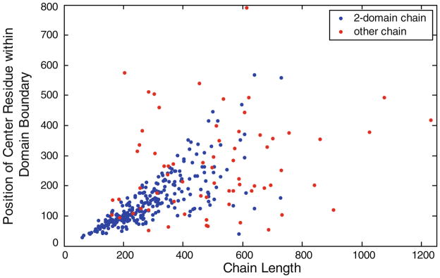
In this work, there are total 354 protein chains, each of which contains more than one domain. Figure 1 shows the distribution of sequence positions of residues at the center of domain boundaries. Most domain boundaries are far from the start and the end of the protein sequences. The distribution is helpful for limiting random noise of outputs from domain boundary prediction methods and further improves the identification rate of domain residues.

Fig. 1.

Distribution of sequence positions of residues at the center of domain boundaries. Blue dot denotes two-domain chain while red dot stands for protein chain containing more than two domains

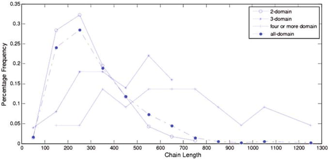
Figure 2 shows chain length distributions of multi-domain chains in the non-redundant set. From Fig. 2, the length distributions of multi-domain chains are not discrete, which has implications in domain prediction. As chain length increases, the likelihood of the chain having a multi-domain conformation almost increases. Most two-domain chains contain 100–200 amino acids. Most of three-domain chains contain 200–700 amino acids. Furthermore, chains containing more than 800 amino acid residues always have four or more domains.

Fig. 2.

Chain length distributions as observed in the CATH representative set used in this study. Intervals were calculated with a width of 100 residues. The domain frequencies were used to calculate probabilities of predicted domain sizes

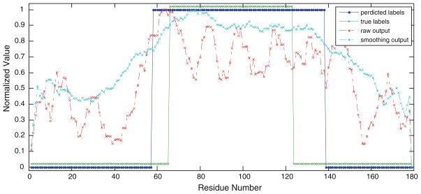
The output from domain boundary predictor is quite noisy. To limit random noises that come from false positive hits and false negative hits, smoothing technique is used to correct the random fluctuation of outputs for neighboring residues (Goodall 1990). The smoothing technique is accomplished by averaging over a window around each residue position. For instance, Fig. 3 shows a case study of prediction for protein chain PDB:1qu6A, where each residue is assigned a state (boundary/not boundary) by a cutoff threshold at 0.5 to the output of model. A residue will be assigned to 1 (boundary state) when the corresponding output is larger than the threshold and, 0 (not boundary state) otherwise. After smoothing the outputs for each residue, the center of the domain boundary was predicted at residue 80 and the domain number was also correctly predicted. Figure 3 also illustrates how smoothing technique helps reducing noises found in the raw outputs from the model. It is evident from Fig. 3 that the domain boundary threshold used to define the two classes (domain boundary and non-domain boundary) strongly affects the absolute classification results.

Fig. 3.

Comparison of raw and smoothing outputs from SVR model for protein chain 1qu6A. The protein chain has 179 residues and contains two domains lined by a domain boundary. The center of the domain boundary is at residue 94. The two types of outputs are normalized to the range [0, 1]. The two square curves denote the two kinds of residue labels. One is true labels describing residues’ states (boundaries/not boundaries); the other is predicted labels

Performance of the PCA profiles

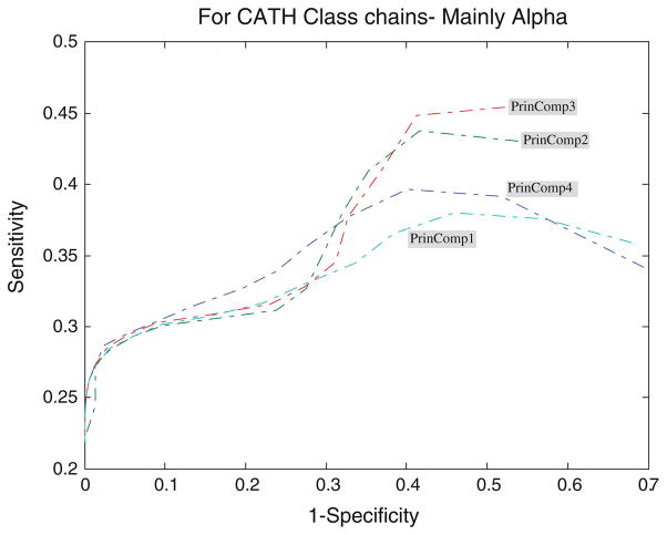
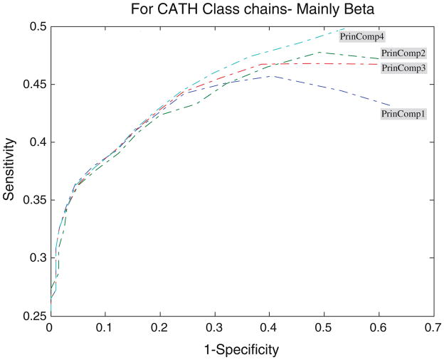
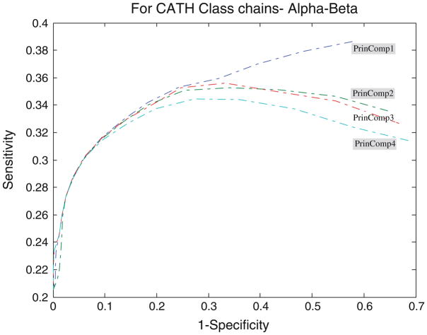
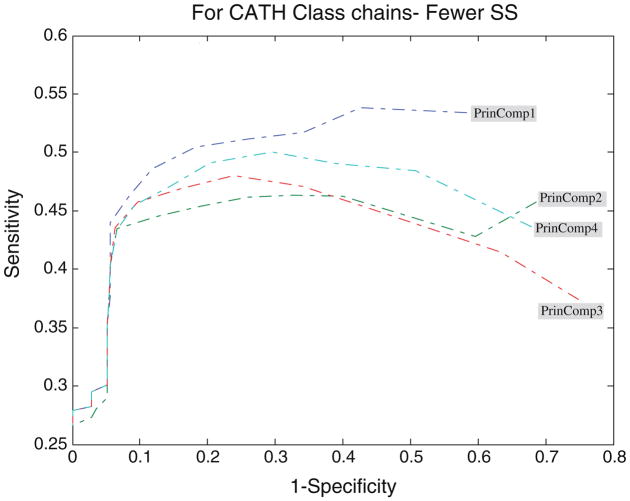
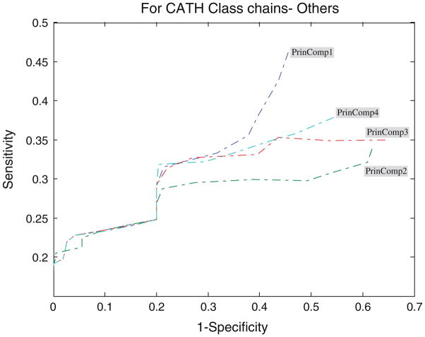
Figures 4, 5, 6, 7, and 8 show the ROC analysis of protein chains in CATH according to class membership, with the top four principal components being used as property descriptors. Based on CATH architecture, protein chains in our dataset are classified into four classes, i.e., mainly alpha, mainly beta, alpha and beta, and fewer secondary structure (SS). If all domains of a protein chain belong to one CATH class, the chain is classified into the same class. Inversely, if domains of a protein chain belong to different CATH classes, the chain is classified into class “Others”.

Fig. 4.

ROC analysis for mainly alpha proteins with respect to threshold

Fig. 5.

ROC analysis for mainly beta proteins with respect to threshold

Fig. 6.

ROC analysis for alpha–beta proteins with respect to threshold

Fig. 7.

ROC analysis for fewer secondary structures proteins with respect to threshold

Fig. 8.

ROC analysis for other proteins with respect to threshold

It is clearly shown that all the four profiles behave similar in their predictive ability. The average accuracy increases with the increase of the threshold, and all predictors reach high accuracy near the value of 0.7 for all protein classes. However, many key differences of their performance should be noted. An increase of the cutoff threshold positively affects performance of the domain boundaries prediction. The tradeoff for the increase of the sensitivity is the dramatic decrease of the specificity for almost all the four principal component profiles, as illustrated in Figs. 4, 5, 6, 7, and 8. In other words, from Eq. 7, the decrease of false domain boundary residues leads to the dramatic increase of false domain residues. In general, however, the decrease of the specificity (the same as the increase of the 1 – specificity being shown in the figures) will lead to the decrease of the sensitivity starting from a point in ROC curve. The point for mainly alpha proteins is near specificity 0.55 (i.e., 1 – specificity = 0.45), 0.6 for mainly beta proteins, 0.75 for alpha–beta proteins, and 0.7 for fewer SS proteins.

From Fig. 5 we can observe that for the set of mainly alpha proteins, PrinComp1 provides good predictions compared to other three profiles. This could be an indication that inter-residue contact energy is very important. Predictions using the first profile are also important for fewer SS proteins. Furthermore, predictions from PrinComp4 are important for mainly beta proteins but show poor prediction for alpha–beta proteins and all alpha proteins. PrinComp2 shows a much lower prediction performance for fewer SS proteins and other proteins.

It has also been observed that the sensitivities of predictions from PrinComp2 are the same as those from PrinComp3 for mainly alpha, mainly beta, and alpha–beta proteins in CATH. The specificities of predictions from PrinComp2 are the same as those from PrinComp1 for mainly alpha, mainly beta, and alpha–beta proteins in CATH. More importantly, all the four profiles show good predictions for mainly beta proteins compared to other proteins in CATH. The fewer SS proteins also show the same results although containing fewer numbers of proteins.

Performance with respect to protein classes

Tables 2 and 3 show the performance comparisons of the model on protein chains in our dataset classified by CATH and SCOP architectures, respectively. In the case of CATH architecture, protein chains are classified into seven classes in terms of the composition of secondary structure (SS), i.e., all alpha, all beta, alpha/beta, alpha + beta, multi-domain proteins, membrane and cell surface proteins, and small proteins. In this work, similar to the above discussion, all domains of a protein chain belonging to one SCOP class have the chain to be classified into the class. Inversely, all domains of a protein chain belonging to different SCOP classes may make the chain being classified into class “Other”.

Table 2.

Comparison of protein chains classified by CATH (%)

SS	No.	PrinComp1			PrinComp2			PrinComp3			PrinComp4
		Sen	Spec	Acc	Sen	Spec	Acc	Sen	Spec	Acc	Sen	Spec	Acc
Mainly alpha	40	32.9	76.2	63.7	31.7	72.5	62.6	31.8	72.6	62.8	32	729	62.8
Mainly beta	95	41.6	80.1	68.1	41.4	80	67.9	41.6	80.6	68.3	41.7	80.8	68.3
Alpha + beta	194	33.2	81.6	65.4	33	81.6	65.2	33	81.1	65.1	32.7	80.3	64.9
Fewer SS	9	47.6	88.1	72.4	44.4	80	69.6	45.9	83.8	70.9	46.1	85.5	71.2
Others	16	30.6	78.6	64.8	28.5	72.7	63.7	30.4	78	64.8	30.9	79.7	65.1

Table 3.

Comparison of protein chains classified by SCOP (%)

SS	No.	PrinComp1			PrinComp2			PrinComp3			PrinComp4
		Sen	Spec	Acc	Sen	Spec	Acc	Sen	Spec	Acc	Sen	Spec	Acc
All alpha	6	34.9	72.3	63.6	33.2	67.6	62.1	33.3	67.8	62.3	33.3	67.8	62
All beta	36	37.5	83.6	67.3	37	82.9	67	37.5	84	67.4	37.9	84.9	67.8
Alpha/beta	80	28.4	84.1	64.2	27.6	82.4	63.7	27.7	82.6	63.5	27.3	81.5	63.1
Alpha + beta	85	34.5	78.3	65.6	34.4	78.9	65.5	34.6	78.6	65.7	34.5	78.1	65.6
Multi-domain	101	29.5	89.7	65.5	28.5	87.2	64.2	27.9	84.4	64.2	29.3	88.8	65.5
Membrane and cell	10	30.5	84.5	65	30.9	85.7	65.3	30.8	85.7	65.2	29.6	82.7	64.1
Small proteins	8	66.6	74.4	75	66.6	73.9	75	66.8	74.8	75.3	66.4	74.5	74.9
Others	28	41.3	100	72.6	41.3	100	72.6	41.3	100	72.6	41.3	100	72.6
Total	354	36.5	80.8	66.3	35.6	80	65.8	35.9	80	66	35.8	80	65.9

When being classified by SCOP, small protein chains, although having six members, show the best performance. The overall sensitivity and the accuracy are around 0.666 and 0.75 from all the four profiles. However, all beta proteins and alpha + beta proteins have the second best sensitivities and accuracies. Proteins in other classes have sensitivity and specificity of 0.413 and 1 from all the four profiles, respectively. It has also been observed that the sensitivities of predictions from PrinComp2 tend to be the same as those from PrinComp3 and PrinComp4 for all alpha, all beta, alpha/beta, alpha + beta proteins when being classified by SCOP database.

As a result, the PrinComp1 profile shows a good prediction for all proteins compared to the other three profiles. Moreover, predictions from PrinComp3 are very similar to those from PronComp4. The reason behind the similarity of the predictions between PrinComp3 and PrinComp4 is that even though the two profiles are correlated to entire chain composition of amino acids and conformational properties of individual amino acids, they may also share other physicochemical properties from the original 544 properties set in AAindex1 database. In general, using all the four principal components leads to higher prediction accuracy.

Not all protein chains demonstrate similar behavior in the domain boundary prediction. It is noted that for some chains such as 1tf3A and 1dx5I, DomSVR predicts a very few number of false positives and false negatives, which lead to higher sensitivity and specificity performance. For protein chains such as 1hf2B, 1cfb0, and 1jr3E, our method make bad predictions, close to zeros for sensitivities and specificities with all the four profiles.

The important conclusion from these figures and tables is that PrinComp1, which as stated above is related to inter-residue contact energy, provides the most reliable prediction. This is due to the fact that in general PrinComp1 has the largest domain boundaries of predictions compared to the other three profiles. The average sensitivity of predictions over all protein chains is 0.365 for PrinComp1, 0.356 for PrinComp2, 0.359 for PrinComp3, and 0.358 for Prin-Comp4; the average specificity of predictions for all protein chains is 0.808 for PrinComp1 and 0.8 over all other three profiles.

Accuracy for different chains comparison with other methods

Our DomSVR method aims to predict domain boundaries for protein chains containing more than one domain. However, it is also suitable for the identification of one-domain protein chain. To make the comparison with other methods, we trained DomSVR predictor on our dataset integrating with other 963 one-domain chains, and then evaluated it both with respect to one-domain chains and multi-domain chains on CAFASP-4 and CASP7 benchmark datasets. The experiments on one-domain proteins were similar to those on multi-domain proteins. The dataset of one-domain chains is also available at our website: http://mail.ustc.edu.cn/~bigeagle/DomSVR/index.htm.

The detailed comparison with other similar methods is shown in Table 4 based on the PrinComp1 profile. Table 4 shows 13 previous predictors evaluated in the Critical Assessment of Fully Automated Structure Prediction 4 (CAFASP-4) (Saini and Fischer 2005), where some statistical data are extracted from DOMpro paper (Cheng et al. 2006). The evaluation dataset of CAFASP-4 consists of 41 one-domain CASP6 targets and 17 two-domain CASP6 targets (58 targets in total). The targets in CA-FASP-4 dataset are divided into two main divisions: homology modeling and fold recognition targets. Twenty one-domain chains and 7 two-domains chains are homology modeling targets, and 21 one-domain chains and 10 two-domain chains are fold recognition targets. In the CAFASP-4, seven predictors belong to the category of template-based methods, which have an advantage due to this evaluation set contains only comparative modeling and fold recognition targets (no new fold targets). Our method achieves higher sensitivity and specificity than other ab initio predictors when averaging over all of the targets. Moreover, in spite of our model outperforms even better than some template-based methods such as ADDA, Inter-ProScan, and Dompred-Domssea, it performs worse than other template-based methods such as Dopro, SSEP-Domain, and Robetta-Ginzu.

Table 4.

Performance comparison with other methods on CAFASP-4 benchmark dataset

Predictor	1-Da		2-D		Al-D
	Sen	Spec	Sen	Spec	Sen	Spec
DomSVRb	0.8	0.9	0.34	0.78	0.67	0.87
ADDA (Heger and Holm 2003)b	0.85	0.73	0.18	0.33	0.66	0.67
Armadillob	0.1	1	0.24	0.18	0.14	0.31
Biozon (Nagarajan and Yona 2004)b	0.1	1	0.35	0.19	0.17	0.29
Dompred-DPS (Bryson et al. 2005)b	0.68	0.78	0.47	0.5	0.62	0.69
DOMprob	0.85	0.76	0.35	0.5	0.71	0.71
Globplot (Linding et al. 2003)b	0.83	0.71	0.18	0.6	0.64	0.7
Mateo (Lexa and Valle 2003)b	0.51	0.78	0.12	0.15	0.4	0.58
Dompred-Domssea (Marsden et al. 2002)	0.8	0.75	0.29	0.63	0.66	0.73
Dopro (von Ohsen et al. 2004)	0.85	0.88	0.53	0.64	0.76	0.81
InterProScan (Zdobnov and Apweiler 2001)	0.93	0.75	0.24	0.67	0.72	0.74
Robetta-Ginzu (Chivian et al. 2003)	0.8	0.92	0.53	0.69	0.72	0.86
Robetta-Rosettadom	0.83	0.94	0.71	0.75	0.79	0.88
SSEP-Domain (Gewehr and Zimmer 2006)	0.93	0.84	0.47	0.73	0.79	0.82

^a1-D denotes that each tested protein chain is a 1-domain one, 2-D denotes that each tested protein chain contains more than one domain, while All-D stands for all tested protein chains

^bAb initio method

Table 5 shows the performance comparison of the 14 domain boundary predictors, random predictor, and our DomSVR predictor with PrinComp1 profile on the selected CASP7 dataset. Currently, the dataset contains 95 peptide chains where some chains were removed by assessors of CASP7. It consists of 62 one-domain chains, 30 two-domain chains, 2 three-domain chains and 1 four-domain chain. In this work, we made comparison of our method and 14 predictors in the CASP7 assessment by evaluated on one-domain chains, two-domain chains, and even chains containing more than two domains. All the prediction data for the 14 predictors are created from CASP7 http://www.predictioncenter.org/casp7/. In Table 5, the accuracy is calculated as the ratio of the number of chains with correctly predicted domain number to that of chains for one-domain, two-domain, three-domain, or all-domain category. In this case, template-based predictors outperform ab initio-based predictors due to the advantage of containing similar fold targets in their template set. Statistically, our method performs better than other ab inito-based predictors and even better than some template-based predictors, such as HHpred1, HHpred2, and DomSSEA. In addition, our method also makes better prediction than a meta predictor, Meta-DP, which integrated several predictors in order to obtain better predictions than the use of single predictor (Saini and Fischer 2005).

Table 5.

Performance comparison with other methods on CASP7 benchmark dataset (%)

Predictor	1-D	2-D	3-Da	All-D
DomSVRb	82.26 (51/62)	46.67 (14/30)	33.33 (1/3)c	69.47 (66/95)
chopb	53.66 (22/41)	28.57 (6/21)	0 (0/3)	43.08 (28/65)
chop_homob	58.33 (21/36)	36.36 (8/22)	0 (0/3)	47.54 (29/61)
DomFOLDb	97.96 (48/49)	20.69 (6/29)	0 (0/3)	66.67 (54/81)
DPSb	78.95 (30/38)	42.31 (11/26)	0 (0/3)	61.19 (41/67)
Distillb	77.42 (48/62)	46.67 (14/30)	33.33 (1/3)	66.32 (63/95)
NN_PUT_lab	77.59 (45/58)	10.34 (3/29)	33.33 (1/3)	54.44 (49/90)
BAKER-ROSETTADOM	88.52 (54/61)	80 (24/30)	0 (0/3)	82.98 (78/94)
DomSSEA	97.44 (38/39)	30.77 (8/26)	33.33 (1/3)	69.12 (47/68)
FOLDpro	98.36 (60/61)	76.67 (23/30)	33.33 (1/3)	89.36 (84/94)
HHpred1	96 (48/50)	14.29 (4/28)	33.33 (1/3)	65.43 (53/81)
HHpred3	94.12 (48/51)	17.24 (5/29)	33.33 (1/3)	65.06 (54/83)
Ma-OPUS-DOM	87.8 (36/41)	76.92 (20/26)	33.33 (1/3)	81.43 (57/70)
Robetta-Ginzu	83.61 (51/61)	86.67 (26/30)	33.33 (1/3)	82.98 (78/94)
Meta-DP	97.56 (40/41)	14.81 (4/27)	0 (0/3)	61.97 (44/71)
Random predictor	65.21 (40.43/62)	31.51 (9.45/30)	3.17 (0.0951/3)	52.61 (49.98/95)

^a“1-D”, “2-D”, and “3-D” denote that each tested protein chain is a 1-domain one, 2-domain one, and chain with three or more domains, respectively. In addition “All-D” stands for all tested protein chains

^bAb initio method

^cThe numbers in parentheses denote correctly predicted chains and the amount of chains used to the prediction

One important aspect should be noted that split-domain in chain involved in CAFASP-4 and CASP7 datasets is treated as one single domain due to the complex domain topology. For the CAFASP-4 database, there are five such targets, T0226, T0248, T0268, T0279, and T0280. In the case of target T0226, predictors Robetta-Rosettadom, Biozon, and DOMpro make correct predictions of domain number but predict the domain boundary between the first split of the split-domain and another domain as non-boundary. Our method makes a similar prediction as DOMpro predictor. Other predictors in CADASP-4 make wrong predictions of domain number for target T0226. For other four targets, all predictors perform similar. For the CASP7 dataset, there are 18 such targets containing 17 two-domain chains and 1 three-domain chains. Some methods in CASP7 identify split-domain as two or more domains and some other ones correctly predict one split of the domain. Table 4 demonstrates prediction performance excluding the targets having split-domain on CAFASP-4 dataset, while Table 5 shows prediction performance involving in 18 split-domain targets on CASP7 dataset. We evaluate the predictors on the condition that split-domain in one chain is treated as one domain. Performance of each method is varied with and without involving these split-domain targets, and the comparison excluding such targets is shown in Table 6. Note that no method can make correct predictions for three-domain chains and, additionally, in Tables 5 and 6 all predictions for the 1 four-domain chain are not correct.

Table 6.

Performance comparison with other methods on CASP7 benchmark dataset excluding chains having split-domain (%)

Predictor	1-D	2-D	3-Da	All-D
DomSVRb	82.26 (51/62)	53.85 (7/13)	0 (0/2)c	75.32 (57/77)
chopb	53.66 (22/41)	22.22 (2/9)	0 (0/2)	46.15 (24/52)
chop_homob	58.33 (21/36)	33.33 (3/9)	0 (0/2)	51.06 (24/47)
DomFOLDb	97.96 (48/49)	25 (3/12)	0 (0/2)	80.96 (51/63)
DPSb	78.95 (30/38)	60 (6/10)	0 (0/2)	72 (36/50)
Distillb	77.42 (48/62)	46.15 (6/13)	0 (0/2)	70.13 (54/77)
NN_PUT_lab	77.59 (45/58)	16.67 (2/12)	0 (0/2)	65.28 (47/72)
BAKER-ROSETTADOM	88.52 (54/61)	53.85 (7/13)	0 (0/2)	80.26 (61/76)
DomSSEA	97.44 (38/39)	40 (4/10)	0 (0/2)	82.35 (42/51)
FOLDpro	98.36 (60/61)	69.23 (9/13)	0 (0/2)	90.79 (69/76)
HHpred1	96 (48/50)	9.09 (1/11)	0 (0/2)	77.78 (49/63)
HHpred3	94.12 (48/51)	16.67 (2/12)	0 (0/2)	76.92 (50/65)
Ma-OPUS-DOM	87.8 (36/41)	60 (6/10)	0 (0/2)	79.25 (42/53)
Robetta-Ginzu	83.61 (51/61)	69.23 (9/13)	0 (0/2)	78.95 (60/76)
Meta-DP	97.56 (40/41)	30 (3/10)	0 (0/2)	81.13 (43/53)
Random predictor	80.54 (49.92/62)	16.98 (2.21/13)	1.25 (0.025/2)	67.75 (52.17/95)

^a“1-D”, “2-D”, “3-D”, and “All-D” are the same as in Table 5

^bAb initio method

^cThe numbers in parentheses denote correctly predicted chains and the amount of chains used to the prediction

However, predictions may be changed if the evaluation is with respect to both domain boundary and domain number, but not with respect to domain number alone. Suppose that a chain is correctly predicted if its domain number was predicted correctly and the predicted domain boundaries distance from the true boundaries less than ±20 residues in primary sequence. In this case, accuracies of our method are 82.26, 40, 33.33, and 67.37% for one-domain, two-domain, three-domain, and all-domain categories, respectively, which are a little less than the case of those with respect to domain number alone. In detail, the predictions of domain boundaries for targets T0330 and T0379 are wrong although the predictions of domain number were correct by our model. Target T0330 consists of two domains: one domain is split into two so-called split-domains containing residues from SER2 to LYS16 and from THR92 to THR229, while the other one is located from VAl17 to ILE91. As a result, the predicted domain boundary is located from residue LEU115 to residue ILE154. Actually, some residues of the target were missed in the structure-determined experiments, and the target structure also contains several “non-standard” groups. All of these make the prediction of domain boundary hard. In the case of target T0339, it also consists of two domains: one domain is split into two split-domains containing residues from MSE1 to LEU16 and from LEU84 to GLN207, while the other one is located from ASN17 to PHE83. Containing “non-standard” groups and missed residues makes the same effect on the prediction of domain boundary as the Target T0330.

To make sure the prediction is accurate, a random predictor was constructed and the prediction performance based on CASP7 dataset is appended to the last row of Tables 5 and 6. In the case of evaluation on CASP7, the random predictor was constructed in the same form of CASP7 dataset which consists of 62 one-domain chains, 30 two-domain chains, and three chains having three or more domains. To better simulate the real random sampling test, we ran the random predictor 10,000 times and one average accuracy of 52.61% was achieved. From the Table 5, most of methods outperform the random one except for predictors “chop” and “chop_homo”. In the case of evaluation on CASP7 without chains having split-domain, random predictor was created and ran in the same way. The dataset consists of 62 one-domain chains, 13 two-domain chains, and two chains with three or more domains. The last row of Table 6 can be seen on average accuracy of 67.75% for random predictor. From Table 6, predictors “chop”, “chop_homo”, and NN_PUT_lab perform worse than random predictor.

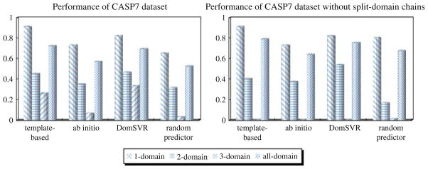
Moreover, we assess both template-based and ab initio predictors on the CASP7 dataset, respectively. Figure 9, respectively, illustrates domain number comparison of such two categories of predictors, our model, and random predictor, with and without split-domain chains. The overall accuracies of domain number prediction for the template-based and ab initio predictors are 72.53 and 56.96%, respectively; while the accuracies are respectively 79.19 and 64.06% if excluding split-domain chains.

Fig. 9.

Performance comparison based on CASP7 dataset. No left-diagonal striped bars are shown in the right graph for template-based, ab initio, and DomSVR predictors, since the prediction accuracies for three-domain chains are zeros

As discussed above, it can be found that our SVR model outperforms other predictors despite of obtaining a lower accuracy for three-domain chains, probably due to the small number of three-domain chains in CASP7 dataset. Actually, more one-domain chains and less chains with two or more domains may make the prediction overestimated. In addition, the small number of chains in CAFASP-4 and CASP7 datasets may also aggravate the trend. Therefore, the evaluation based on a small size of dataset cannot fully reflect the advantages and disadvantaged of these methods. As a result, lager benchmark dataset is more desirable to compare these similar methods in the future.

A case study of domain boundary prediction

In order to illustrate the prediction of domain boundaries directly, protein chain 1qu6A (the same protein discussed as Fig. 3) is taken as a case of domain boundary prediction and shown in Fig. 10. The protein chain has 179 residues and consists of two double-stranded RNA (dsRNA)-binding domains linked by a domain boundary ranging from residue LYS85 to GLY104 (shown in Fig. 10). The protein 1qu6, categorized as kinase PKR (protein kinase RNA-regulated), is an interferon-induced enzyme that plays a key role in the control of viral infections and cellular homeostasis (Nanduri et al. 1998). Protein kinase PKR is activated by a distinct mechanism that involves dsRNA binding in its N-terminal region in an RNA sequence-independent fashion. The structure of dsRNA-binding domain exhibits a dumb-bell shape comprising two tandem linked dsRNA-binding motifs both with an alpha-beta-beta-beta-alpha fold. The structure may reveal a highly conserved RNA-binding site on each dsRNA-binding motif and suggests a novel mode of protein–RNA recognition. The central linker between the two dsRNA-binding motifs is highly flexible, which may enable the two motifs to wrap around the RNA duplex for cooperative and high-affinity binding and advance the overall change of PKR conformation and its activation (Nanduri et al. 1998). The domain boundary prediction for this protein chain is demonstrated in Fig. 10. In this case, our approach predicted the domain boundary actually but a little extension to several residues, ranging from residue VAL77 to residue THR120.

Fig. 10.

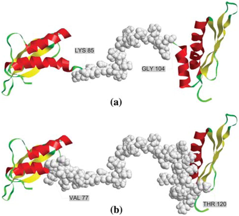
Comparison of natural versus predicted domain boundaries for protein chain 1qu6_A. The domain boundary (true or predicted) is shown as space filling grey spheres. a True domain boundary for protein chain1qu6A, b Predicted domain boundary for protein chain1qu6A

Conclusions

In this paper, we addressed the problem of domain boundaries prediction from sequence information alone. Amino acid residue profiles were taken from AAindex database using PCA technique to extract necessary physicochemical properties. The profiles were then used to train and test our predictor by the form of input vectors. As a result, our method achieves a sensitivity of 36.5% and a specificity of 80.8%. Our method is also evaluated on two datasets: the CAFASP-4 dataset and the CASP7 benchmark dataset. On the CAFASP-4 test dataset, our method performs better than the template-based method InterProScan and comparably to all other template-based methods with respect to specificities. Moreover, our method performs significantly better than all other ab initio methods for domain boundary prediction. On the CASP7 test dataset, our method is able to outperform all the other ab initio methods for two-domain protein chains and slightly worse than some other methods for one-domain protein chains. However, the overall accuracy of our model is the best. It should be noted that the purpose of the comparison is just to estimate the current state-of-the-art of domain boundary prediction instead of ranking these methods, because predictors used different scales of protein set from the CA-FASP-4 and CASP7 datasets to evaluate themselves.

In general, we are not only interested in the overall performance of domain boundary prediction, but also interested in how the prediction accuracy varies across different protein classes by CATH and SCOP architectures. Three hundred and fifty-four protein chains representing all major classes from CATH and SCOP have been chosen for training and testing our method. Mainly beta proteins and fewer SS proteins achieve better prediction compared to other proteins when classifying by CATH. When being classified by SCOP, small proteins show the best sensitivities although containing six protein chains. However, all beta proteins and alpha + beta proteins achieve the second best sensitivities and accuracies. PrinComp1, having strong correlation to inter-residue contact energy property, is the one that the predictor achieves the most reliable results from. The model also achieves very accurate predictions from PrinComp2, PrinComp3, and Prin-Comp4, but the number of correctly predicted domain boundary residues from them is smaller than the model gets from PrinComp1.

The DomSVR algorithm described in this work gives good results for most of proteins in our dataset taken from PDB database. The successful application of SVR approach in this study suggests that SVR can accurately describe the relationship between primary sequence and domain boundaries using amino acid information alone. The predicted domain boundaries can be used for classification of proteins and understanding the evolutions, structures and functions of proteins, which motivate us to improve the algorithm and apply it to other protein chains. In future work, we expect that the improved version of our predictor can test more protein chains and reevaluate the chains that have already been tested with our current predictor.

References

- Altschul SF, Madden TL, Schaffer AA, Zhang J, Zhang Z, Miller W, Lipman DJ. Gapped BLAST and PSI-BLAST: a new generation of protein database search programs. Nucleic Acids Res. 1997;25:3389–3402. doi: 10.1093/nar/25.17.3389. [DOI] [PMC free article] [PubMed] [Google Scholar]
- Baldi P, Brunak S, Chauvin Y, Andersen CA, Nielsen H. Assessing the accuracy of prediction algorithms for classification: an overview. Bioinformatics. 2000;16:412–424. doi: 10.1093/bioinformatics/16.5.412. [DOI] [PubMed] [Google Scholar]
- Bryson K, McGuffin LJ, Marsden RL, Ward JJ, Sodhi JS, Jones DT. Protein structure prediction servers at University College London. Nucleic Acids Res. 2005;33:w36–w38. doi: 10.1093/nar/gki410. [DOI] [PMC free article] [PubMed] [Google Scholar]
- Chen P, Wang B, Wong HS, Huang DS. Prediction of protein B-factors using multi-class bounded SVM. Protein Pept Lett. 2007;14(2):185–190. doi: 10.2174/092986607779816078. [DOI] [PubMed] [Google Scholar]
- Cheng J, Sweredoski MJ, Baldi P. DOMpro: protein domain prediction using profiles, secondary structure, relative solvent accessibility, and recursive neural networks. Data Min Knowl Discov. 2006;13:1–10. [Google Scholar]
- Chivian D, Kim DE, Malmstrom L, Bradley P, Robertson T, Murphy P, Strauss CE, Bonneau R, Rohl CA, Baker D. Automated prediction of CASP-5 structures using the Robetta server. Proteins. 2003;53(S6):524–533. doi: 10.1002/prot.10529. [DOI] [PubMed] [Google Scholar]
- Copley RR, Doerksa T, Letunica I, Borka P. Protein domain analysis in the era of complete genomes. FEBS Lett. 2002;513:129–134. doi: 10.1016/s0014-5793(01)03289-6. [DOI] [PubMed] [Google Scholar]
- Dovidchenko NV, Lobanov MY, Galzitskaya OV. Prediction of number and position of domain boundaries in multi-domain proteins by use of amino acid sequence alone. Curr Protein Pept Sci. 2007;8(2):189–195. doi: 10.2174/138920307780363460. [DOI] [PubMed] [Google Scholar]
- Drucker H, Burges CJC, Kaufman L, Smola AJ, Vapnik V. Support vector regression machines. Proceedings of the NIPS. 1996:155–161. [Google Scholar]
- Dumontier M, Feldman R, Yao HJ, Hogue CWV. Armadillo: doamin boundary prediction by amino acid composition. J Mol Biol. 2005;350:1061–1073. doi: 10.1016/j.jmb.2005.05.037. [DOI] [PubMed] [Google Scholar]
- Edelman GM. Antibody structure and molecular immunology. Science. 1973;180:830–840. doi: 10.1126/science.180.4088.830. [DOI] [PubMed] [Google Scholar]
- Fukuchi S, Nishikawa K. Protein surface amino acid compositions distinctively differ between thermophilic and mesophilic bacteria. J Mol Biol. 2001;309:835–843. doi: 10.1006/jmbi.2001.4718. [DOI] [PubMed] [Google Scholar]
- Galzitskaya OV, Melnik BS. Prediction of protein domain boundaries from sequence alone. Protein Sci. 2003;12:696–701. doi: 10.1110/ps.0233103. [DOI] [PMC free article] [PubMed] [Google Scholar]
- George RA, Heringa J. Protein domain identification and improved sequence similarity searching using PSI-BLAST. Proteins: Struct Funct Gen. 2002;48:672–681. doi: 10.1002/prot.10175. [DOI] [PubMed] [Google Scholar]
- George RA, Heringa J. SNAPDRAGON: a new method to predict protein structural domain boundaries from sequence data. J Mol Biol. 2002;316:839–851. doi: 10.1006/jmbi.2001.5387. [DOI] [PubMed] [Google Scholar]
- Gewehr JE, Zimmer R. SSEP-Domain: protein domain prediction by alignment of secondary structure elements and profiles. Bioinformatics. 2006;22:181–187. doi: 10.1093/bioinformatics/bti751. [DOI] [PubMed] [Google Scholar]
- Goodall C. Modern methods of data analysis. Sage Publications; Newbury Park, CA: 1990. [Google Scholar]
- Gunn SR. Support vector machines for classification and regression. Faculty of Engineering and Applied Science, University of Southampton; 1998. [Google Scholar]
- Heger A, Holm L. Exhaustive enumeration of protein domain families. J Mol Biol. 2003;328:749–767. doi: 10.1016/s0022-2836(03)00269-9. [DOI] [PubMed] [Google Scholar]
- Jolliffe IT. Principal component analysis. Springer; NY: 2002. [Google Scholar]
- Kawashima S, Pokarowski P, Pokarowska M, Kolinski A, Katayama T, Kanehisa M. AAindex: amino acid index database, progress report. Nucleic Acids Res. 2008;36:D202–D205. doi: 10.1093/nar/gkm998. [DOI] [PMC free article] [PubMed] [Google Scholar]
- Levitt M, Chothia C. Structural patterns in globular proteins. Nature. 1976;261:552–558. doi: 10.1038/261552a0. [DOI] [PubMed] [Google Scholar]
- Lexa M, Valle G. PRIMEX: rapid identification of oligonucleotide matches in whole genomes. Bioinformatics. 2003;19:2486–2488. doi: 10.1093/bioinformatics/btg350. [DOI] [PubMed] [Google Scholar]
- Linding R, Russell RB, Neduva V, Gibson TJ. GlobPlot: exploring protein sequences for globularity and disorder. Nucleic Acids Res. 2003;31:3701–3708. doi: 10.1093/nar/gkg519. [DOI] [PMC free article] [PubMed] [Google Scholar]
- Liu J, Rost B. Sequence-based prediction of protein domains. Nucleic Acids Res. 2004;32:3522–3530. doi: 10.1093/nar/gkh684. [DOI] [PMC free article] [PubMed] [Google Scholar]
- Marchler-Bauer A, Anderson JB, Derbyshire MK, DeWeese-Scott C. CDD: a conserved domain database for interactive domain family analysis. Nucleic Acids Res. 2007;35:D237–240. doi: 10.1093/nar/gkl951. [DOI] [PMC free article] [PubMed] [Google Scholar]
- Marsden RL, McGuffin LJ, Jones DT. Rapid protein domain assignment from amino acid sequence using predicted secondary structure. Protein Sci. 2002;11:2814–2824. doi: 10.1110/ps.0209902. [DOI] [PMC free article] [PubMed] [Google Scholar]
- Miyazawa S, Jernigan RL. Self-consistent estimation of inter-residue protein contact energies based on an equilibrium mixture approximation of residues. Proteins. 1999;34:49–68. doi: 10.1002/(sici)1097-0134(19990101)34:1<49::aid-prot5>3.0.co;2-l. [DOI] [PubMed] [Google Scholar]
- Munoz V, Serrano L. Intrinsic secondary structure propensities of the amino acids, using statistical phi–psi matrices: comparison with experimental scale. Proteins. 1994;20:301–311. doi: 10.1002/prot.340200403. [DOI] [PubMed] [Google Scholar]
- Nagarajan N, Yona G. Automatic prediction of protein domains from sequence information using a hybrid learning system. Bioinformatics. 2004;20:1335–1360. doi: 10.1093/bioinformatics/bth086. [DOI] [PubMed] [Google Scholar]
- Nanduri S, Carpick BW, Yang Y, Williams BR, Qin J. Structure of the double-stranded RNA-binding domain of the protein kinase PKR reveals the molecular basis of its dsRNA-mediated activation. EMBO J. 1998;17:5458–5465. doi: 10.1093/emboj/17.18.5458. [DOI] [PMC free article] [PubMed] [Google Scholar]
- Orengo CA, Michie AD, Jones DT, Swindells MB, Thornton JM. CATH: a hierarchic classification of protein domain structures. Structure. 1997;5:1093–1108. doi: 10.1016/s0969-2126(97)00260-8. [DOI] [PubMed] [Google Scholar]
- Porter RR. Structural studies of immunoglobulins. Science. 1973;180:713–716. doi: 10.1126/science.180.4087.713. [DOI] [PubMed] [Google Scholar]
- Rackovsky S, Scheraga HA. Differential geometry and polymer conformation. 4. Conformational and nucleation properties of individual amino acids. Macromolecules. 1982;15:1340–1346. [Google Scholar]
- Saini HK, Fischer D. Meta-DP: domain prediction meta server. Bioinformatics. 2005;21:2917–2920. doi: 10.1093/bioinformatics/bti445. [DOI] [PubMed] [Google Scholar]
- Sikder AR, Zomaya AY. Improving the performance of DomainDiscovery of protein domain boundary assignment using inter-domain linker index. BMC Bioinform. 2006;7:S6. doi: 10.1186/1471-2105-7-S5-S6. [DOI] [PMC free article] [PubMed] [Google Scholar]
- Sim J, Kim SY, Lee J. PRODO: prediction of protein domain boundaries using neural networks. Proteins. 2005;59:627–632. doi: 10.1002/prot.20442. [DOI] [PubMed] [Google Scholar]
- Suyama M, Ohara O. DomCut: prediction of inter-domain linker regions in amino acid sequences. Bioinformatics. 2003;19:673–674. doi: 10.1093/bioinformatics/btg031. [DOI] [PubMed] [Google Scholar]
- von Ohsen N, Sommer I, Zimmer R, Lengauer T. Arby: automatic protein structure prediction using profile-profile alignment and confidence measures. Bioinformatics. 2004;20:2228–2235. doi: 10.1093/bioinformatics/bth232. [DOI] [PubMed] [Google Scholar]
- Wetlaufer DB. Nucleation, rapid folding, and globular intrachain regions in proteins. Proc Natl Acad Sci USA. 1973;70:697–701. doi: 10.1073/pnas.70.3.697. [DOI] [PMC free article] [PubMed] [Google Scholar]
- Ye L, Liu T, Wu Z, Zhou R. Sequence-based protein domain boundary prediction using BP neural network with various property profiles. Proteins: Struct Funct Bioinform. 2007;71:300–307. doi: 10.1002/prot.21745. [DOI] [PubMed] [Google Scholar]
- Yoo PD, Sikder AR, Zhou BB, Zomaya AY. Improved general regression network for protein domain boundary prediction. BMC Bioinform. 2008;9:S12. doi: 10.1186/1471-2105-9-S1-S12. [DOI] [PMC free article] [PubMed] [Google Scholar]
- Zdobnov EM, Apweiler R. InterProScan-an integration platform for the signature-recognition methods in InterPro. Bioinformatics. 2001;17:847–848. doi: 10.1093/bioinformatics/17.9.847. [DOI] [PubMed] [Google Scholar]
- Zhou Y, Vitkup D, Karplus M. Native proteins are surface-molten solids: application of the Lindemann criterion for the solid versus liquid state. J Mol Biol. 1999;285:1371–1375. doi: 10.1006/jmbi.1998.2374. [DOI] [PubMed] [Google Scholar]