Zone Model Predictive Control: A Strategy to Minimize Hyper- and Hypoglycemic Events

Abstract

Background

Development of an artificial pancreas based on an automatic closed-loop algorithm that uses a subcutaneous insulin pump and continuous glucose sensor is a goal for biomedical engineering research. However, closing the loop for the artificial pancreas still presents many challenges, including model identification and design of a control algorithm that will keep the type 1 diabetes mellitus subject in normoglycemia for the longest duration and under maximal safety considerations.

Method

An artificial pancreatic β-cell based on zone model predictive control (zone-MPC) that is tuned automatically has been evaluated on the University of Virginia/University of Padova Food and Drug Administration-accepted metabolic simulator. Zone-MPC is applied when a fixed set point is not defined and the control variable objective can be expressed as a zone. Because euglycemia is usually defined as a range, zone-MPC is a natural control strategy for the artificial pancreatic β-cell.

Clinical data usually include discrete information about insulin delivery and meals, which can be used to generate personalized models. It is argued that mapping clinical insulin administration and meal history through two different second-order transfer functions improves the identification accuracy of these models. Moreover, using mapped insulin as an additional state in zone-MPC enriches information about past control moves, thereby reducing the probability of overdosing. In this study, zone-MPC is tested in three different modes using unannounced and announced meals at their nominal value and with 40% uncertainty. Ten adult in silico subjects were evaluated following a scenario of mixed meals with 75, 75, and 50 grams of carbohydrates (CHOs) consumed at 7 am, 1 pm, and 8 pm, respectively. Zone-MPC results are compared to those of the “optimal” open-loop preadjusted treatment.

Results

Zone-MPC succeeds in maintaining glycemic responses closer to euglycemia compared to the “optimal” open-loop treatment in te three different modes with and without meal announcement. In the face of meal uncertainty, announced zone-MPC presented only marginally improved results over unannounced zone-MPC. When considering user error in CHO estimation and the need to interact with the system, unannounced zone-MPC is an appealing alternative.

Conclusions

Zone-MPC reduces the variability of control moves over fixed set point control without the need to detune the controller. This strategy gives zone-MPC the ability to act quickly when needed and reduce unnecessary control moves in the euglycemic range.

Introduction

Type 1 diabetes mellitus (T1DM) is characterized by the loss of endogenous secretion of insulin from the pancreatic β-cell that is crucial to maintaining euglycemia and, without proper treatment of exogenous insulin injections, causes life-threatening hyperglycemia and keto-acidosis. Because of the lack of insulin secretion, people with T1DM lose their ability to regulate their glycemic levels and suffer from long periods of hyper-glycemia without proper insulin management.

Establishing a near normoglycemia control requires a careful balance among the person’s daily activities, diet, and insulin administration. However, this is not an easy task, and frequent blood glucose measurements must be taken (pre- and postprandial as well as before bedtime) in order to calculate insulin doses or corrective action. Basal–bolus insulin treatment or intense insulin treatment can be administered as multiple daily injections (MDI) or via an insulin pump.¹Different insulin schedules are suggested for MDI therapy based on insulin type/duration of action, daily schedule of the patient, and other medical conditions. Initial doses are calculated based on body weight and are divided into basal and bolus elements. However, because insulin requirements differ throughout the day, and from day to day, this initial setting needs to be fine-tuned to prevent insulin overdosing, which will result in hypoglycemia, or underdosing, which will result in hyperglycemia.¹

The quest for the development of artificial pancreatic β-cells started nearly 4 decades ago. These devices can be described as external or internal closed-loop systems that use continuous glucose measurements to manipulate insulin administration, and therefore compensate for the loss of natural abilities of glucoregulation of people with T1DM. Early attempts to generate an external artificial pancreatic β-cell were undertaken^2,3using both intravenous blood glucose measurements and intravenous insulin administration. Clemens and colleagues⁴used a clamping algorithm with the Biostator glucose-controlled insulin-infusion system and tested it in both animals and humans. Later Steil and collaborators⁵used proportional integral derivative control for insulin administration.

In recent years, model predictive control (MPC) has been shown to be a promising direction for an artificial pancreas control algorithm.⁶Model predictive control is an optimal control algorithm that has been used in the chemical process industries over the last 4 decades.⁷It is based on a computer control algorithm that uses an explicit process model to optimize future process response by manipulating future control moves (CM). The MPC concept was developed in the early 1970s and was referred to as identification and control⁸or as dynamic matrix control by engineers from the Shell Company.⁹Although MPC was originally implemented in petroleum refineries and power plants, it can be found these days in a wide variety of application areas, including aerospace, food, automotive, and chemical applications.¹⁰Among the reasons for the popularity of MPC are its handling of constraints, it accommodation of nonlinearities, and its ability to formulate unique performance criteria.

Model predictive control optimizes every control cycle with a cost function that includes P future process instants, known as prediction horizon, and M future CM, the control horizon. In each cycle, optimization is repeated using updated process data. However, only the first CM of each optimized sequence is implemented in the process. Process input constraints are included directly such that the optimum solution prevents future constraint violation.

Equation (1) describes a typical objective function used in the MPC format engaging three terms¹⁰: a future output trajectory (y_{k + j}) deviation from desired output trajectory (y^r_{k + j}) over a prediction horizon P; a future input (u_{k + j}) deviation from nominal value u_sover control horizon M; and control move increments (Δu_{k + j}) over control horizon M.

$$\begin{array}{l}J\left(\underset{-}{u}\right)={\displaystyle \sum _{j=1}^P\Vert \left({\mathbf{y}}_{k+j}-{\mathbf{y}}_{k+j}^r\right)\Vert }{\mathbf{Q}}_j+{\displaystyle \sum _{j=0}^{M-1}\Vert \left({\mathbf{u}}_{k+j}-u_s\right)\Vert {\mathbf{R}}_j+\Vert \Delta {\mathbf{u}}_{k+j}\Vert }{\mathbf{S}}_j\\ s.t.\\ {\mathbf{x}}_{k+j}=f\left({\mathbf{x}}_{k+j-1},{\mathbf{u}}_{k+j-1}\right)\forall j=1,P\\ {\mathbf{y}}_{k+j}=g\left({\mathbf{x}}_{k+j},{\mathbf{u}}_{k+j}\right)\forall j=1,P\\ u_{\min }\le {\mathbf{u}}_{k+j}\le u_{\max }\forall j=1,M\\ \Delta u_{low}\le \Delta {\mathbf{u}}_{k+j}\le \Delta u_{up}\forall j=1,M\end{array}$$ (1)

The relative share of each of the three components of the objective function is managed by the time-dependent weight matrices Q, S, and R. Optimization is conducted under model constraints (x_{k + j} are model state variables), upon constraints on maximum and minimum nominal input values (u_minand u_max), and on minimum and maximum CM increments (Δu_low and Δu_up). The solution of optimization using the objective function described by Equation (1) for a single control variable is the vector u ∈ R^M.

Advantages of MPC in coping with large time delays and constraints were tested in recent years both in simulation¹¹ and in clinical studies^12,13 as a control strategy for the artificial pancreatic β-cell. Model predictive control is based on recursively repeated open-loop optimizations that minimize a cost function by using model-based predictions. Hovorka and colleagues¹⁴ used a nonlinear model as the core of their MPC, and the controller showed good results with a clinical subject using intravenous glucose measurements and a subcutaneous insulin pump. However, in this study, manual insulin boluses are given for meals and the controller is engaged after the postprandial peak, leaving the feedback control only a minor role in restoring glycemia. Kovatchev and collaborators¹⁵ introduced the control-to-range concept, which combines a predefined basal rate and boluses with a closed-loop algorithm. The algorithm attempts to maximize the time in a predefined range by adjusting controller parameters instead of including the predefined range as an integral component of the cost function. Hovorka and colleagues¹² have published promising results in vivo that described regulation of nocturnal hypoglycemia in children. Ellingsen and associates¹⁶ reported on insulin-on-board (IOB)-MPC, which uses IOB (the residual insulin concentration from a previous insulin administration) as a safety constraint; the IOB-MPC showed relatively robust results in silico.

This work presents an artificial pancreatic β-cell based on zone-MPC that uses mapped-input data and is adjusted automatically by linear difference personalized models. Controlling to a target zone is applied, in general, to controlled systems that lack a specific set point with the controller goal to keep the controlled variables (CV) in a predefined zone. Controlling to a target zone is highly suitable as an artificial pancreatic β-cell because of the absence of a natural glycemic set point rather than of a euglycemic zone. Moreover, an inherent benefit of control to zone as demonstrated by zone-MPC is limiting pump actuation/activity in a way that if glucose levels are within the zone, no extra correction shall be suggested. This feature of this control strategy is highly important in lowering power consumption of the handheld device.

Methods

Autoregression with Exogenous Input

The Zone-MPC model is based on an ARX model.^17,18 The ARX model that serves as the basis for zone-MPC is chosen from a pool of ARX model candidates that differ by the number of past data points utilized (the ARX order). The different ARX models are scored by their prediction abilities over a fixed horizon, and the ARX model that scores the higher prediction R², Equation (2), over a fixed horizon is then estimated again to improve its prediction abilities.

Equation (2) presents the R² index, where y ∈ R^N is a vector of collected data points, ȳ¯ is the mean of collected data points, and ŷ^ ∈ R^N is the predicted value.

$$R^2=1-\frac{{\displaystyle \sum _{k=1}^n{\left({\mathbf{y}}_k-{\widehat{\mathbf{y}}}_k\right)}^2}}{{\displaystyle \sum _{k=1}^n{\left({\mathbf{y}}_k-\overline{y}\right)}^2}}$$ (2)

The R² index approaches 1 for perfect model predictions and 0 for models that do not predict better than a constant mean value.

Autoregression with exogenous input equations use past input/output discrete records to generate a future discrete prediction. For example, Equation (3) describes the connection between predicted output y^ at instant k and past p and q output and input records, respectively.

$$\begin{array}{l}{\widehat{\mathbf{y}}}_k={\alpha }_{\text{1}}{\mathbf{y}}_{k-1}+\dots +{\alpha }_p{\mathbf{y}}_{k-p}+{\beta }_{\text{1}}{\mathbf{u}}_{k-1}+\dots +{\beta }_q{\mathbf{u}}_{k-q}\\ {\widehat{\mathbf{y}}}_k=\varphi ·{\theta }^T\\ \text{\hspace{0.17em}\hspace{0.17em}\hspace{0.17em}\hspace{0.17em}\hspace{0.17em}\hspace{0.17em}\hspace{0.17em}\hspace{0.17em}where}\\ \varphi =[{\mathbf{y}}_{k-1}\dots {\mathbf{y}}_{k-p}{\mathbf{u}}_{k-1}\dots {\mathbf{u}}_{k-q}]\\ \text{\hspace{0.17em}\hspace{0.17em}\hspace{0.17em}\hspace{0.17em}\hspace{0.17em}\hspace{0.17em}\hspace{0.17em}\hspace{0.17em}and}\\ \theta =[{\alpha }_1\dots {\alpha }_p{\beta }_{\text{1}}\dots {\beta }_q]\end{array}$$ (3)

In the presence of observed data y ∈ R^N, where N is the number of collected data points, linear regression can be performed to establish regression vector θ values by minimizing the sum squares of errors between N data records y and predicted values ŷ as it is formulated in Equation (4).

$$\underset{\theta }{\min }\left\{\frac{1}{N}{{\displaystyle \sum _{k=1}^N\left({\mathbf{y}}_k-\varphi \cdot {\theta }^T\right)}}^2\right\}$$ (4)

Regression on past output regressors, [α₁. . . α_p], is defined as autoregression, and the model is referred to as an ARX model.

Determination of ARX model output order, input order, and delay is subject to data validation and complexity considerations. Autoregression with exogenous input model identification is initialized by the researcher’s decision based on reasonable orders and delays. A pool of ARX models is then generated by the different combinatory combinations of orders and delays, and each ARX model is evaluated by its prediction abilities on calibration data and on validation data. Some trade-off can be formulated between model prediction abilities and ARX model complexity, for example, the Akaike information criterion.¹⁸ However, the quality of collected data for identification will eventually govern identification.

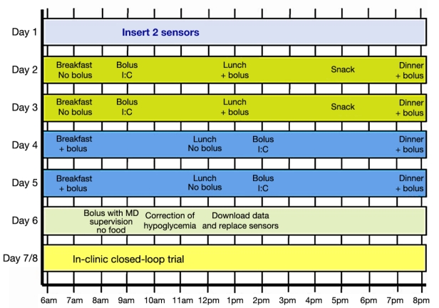
In order to best simulate an in vivo experiment, a data-collecting protocol (Figure 1) introduced by Dassau and collaborators¹⁹ was applied to the Food and Drug Administration (FDA)-accepted University of Virginia (UVa)\University of Padova (Padova) metabolic simulator.²⁰ In the data-collecting protocol, no adjustments to the daily routine were prescribed in day 1. Both days 2 and 3 started at 7 amwith a 25-gram carbohydrate (CHO) breakfast with no insulin bolus, followed by a correction bolus at 9 am; at 1 pma 50-gram CHO lunch was taken together with a correction bolus. A 15-gram CHO snack without a correction bolus was given at 5 pm, and a 75-gram CHO dinner accompanied by an insulin bolus was given at 8 pm. Days 4 and 5 started at 7 amwith a 25-gram CHO breakfast accompanied by an insulin bolus, then a 50-gram lunch was consumed at 12 pm, and an insulin bolus was given at 2 pm. At 8 pma 75-gram CHO dinner accompanied by an insulin bolus was given, and at 10 pman insulin bolus was administered. On the 6^th day the response to a pure bolus from fasting conditions was tested by bolus administration at 9 am.

Figure 1.

Proposed protocol that facilitates the separation of meal and insulin effects on blood glucose.¹⁹

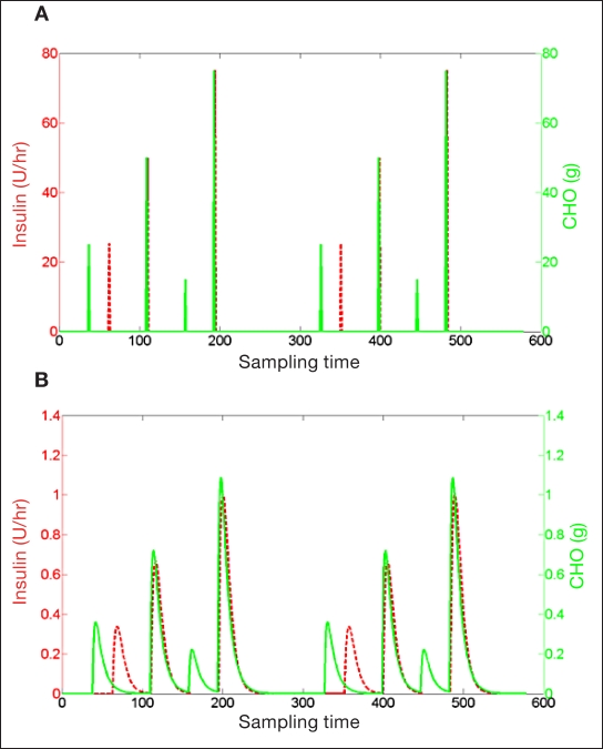
In this work, data of meal and insulin inputs were mapped through second-order transfer functions [Equation (5)] to overcome a major identification problem: a large gain uncertainty was caused by the opposite effects of meal and insulin that are delivered frequently in close time instants. Losing the ability to distinguish between meal and insulin gains can produce poor models for control. However, mapping input data using two different second-order transfer functions (Figure 2) separated and spread input data, providing better terms to regress for the model. Clinical observations and pharmacokinetic/pharmacodynamic data suggest that, on average, the effect of insulin on blood glucose is observed 30 minutes after injection and that the effect of meals on blood glucose is observed after 20 minutes. This a priori knowledge has been used to design the following second-order transfer functions:

Figure 2.

Insulin and meal inputs are mapped through second-order transfer functions and, as a result, are spread and separated. (A) Typical input data collected from T1DM subjects: meals and insulin are assigned as pulses over relatively close discrete time instances. (B) Result of transformed inputs, where each pulse becomes a prolonged time response.

$$\begin{array}{l}{I}_{map}\left(s\right)=\frac{1}{\left(30s+1\right)\left(25s+1\right)}I\left(s\right)\\ M_{map}\left(s\right)=\frac{1}{\left(10s+1\right)\left(45s+1\right)}M\left(s\right)\end{array}$$ (5)

Equation (5) describes transfer functions used to map measured insulin and meal, I and M, respectively, into new states I_mapand M_map. Transfer functions in the Laplace transform²¹ provide the engineer with a powerful method for the analytical solution of differential equations. The Laplace transform is often interpreted as a transformation from the time domain to the frequency domain. The four constants (30, 25, 10, and 45) are in units of minutes.

Horizon Prediction Optimization

The ARX model regressors are normally set by a one step shift of output/input data, such that each prediction at time instant k is evaluated by recorded output/input data up to the time instant k – 1. However, predicted output at instant k is highly correlated to the output measurement at instant k – 1, especially when the sampling time is relatively short. This can lead to ARX models that lose their predictive capabilities.

A novel improvement was suggested to parametric identification of the ARX model as follows: Data are divided into groups of the length of ↓ (N / PH) · PH where N is the number of data points, PH is the prediction horizon, and “↓” is the round down operator. Next, a parametric optimization is carried out in an attempt to find the set of parameters that maximize the prediction in each group. Each group is recursively predicted: the first term of each group is predicted by measured data; then the first term is used to predict the second term in each group; and the predicted terms, first and second, are used to predict the third term. This procedure is repeated for all data points in each group, and the ability to predict all groups is used as a cost function for optimization, Equation (6).

$$\begin{array}{l}\underset{\theta }{\min }\left\{\frac{{\displaystyle \sum _{d=1}^{\downarrow \left(N/PH\right)}{{\displaystyle \sum _{k=\left(d-1\right)\cdot PH+1}^{PH\cdot d}\left({\mathbf{y}}_k-{\mathbf{y}}_{rec,k}\right)}}^2}}{{\displaystyle \sum _{i=1}^N{\left({\mathbf{y}}_i-\overline{y}\right)}^2}}\right\}\\ \text{where}\\ {\mathbf{y}}_{rec}=\{\begin{array}{l}\mathbf{y}\text{\hspace{0.17em}\hspace{0.17em}\hspace{0.17em}\hspace{0.17em}\hspace{0.17em}\hspace{0.17em}\hspace{0.17em}\hspace{0.17em}\hspace{0.17em}\hspace{0.17em}\hspace{0.17em}\hspace{0.17em}\hspace{0.17em}\hspace{0.17em}\hspace{0.17em}if\hspace{0.17em}mod}\left(k,PH\right)=0\\ \varphi \cdot {\theta }^T\text{\hspace{0.17em}\hspace{0.17em}\hspace{0.17em}\hspace{0.17em}\hspace{0.17em}if\hspace{0.17em}mod}\left(k,PH\right)\ne 0\end{array}\\ \varphi =[{\mathbf{y}}_{rec,k-1}\dots {\mathbf{y}}_{rec,k-p}{\mathbf{I}}_{map,k-d_1-1}\dots \\ {\mathbf{I}}_{map,k-d_1-q_1}{\mathbf{M}}_{map,k-d_2-1}\dots {\mathbf{M}}_{map,k-d_2-q_2}]\\ \theta =\left[{\alpha }_1\dots {\alpha }_p{\beta }_1\dots {\beta }_{q_1}{\gamma }_1\dots {\gamma }_{q_2}\right]\end{array}$$ (6)

Horizon prediction optimization [Equation (6)] attempts to minimize normalized sum squares of errors between output recorded data, y, and the recursive prediction in each data group, y_rec. mod(k, PH) is the modulus after the division of · I_map and M_map are mapped insulin and meal data records, respectively. p, q₁, and q₂ are the order of output (glycemia), insulin, and meal, respectively, and d₁ and d₂are insulin and meal delays in sampling time, respectively. α_k, β_k, and γ_kare regressors of glucose, insulin, and meal, respectively.

The following five constraints were applied to the optimization to prevent models from being unstable, having nonphysical gains, or having inverse responses and so that they may be suitable for predictive control:

1. For stability, roots of the following of the characteristic polynomial, z^P– α₁z^P–1– α₂z^P–2... – α₂, are all inside the unit circle.

2. Negative insulin gain requirement, $\frac{{\displaystyle \sum _{i=1}^{q_1}{\beta }_1}}{1-{\displaystyle \sum _{j=1}^{p_1}{\alpha }_j}}<0.$

3. Positive meal gain requirement, $\frac{{\displaystyle \sum _{i=1}^{q_2}{\gamma }_i}}{1-{\displaystyle \sum _{j=1}^p{\alpha }_j}}>0.$

4. No inverse response in insulin, $Sg([{\beta }_1\dots {\beta }_{q_1}])=0$, where $Sg(\overline{x})$ is defined by Equation (7).

No inverse response in meal, $Sg([{\gamma }_1\dots {\gamma }_{q_2}])=0$.

$$Sg\left(\overline{x}\right)=\{\begin{array}{l}\text{0\hspace{0.17em}\hspace{0.17em}\hspace{0.17em}\hspace{0.17em}\hspace{0.17em}\hspace{0.17em}\hspace{0.17em}\hspace{0.17em}\hspace{0.17em}\hspace{0.17em}\hspace{0.17em} For }\overline{\text{x}}\text{ that contains all components on only one side of }\mathbf{0}\\ \text{1\hspace{0.17em}\hspace{0.17em}\hspace{0.17em}\hspace{0.17em}\hspace{0.17em}\hspace{0.17em}\hspace{0.17em}\hspace{0.17em}\hspace{0.17em}For }\overline{\text{x}}\text{ that contains two component from different sides of }\mathbf{0}\end{array}$$ (7)

Equation (7) describes a Boolean function that results in 0 if provided with a vector that has elements on only one side of the origin (i.e., all positive or all negative). The function results in 1 if provided with a vector that has at least two elements from different sides of the origin.

Zone Model Predictive Control

The different MPC algorithms can be classified into four approaches to specify future process response:¹⁰ fixed set point, zone, reference trajectory, and funnel. Using a fixed set point for the future process response can lead to large input adjustments unless settings of the controller are changed in detriment of performance. A zone control is designed to keep the CV in a zone defined by upper and lower boundaries that are usually defined as soft constraints. Some MPC algorithms define a desired response path for CV, called reference trajectory. The reference trajectory usually describes a defined path from the current CV state to a desired set point. The reference trajectory control returns to a fixed set point control when the CV approaches the defined set point. Robust Multivariable Predictive Control Technology (Honeywell Inc., 1995) attempts to keep the CV in a defined zone; however, when the CV is out of the zone, a funnel is defined to bring the CV back into the zone. Kovatchev and colleagues¹⁵ presented the concept of control to range for diabetes that optimizes glucose control to a certain glucose control range. The control-to-range concept is focused on CV performances rather than on controller architecture.

Zone-MPC is applied when the specific set point value of a CV is of low relevancy compared to a zone that is defined by upper and lower boundaries. Moreover, in the presence of noise and model mismatch there is no practical value using a fixed set point. A general description of MPC with output objectives defined as a zone can be found in Maciejowski.²² Our zone-MPC is implemented by defining fixed upper and lower bounds (Figure 3) as soft constraints by letting optimization weights switch between zero and some final values when predicted CVs are in or out of the desired zone, respectively. Predicted residuals are generally defined as the difference between the CV that is out of the desired zone and the nearest bound.

Figure 3.

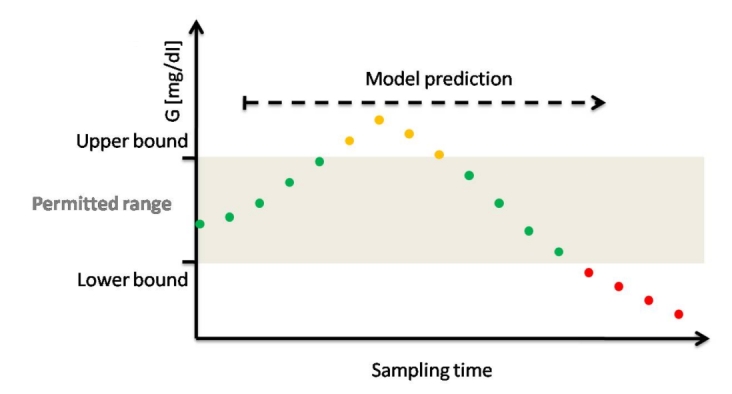
Illustration of zone-MPC in the context of diabetes; zone-MPC is typically divided into three different zones. The permitted range is the control target and is defined by upper and lower bounds. For example, green dots indicate predicted glycemic values in the permitted range. The upper zone represents undesirable high predicted glycemic values, which are represented by orange dots. The lower zone represents undesirable low predicted glycemic values that represent the hypoglycemic zone or a prehypoglycemic protective area that is a low alarm zone. Zone-MPC optimizes predicted glycemia by manipulating insulin CM to stay in the permitted zone under specified constrains.

The core of zone-MPC lies in its cost function formulation. Zone-MPC, like any other form of MPC, predicts the future ŷ ∈ R^P output by an explicit model using past P input/output records and future input u ∈ R^M moves that need to be optimized. However, instead of driving to a specific fixed set point, the optimization attempts to keep or move the predicted outputs into a zone that is defined by upper and lower bounds.

Figure 3 depicts zone-MPC applied to glycemia regulation. Fixed upper and lower glycemic bounds are predefined. Using a linear difference model, glycemic dynamics are predicted and optimization reduces future glycemic excursions from the zone under constraints and weights defined in its cost function.

The zone-MPC cost function used in the presented work is defined as follows:

$$\begin{array}{l}J\left(\underset{¯}{u}\right)={\displaystyle \sum _{j=1}^P\Vert {\mathbf{y}}_{k+j}^{range}\Vert }Q+{\displaystyle \sum _{j=0}^{M-1}\Vert \left({\mathbf{u}}_{k+j}-u_s\right)\Vert }R\\ s.t.\\ {\mathbf{y}}_{k+j}=f\left({\mathbf{y}}_{k+j-1},{\mathbf{u}}_{k+j-1}\right)\forall j=1,P\\ 0\le {\mathbf{u}}_{k\text{+}j}\le u_{\max }\forall j=1,M\end{array}$$ (8)

where Q and R are constant optimization weights on predicted outputs and future inputs, respectively, and y^range is a superposition of all the predicted outputs states that exceed the permitted range:

$${\mathbf{y}}_{k+j}^{range}=\left[{\mathbf{y}}_{k+j}^{lower}{\text{ -lower bound, }\mathbf{y}}_{k+j}^{upper}-\text{\hspace{0.17em}upper bound}\right]$$ (9)

y^lower ∈ R^P collects all predicted points below the lower bound by setting all other predicted values to zero:

$$\begin{array}{l}{\mathbf{y}}^{lower}={\displaystyle \sum _{j=1}^P{\mathbf{y}}_{k+j}\cdot C_j^1}\\ \text{\hspace{0.17em}\hspace{0.17em}\hspace{0.17em}\hspace{0.17em}\hspace{0.17em}\hspace{0.17em}\hspace{0.17em}\hspace{0.17em}\hspace{0.17em}\hspace{0.17em}\hspace{0.17em}\hspace{0.17em}\hspace{0.17em}\hspace{0.17em}\hspace{0.17em}\hspace{0.17em}where}\\ C_j^1=\{\begin{array}{l}1forall{\mathbf{y}}_{k+j}\text{ <\hspace{0.17em}}lowerboundj=1,P\\ 0forall{\mathbf{y}}_{k+j}\ge lowerboundj=1\text{, }P\end{array}\end{array}$$ (10)

y^upper ∈ R^P collects all predicted points above the upper bound by setting all other predicted values to zero:

$$\begin{array}{l}{\text{y}}^{upper}={\displaystyle \sum _{j=1}^p{\mathbf{y}}_{k+j}\cdot C_j^2}\\ \mathrm{where}\\ C_j^2=\{\begin{array}{l}1{\text{for all }\mathbf{y}}_{k+j}\text{ > }upperboundj\text{ = }1,P\\ 0{\text{for all }\mathbf{y}}_{k+j}\le upperboundj\text{ = }1,P\end{array}\end{array}$$ (11)

Future CM are constrained, set by the ability of the insulin pump to deliver a maximum rate of insulin and the inability to deliver negative insulin values. The objective function [Equation (8)] neglects the control move increments component to enable fast control movements.

Input-Transformed Zone-MPC

Second-order input transfer functions described by Equation (5) are used to generate an artificial input memory in zone-MPC schema to prevent insulin overdosing and, as a result, hypoglycemia. In order to avoid overdelivery of insulin, the evaluation of any sequential insulin delivery must take into consideration the past administered insulin against the length of the insulin action. However, a one-state linear difference model with a relative low order uses output (glycemia) as the main source of past administered input (insulin) “memory.” In the face of model mismatch, noise, or change in the subject’s insulin sensitivity, this may result in under- or overdelivery of insulin. This can be mitigated by adding two additional states for mapped insulin and meal inputs.

As discussed earlier, ARX models are identified using mapped inputs. Insulin and meal measurements and transfer functions used for identification can be embedded into one ARX model with one state (glucose) and two inputs (insulin and meal), as illustrated in Equation (12).

$$\begin{array}{l}{\mathbf{G}}_{k+1}={\alpha }_1{\mathbf{G}}_k+\cdots +{\alpha }_p{\mathbf{G}}_{k-p}+{\beta }_{11}{\mathbf{I}}_{k-d_{\text{1}}-1}+\cdots \\ +{\beta }_{1q_1}{\mathbf{I}}_{k-d_1-q_1}+\cdots +{\beta }_{21}{\mathbf{M}}_{k-d_2-1}+\cdots +{\beta }_{2q_2}{\mathbf{M}}_{k-d_2-q_2}\end{array}$$ (12)

where G, I, and M represent glucose blood concentration, insulin administration, and meals, respectively. α_i, β_{1 i}, and β_{2 i} are model coefficients; d₁and d₂are insulin and meal time delays, respectively; and p, q₁, and q₂are orders of glucose, insulin, and meal, respectively.

In order to generate a prediction using Equation (12), we need p past measurements of G and d₁+ q₁and d₂+ q₂past insulin and meal measurements, respectively. However, while G has infinite memory, which is the outcome of the deterministic difference equation, the inputs memory is restricted to past inputs of a restricted order. For example, if delay in insulin, d₁, is equal to two sample times and the order of insulin in the model is equal to three sample times, then the model captured the insulin administration of only five previous sample times. In perfect conditions where there is no model mismatch, no noise, or change in insulin sensitivity, past inputs will be contained into the G dynamics; however, in reality, these conditions are unlikely to be achieved.

An alternative formulation of the model, which provides a full reliable input memory to the system, is described in Equation (13):

$$\begin{array}{cc}{\mathbf{G}}_{k+1}& ={\alpha }_1{\mathbf{G}}_k+\mathrm{...}+{\alpha }_p{\mathbf{G}}_{k-p}+{\beta }_{11}{\mathbf{I}}_{map,k-d_1-1}+\mathrm{...}\\ & +{\beta }_{1q_1}{\mathbf{I}}_{map,k-d_1-q_1}+\mathrm{...}+{\beta }_{21}{\mathbf{M}}_{map,k-d_2-1}\\ & +\mathrm{...}+{\beta }_{2q_2}{\mathbf{M}}_{k-d_2-q_2}\\ {\mathbf{I}}_{map,k+1}& ={\gamma }_1{\mathbf{I}}_{map,k}+{\gamma }_2{\mathbf{I}}_{map,k-1}+{\gamma }_3{\mathbf{I}}_k+{\gamma }_4{\mathbf{I}}_{k-1}\\ {\mathbf{M}}_{map,k+1}& ={\delta }_1{\mathbf{M}}_{map,k}+{\delta }_2{\mathbf{M}}_{map,k-1}+{\delta }_3{\mathbf{M}}_k+{\delta }_4{\mathbf{M}}_{k-1}\end{array}$$ (13)

where I_mapand M_mapare new states representing mapped insulin and meal values, respectively. γ_i and δ_i are new additions to the set of coefficients. These new states represent the insulin and meal after being absorbed into the blood.

Equation (13) describes an improved formulation to Equation (12) that uses mapped insulin and meal inputs (I_mapand M_map, respectively) as additional states (Figure 4). The two new states are evaluated using the two past state records as well as two past input records. Keeping past new state records enables an infinite input memory that is independent of G measurements. The states are updated after each zone-MPC cycle and thereby maintain the influence of all past inputs.

Figure 4.

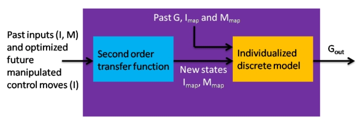
Model prediction structure in zone-MPC includes two parts. First is second-order transfer function that is unvaried over the different subjects. Second is an individualized discrete model that predicts glycemia given mapped input data. The overall prediction is a result of raw data containing past outputs, inputs, and future manipulated CM going through transfer functions and mapped into new states (I_map, M_map) into the individualized discrete model to give the glycemia prediction.

Automatic Controller Tuning

Four main tuning parameters are available for MPC. First, the prediction horizon, P, is a fixed integer indicating the number of prediction samples that will be used by the MPC cost function. P should be on the order of the settling time (ST). Choosing P that is too small will cause the loss of a valuable dynamic response. However, choosing P that is too large will reduce the influence of dynamics over steady state. Second, the control horizon, M, is an integer indicative of the CM that are optimized. A large M will create a sluggish control response; however, choosing M = 1 will cause highly aggressive control. The other two parameters are Q and R, as described earlier. When applying zone-MPC, in addition to the four MPC tuning parameters, zone dimensions can be treated as another tuning variable.

The most dominant dynamic property found to influence zone-MPC tuning was the ST of the ARX model. Settling time is defined as the time it takes for a dynamic system to accomplish 95% of a response to a step input. The prediction horizon P is set to correspond to the individual subject model ST. However, when the ratio between P and M is changed [Equation (8)], then the relative cost between output and input deviations is changed as well.

It should be noted that glucose predictions based on ARX models are limited to approximately 3 hours. Hence, to compensate correctly for prolonged settling times, the weight upon the CM (R) is a function of the ST. In this way we also conserve the balance between weights of the output and input in Equation (8). Moreover, model fitness based on 3 hours of prediction is used as additional penalty upon

$$R=\frac{ST}{{\left({\mathit{FIT}}_{3h}\right)}^{1.5}}$$ (14)

Equation (14) describes the adjusted cost weight upon the CM. The ST is defined by sampling times, and FIT_{3 h} is assumed to have a value greater than 0 and lower than 1 and is calculated by Equation (15):

$${\mathit{FIT}}_{3h}=1-\frac{{\displaystyle \sum _{k=p+1}^{N-PH}{\mathbf{y}}_{3h,k}-{\mathbf{y}}_k}}{{\displaystyle \sum _{j=p+1}^{N-PH}{\mathbf{y}}_j-\overline{y}}}$$ (15)

where y_3h ∈ R^{N − (p + PH)} is a vector containing the collection of ARX model predictions over 3 hours, PH is the number of sampling times contained in 3 hours, and p is the order of autoregressors. N is the total number of data values, y ∈ R ^N is the vector of data values, and ȳ is the mean of data values. Q and M were used as fixed values of 1 and 5, respectively.

Nine control experiments were conducted on 10 in silico adult subjects following a three-meal scenario of 75, 75, and 50 grams of CHO at 7 am, 1 pm, and 8 pm, respectively, using the FDA-accepted UVa\Padova metabolic simulator. In all MPC experiments, the weight upon predicted outputs, Q, is set to 1, while the weight upon future CM, R, is set automatically by Equation (14).

List of Experiments

The zone-MPC model was compared to patient-direct, open-loop control in order to have an objective comparison to other researchers’ work.^23,24Nine experiments were conducted as follows:

Experiment 1: Built-in open-loop preadjusted treatment is applied with nominal meals values.

Experiment 2: Zone-MPC bounds are set between 80 and 140 mg/dl and meals are unannounced.

Experiment 3: Zone-MPC bounds are set between 100 and 120 mg/dl and meals are unannounced.

Experiment 4: Model predictive control with set point at 110 mg/dl and meals are unannounced.

Experiment 5: Zone-MPC bounds are set between 80 and 140 mg/dl and nominal meals are announced.

Experiment 6: Zone-MPC bounds are set between 100 and 120 mg/dl and nominal meals are announced.

Experiment 7: Model predictive control with set point at 110 mg/dl and nominal meals are announced.

Experiment 8: Built-in open-loop preadjusted treatment is tested with meals announced with –40% mismatch with consumed meals value.

Experiment 9: Zone-MPC bounds are set between 80 and 140 mg/dl with meals announced with –40% mismatch with consumed meals value.

Results and Discussion

Unannounced Zone-MPC

Figure 5 depicts the result of a test conducted on subject #5 of the UVa\Padova simulator. In Figure 5, experiments 1 to 4 are represented by gray triangles and red, blue, and black circles, respectively. Figure 5 shows that, the tighter the range of the zone-MPC is, the more variable the CM become. In Figure 5, experiment 1 shows some advantage over MPC experiments on the first meal. This advantage is merely an artifact that resulted from the initial condition (steady state) and the unannounced meal scenario. The controller reacts to the glucose change due to the unannounced meal, compared with the injection treatment where insulin bolus is administered at mealtime. As shown from the dynamic responses, closed-loop control outperforms the manual bolus regimen and provides a better starting point for the following controlled day, as can be seen in the lower glucose value.

Figure 5.

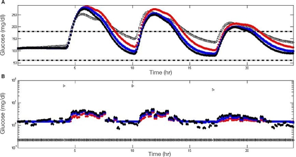
Comparison between experiments 1 to 4 as applied to subject #5 of the UVa\Padova metabolic simulator. Experiments 1 to 4 are represented by gray triangles and red, blue, and black circles, respectively. Glycemic response (A) and insulin administration (B) are depicted. The dashed black line indicates 60 and 180 (mg/dl). Insulin administration is presented in a semilogarithmic scale to include open-loop bolus treatment and controller insulin administrations in a single plot.

Figure 6 presents a population result of experiments 1 to 4, (a) to (d), respectively, on all 10 UVa\Padova subjects. Experiment 1, 2, 3, and 4 mean glucose values are 180, 171, 160, and 155 mg/dl with average standard deviations (SDs) of 27, 22, 23, and 23 mg/dl reaching maximum values of 314, 291, 280, and 274 mg/dl and minimum values of 110, 85, 83, and 76 mg/dl, respectively. Experiment 1 shows the highest mean, SD, and maximum value, which indicate an inferiority of the “optimal” open-loop treatment. For experiments 2 to 4, minimum and maximum values decrease as the range becomes narrower. However, the SD of experiment 2 is the lowest, which implies a decrease in control performance variability among the 10 subjects and indicates higher reliability.

Figure 6.

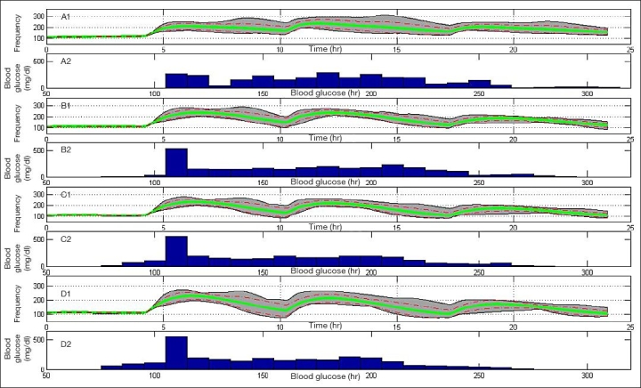
Population result of experiments 1 to 4, (A) to (D), respectively, on 10 UVa\Padova metabolic simulator subjects. Gray area bounds are minimum and maximum points at each given time instant, the green solid line is the mean glycemic response, and dashed red lines are mean glycemic ± SD at each time instant. Glucose distribution for experiments 1 to 4 is presented in the histogram plots.

Announced Zone-MPC

Nominal Meal. Figure 7 shows a comparison among experiments 1, 5, 6, and 7 on subject #5 of the UVa\Padova simulator, which are indicated by gray triangles and red, blue, and black circles, respectively. As shown in Figure 5, the narrower the range of zone-MPC, the more variable the control signal becomes. When announcement of meals is implemented (experiments 5, 6, and 7), zone-MPC presents superior regulation over the open-loop treatment throughout the day by a faster meal disturbance rejection.

Figure 7.

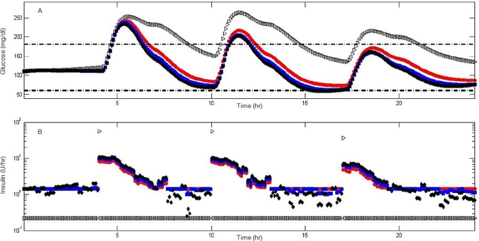
Comparison among experiments 1, 5, 6, and 7 when applied to subject #5 of the metabolic simulator. Experiments 1, 5, 6, and 7 are represented by gray triangles and red, blue, and black circles, respectively. Glycemic response (A) and insulin administration (B) are depicted. Insulin administration is presented in a semilogarithmic scale to include open-loop bolus treatment and controller insulin administrations in a single plot.

Figure 8 presents a population result of experiments 1, 5, 6, and 7, (A) to (D), respectively, on all 10 UVa\Padova subjects. Experiment 1, 5, 6, and 7 mean glucose values are 180, 152, 141, and 136 mg/dl with an average SD of 27, 28, 29, and 29 mg/dl reaching maximum values of 314, 267, 262, and 258 mg/dl and minimum values of 110, 66, 62, and 59 mg/dl, respectively. It can be seen that the result of announced meals is the reduction of mean, maximum, and minimum values. However, reducing minimum values also increase the likelihood of hypoglycemic events, especially for experiment 7. In general, meal announcement introduces additional model uncertainty through the meal gain and dynamics. Therefore, meal announcement will generally reduce glucose levels but may result in a larger variability.

Figure 8.

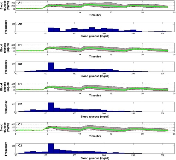
Population result of experiments 1, 5, 6, and 7 on 10 UVa\Padova subjects. Gray area bounds are minimum and maximum points at each given time instant, the green solid line is the mean glycemic response, and dashed red lines are mean glycemic ± SD at each time instant. Glucose distribution for experiments 1, 5, 6, and 7 is presented in the histogram plots.

Forty Percent Meal Uncertainty. Figure 9 describes population responses on the 10 UVa\Padova subjects using experiments 8, 2, and 9 [Figure 9 (A) to (C), respectively]. Experiment 2, 8, and 9 mean glucose values are 171, 205, and 161 mg/dl with an average SD of 22, 36, and 24 mg/dl reaching maximum values of 291, 364, and 274 mg/dl and minimum values of 85, 110, and 85 mg/dl, respectively. Experiment 8 shows the obvious disadvantage of using open-loop treatment in the face of uncertainties. Experiment 8 results in extended hyperglycemia with extreme glucose values over 300 mg/dl. Comparing experiments 2 and 9, advantages of the meal announcement decrease in face of uncertainties, and the two experiments reach similar performance indices.

Figure 9.

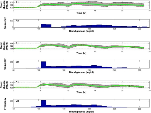
Population result of experiments 2, 8, and 9 on 10 UVa\Padova subjects. Gray area bounds are minimum and maximum points at each given time instant, the green line is the mean glycemic response, and dashed red lines are mean glycemic ± SD at each time instant. Glucose distribution for experiments 2, 8, and 9 is presented in the histogram plots.

Results Summary. Table 1 presents a summary of all UVa/Padova subjects using experiments 1 to 9. Experiment 9 shows the highest time over 180 mg/dl (TO₁₈₀) for all subjects. The single hypoglycemic event occurs with subject #5 during experiment 7. Experiment 7 also presents the lowest time of TO₁₈₀for all subjects.

Table 1.

Summary Results of Time Spent over 180 mg/dl [TO₁₈₀(min)] and Number of Hypoglycemic Events [Hypo_#(–)] for 10 Subjects in All Nine Experiments

Subject #		Exp#1	Exp#2	Exp#3	Exp#4	Exp#5	Exp#6	Exp#7	Exp#8	Exp#9
1	TO180	1107	1074	970	938	1006	947	919	1156	1018
	Hypo#	0	0	0	0	0	0	0	0	0
2	TO180	993	587	412	221	487	189	156	1115	540
	Hypo#	0	0	0	0	0	0	0	0	0
3	TO180	657	486	471	456	455	434	417	730	470
	Hypo#	0	0	0	0	0	0	0	0	0
4	TO180	1140	587	480	466	57	0	0	1147	155
	Hypo#	0	0	0	0	0	0	0	0	0
5	TO180	708	635	538	485	208	171	160	889	405
	Hypo#	0	0	0	0	0	0	1	0	0
6	TO180	1149	766	596	520	635	417	259	1150	711
	Hypo#	0	0	0	0	0	0	0	0	0
7	TO180	413	428	309	291	73	56	58	739	195
	Hypo#	0	0	0	0	0	0	0	0	0
8	TO180	457	855	585	523	612	475	349	1098	743
	Hypo#	0	0	0	0	0	0	0	0	0
9	TO180	153	385	319	269	265	181	120	477	324
	Hypo#	0	0	0	0	0	0	0	0	0
10	TO180	492	596	444	421	233	119	88	885	423
	Hypo#	0	0	0	0	0	0	0	0	0

^aAs noted, Exp#8 (Experiment #8, open-loop with 40%) meal uncertainty shows the highest time over 180 mg/dl in minutes for all 10 subjects. Subject #5 experienced a single hypoglycemic event following experiment 7 (Exp#7). Experiment #7 also presents minimal duration over 180 mg/dl for all subjects.

Conclusions

Zone-MPC was evaluated on the FDA-accepted UVa\Padova metabolic simulator. The control is based on ARX models that were identified in a novel approach by mapping insulin and meal inputs by overdamped second-order transfer functions. Mapped inputs are used as additional state variables in zone-MPC formulation that enables a larger memory for insulin administration. Zone-MPC has shown the ability to handle announced and unannounced meals with meal uncertainties. Zone-MPC showed significant advantages over the “optimal” open-loop treatment. Moreover, zone-MPC reduces control move variability with minimal loss of performance compared to set point control. The ability to attenuate pump activity in the face of noisy CGM has been demonstrated by zone-MPC, which results in safer insulin delivery, as well as minimized power drain on the battery. An enabling step toward a commercial product is that the ability to proceed from CGM measurements directly into a functional controller in a fully automated fashion has been demonstrated. Personalized zone-MPC is a perfect candidate for the fully automated artificial pancreatic β-cell.

Abbreviations

ARX

autoregression with exogenous input

CHO

carbohydrate

CM

control moves

CV

controlled variables

FDA

Food and Drug Administration

IOB

insulin-on-board

MDI

multiple daily injections

MPC

model predictive control

Padova

University of Padova

PH

prediction horizon

ST

settling time

SD

standard deviation

T1DM

type 1 diabetes mellitus

TO₁₈₀

time (min) over 180 mg/dl)

UVa

University of Virginia

References

- 1.Skyler JS. Atlas of diabetes. 3rd ed. Philadelphia: Current Medicine Group LLC; 2005. [Google Scholar]
- 2.Albisser AM, Leibel BS, Ewart TG, Davidovac Z, Botz CK, Zingg W. An artificial endocrine pancreas. Diabetes. 1974;23(5) doi: 10.2337/diab.23.5.389. [DOI] [PubMed] [Google Scholar]
- 3.Pfeiffer EF, Thum C, Clemens AH. The artificial beta cell—a continuous control of blood sugar by external regulation of insulin infusion (glucose controlled insulin infusion system) Horm Metab Res. 1974;6(5):339–342. doi: 10.1055/s-0028-1093841. [DOI] [PubMed] [Google Scholar]
- 4.Clemens A, Hough D, D’Orazio P. Development of the Biostator glucose clamping algorithm. Clin Chem. 1982;28(9):1899–1904. [PubMed] [Google Scholar]
- 5.Steil GM, Panteleon AE, Rebrin K. Closed-loop insulin delivery—the path to physiological glucose control. Adv Drug Deliv Rev. 2004;56(2):125–144. doi: 10.1016/j.addr.2003.08.011. [DOI] [PubMed] [Google Scholar]
- 6.Harvey RA, Youqing W, Grosman B, Percival MW, Bevier W, Finan DA, Zisser H, Seborg DE, Jovanovic L, Doyle FJ, III, Dassau E. Quest for the artificial pancreas: combining technology with treatment. IEEE Eng Med Biol. 2010;29(2):53–62. doi: 10.1109/MEMB.2009.935711. [DOI] [PMC free article] [PubMed] [Google Scholar]
- 7.García CE, Prett MD, Morari M. Model predictive control: theory and practice—a survey. Automatica. 1989;25(3):335–348. [Google Scholar]
- 8.Richalet J, Rault A, Testud JL, Papon J. Algorithmic control of industrial processes. Proceedings of the 4th IFAC Symposium on Identification and System Parameter Estimation; 1976. pp. 1119–1167. [Google Scholar]
- 9.Cutler CR, Ramaker BL. Dynamic matrix control—a computer control algorithm. AIChE national meeting; Houston, TX. 1979. [Google Scholar]
- 10.Qin SJ, Badgwell TA. A survey of industrial model predictive control technology. Control Eng Pract. 2003;11(7):733–64. [Google Scholar]
- 11.Parker RS, Doyle FJ, FJ, Peppas NA. A model-based algorithm for blood glucose control in type I diabetic patients. IEEE Trans Biomed Eng. 1999;46(2):148–157. doi: 10.1109/10.740877. [DOI] [PubMed] [Google Scholar]
- 12.Hovorka R, Allen JM, Elleri D, Chassin LJ, Harris J, Xing D, Craig Kollman, Hovorka T, Larsen AMF, Nodale M, De Palma A, Wilinska ME, Acerini CL, Dunger DB. Manual closed-loop insulin delivery in children and adolescents with type 1 diabetes: a phase 2 randomised crossover trial. Lancet. 2010;375(9716):743–751. doi: 10.1016/S0140-6736(09)61998-X. [DOI] [PubMed] [Google Scholar]
- 13.El-Khatib FH, Russell SJ, Nathan DM, Sutherlin RG, Damiano ER. A bihormonal closed-loop artificial pancreas for type 1 diabetes. Sci Transl Med. 2010;2(27):1–12. doi: 10.1126/scitranslmed.3000619. [DOI] [PMC free article] [PubMed] [Google Scholar]
- 14.Hovorka R, Canonico V, Chassin LJ, Haueter U, Massi-Benedetti M, Federici MO, Pieber TR, Schaller HC, Schaupp L, Vering T, Wilinska ME. Nonlinear model predictive control of glucose concentration in subjects with type 1 diabetes. Physiol Meas. 2004;25(4):905–920. doi: 10.1088/0967-3334/25/4/010. [DOI] [PubMed] [Google Scholar]
- 15.Kovatchev B, Patek S, Dassau E, Doyle FJ, III, Magni L, De Nicolao G, Cobelli C. Control to range for diabetes: functionality and modular architecture. J Diabetes Sci Technol. 2009;3(5):1058–1065. doi: 10.1177/193229680900300509. [DOI] [PMC free article] [PubMed] [Google Scholar]
- 16.Ellingsen C, Dassau E, Zisser H, Grosman B, Percival MW, Jovanoviĉ L, Doyle FJ., III Safety constraints in an artificial pancreatic β-cell: an implementation of model predictive control with insulin on board. J Diabetes Sci Technol. 2009;3(3):536–544. doi: 10.1177/193229680900300319. [DOI] [PMC free article] [PubMed] [Google Scholar]
- 17.Ljung L. System identification toolbox. 6th ed. Natick, MA: The MathWorks, Inc.; 2005. [Google Scholar]
- 18.Lennart L. System identification theory for the user. 2ed ed. Upper Saddle River, NJ: Prentice Hall; 1999. [Google Scholar]
- 19.Dassau E, Zisser H, Grosman B, Bevier W, Percival MW, Jovanoviĉ L, Doyle FJ., Jr Artificial pancreatic β-cell protocol for enhanced model identification. 69th American Diabetes Association Meeting. Vol 59 (Supl1).; New Orleans, LA: Diabetes; 2009. pp. A105–A106. [Google Scholar]
- 20.Kovatchev BP, Breton M, Dalla Man C, Cobelli C. In silico preclinical trials: a proof of concept in closed-loop control of type 1 diabetes. J Diabetes Sci Technol. 2009;3(1):44–55. doi: 10.1177/193229680900300106. [DOI] [PMC free article] [PubMed] [Google Scholar]
- 21.Marlin TE. Process control: designing processes and control systems for dynamic performance. McGraw-Hill, Inc.: 1995. [Google Scholar]
- 22.Maciejowski JM. Predictive control with constraints. Harlow, UK: Prentice-Hall, Pearson Education Limited; 2002. [Google Scholar]
- 23.Clarke WL, Anderson S, Breton M, Patek S, Kashmer L, Kovatchev B. Closed-loop artificial pancreas using subcutaneous glucose sensing and insulin delivery and a model predictive control algorithm: the Virginia experience. J Diabetes Sci Technol. 2009;3(5):1031–1038. doi: 10.1177/193229680900300506. [DOI] [PMC free article] [PubMed] [Google Scholar]
- 24.Lee H, Bequette BW. A closed-loop artificial pancreas based on model predictive control: human-friendly identification and automatic meal disturbance rejection. Biomed Signal Proc Control. 2009;4(4):347–354. [Google Scholar]