A 2D MTF approach to evaluate and guide dynamic imaging developments

Abstract

As the number and complexity of partially sampled dynamic imaging methods continue to increase, reliable strategies to evaluate performance may prove most useful. In the present work, an analytical framework to evaluate given reconstruction methods is presented. A perturbation algorithm allows the proposed evaluation scheme to perform robustly without requiring knowledge about the inner workings of the method being evaluated. A main output of the evaluation process consists of a 2D modulation transfer function (MTF), an easy-to-interpret visual rendering of a method’s ability to capture all combinations of spatial and temporal frequencies. Approaches to evaluate noise properties and artifact content at all spatial and temporal frequencies are also proposed. One fully sampled phantom and three fully sampled cardiac cine datasets were subsampled (R=4 and 8), and reconstructed with the different methods tested here. A hybrid method, which combines the main advantageous features observed in our assessments, was proposed and tested in a cardiac cine application, with acceleration factors of 3.5 and 6.3 (skip factor of 4 and 8, respectively). This approach combines features from methods such as k-t sensitivity-encoding (k-t SENSE), unaliasing by Fourier encoding the overlaps in the temporal dimension-SENSE (UNFOLD-SENSE), generalized autocalibrating partially parallel acquisition (GRAPPA), sensitivity profiles from an array of coils for encoding and reconstruction in parallel (SPACE-RIP), self, hybrid referencing with UNFOLD and GRAPPA (SHRUG) and GRAPPA-enhanced sensitivity maps for SENSE reconstructions (GEYSER).

Introduction

Several clinical applications of MRI involve acquiring a time series of images, to capture dynamic changes within the anatomy of interest. Such dynamic applications include cardiac cine imaging, functional MRI (fMRI), time-resolved contrast-enhanced angiography and perfusion imaging. Partially-sampled methods, whereby only a fraction of a full k-space matrix actually gets acquired, can accelerate the acquisition process and enable valuable improvements such as increased temporal resolution, spatial coverage, spatial resolution and/or contrast. Common methods to achieve this are parallel imaging and partial-Fourier imaging, which can be of great value in both dynamic and non-dynamic applications. However, the presence of a temporal dimension in dynamic applications lends itself to further acceleration strategies and extra imaging speed. Methods specifically designed for dynamic applications include ‘Unaliasing by Fourier encoding the overlaps in the temporal dimension’ (UNFOLD) (1), ‘kt Broad-use Linear Acquisition Speed-up Technique’ (k-t BLAST) (2), ‘Adaptive sensitivity encoding incorporating temporal filtering’ (TSENSE) (3), UNFOLD-SENSE (4), k-t SENSE (2), ‘Patient-adaptive reconstruction and acquisition in dynamic imaging with sensitivity encoding’(PARADISE) (5) ‘Reconstruction of undersampled dynamic images by modeling the motion of object elements’ (6), keyhole (7), x-f choice (8), ‘reduced field-of-view imaging by direct Fourier inversion’ (Noquist) (9), ‘Time-resolve imaging of contrast kinetics’ (TRICKS) (10) and ‘UNFOLD using a temporal subtraction and spectral energy comparison technique’ (T-SUSPECT) (11).

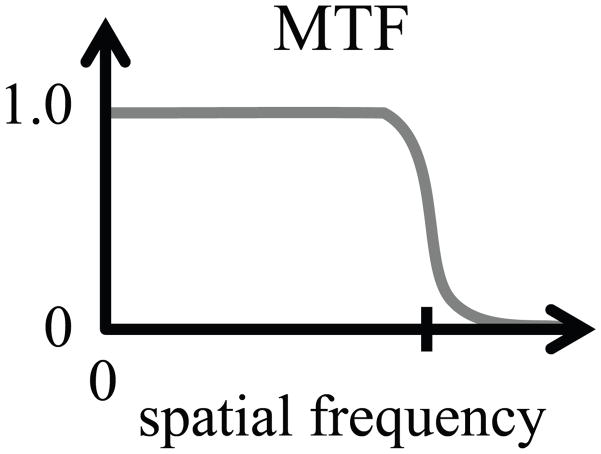
As the variety and complexity of partially sampled dynamic imaging methods continue to increase, understanding how these methods relate and perform becomes increasingly difficult. Modulation transfer functions (MTF) have been used extensively in medical imaging in general, and X-ray imaging in particular, to evaluate the performance of imaging systems. An MTF graphically displays the ability of a given imaging system to correctly capture a range of spatial frequencies. A sharp drop in the MTF marks the resolution limit of a given system, as depicted in Fig. 1 with a tick mark on the spatial frequency axis. In dynamic imaging, both spatial and temporal variations are of interest, and accordingly we propose extending the MTF approach to a 2D plane featuring both spatial and temporal frequency dimensions, labeled k and f, respectively. An ideal dynamic imaging method would be characterized by a homogenous MTF, equal to one across the entire k-f plane.

Figure 1.

An MTF captures the resolving power of a given imaging process, in terms of spatial frequency. In the depiction shown here, a tick mark indicates the resolution limit where a sharp drop can be observed.

Typically, the performance of given dynamic imaging methods might have been measured based on particular examples, such as cardiac results from one or more human subject(s). While very useful, such tests remain anecdotal in nature, as they cannot establish whether the tested method would perform similarly well on different objects and/or subjects, as different combinations of spatial and temporal frequency variations might be present. The primary goal of the present work is to propose a more thorough strategy to evaluate a method’s performance by testing its response to all possible combinations of spatial and temporal frequencies. While the present 2D MTF approach aims at visualizing how well signal gets captured by a given imaging process, noise is another crucial marker of image quality. We further propose a Monte Carlo scheme to evaluate noise properties at all combinations of spatial and temporal frequencies, to complement the signal evaluation from the 2D MTF approach.

The present work is most definitely not aimed at judging or ranking existing dynamic imaging methods, but rather at identifying the main strengths of these methods in a hope that favorable characteristics might prove compatible and give rise to improved hybrid schemes. Our work to date has focused, to a large degree, on testing a number of variations of the k-t SENSE and UNFOLD-SENSE approaches. The power of the clever regularization scheme introduced by Tsao et al. (2), based on low-resolution prior knowledge, is clearly captured by our 2D MTF approach. Strengths of the UNFOLD-SENSE sampling strategy, with larger k-space offsets from frame to frame, are also demonstrated. The merger of these strengths, i.e., the k-t SENSE regularization strategy and the UNFOLD-SENSE encoding scheme, leads to a hybrid approach that performs better than UNFOLD-SENSE at higher acceleration settings and arguably as fast as k-t SENSE, without any of the ‘blind spots’ in temporal frequency that affect k-t SENSE reconstructions and to which UNFOLD-SENSE is mostly immune. This hybrid approach has been tested in a retrospectively gated cardiac cine application, and results are presented here.

Implementing and evaluating all dynamic imaging methods in existence today would prove a very ambitious goal, one that the present manuscript of course cannot come close to achieving. It is hoped however that in time, the introduction of more thorough procedures for evaluating performance will help toward identifying desirable features and combining them into improved hybrid methods, as done here with the development of a (k-t SENSE)-(UNFOLD-SENSE) hybrid.

Our proposed 2D MTF measurement method is described in the Theory section, along with a Monte Carlo algorithm for evaluating noise properties. Following background information about k-t space sampling, the UNFOLD-SENSE and k-t SENSE reconstruction strategies are explained and merged. Still in the Theory section, the use of prior knowledge in several existing dynamic-imaging methods will be described and compared. UNFOLD-SENSE, k-t SENSE and a merged version of the two were evaluated in terms of 2D MTF, noise and artifact properties, based on phantom and in vivo results, as shown in the Results section.

Theory

1. Performance evaluation based on 2D MTF measurements

The image acquisition process can typically be represented as a linear problem of the form

$$\mathbf{K}=\mathbf{F}(\mathbf{E}\mathbf{\rho }+\mathbf{\eta }),$$ [1]

where ρ represents the imaged object (in either x-y-z-t space, k_x-k_y-k_z-f space, or some other hybrid space), η denotes the noise, K is the measured signal, F is an optional filter and E represents the encoding process. The filtering operation refers to cases such as in UNFOLD whereby artifacts are encoded into pre-determined regions of the space encompassed by K, and then removed.

In principle at least, as long as the encoding matrix can be explicitly constructed, the inverse problem can be analytically solved through a matrix inversion and/or an iterative solver. But especially in dynamic imaging, where a time series of images is obtained, the size of the problem described in Eq. 1 may be daunting. Existing accelerated dynamic imaging methods successfully break this reconstruction problem into a large number of smaller and more manageable ones, while introducing prior knowledge and assumptions into the solution.

Assuming for a moment that Eq. 1 could be solved despite its size, a typical approach would be to use a least-squares minimization solution along with a Tikhonov regularization term:

$$\widehat{\mathbf{\rho }}={({\mathbf{E}}^H{\mathbf{F}}^H\mathbf{FE}+\lambda {\mathbf{L}}^H\mathbf{L})}^{-1}{\mathbf{E}}^H{\mathbf{F}}^H\mathbf{K},$$ [2]

where the superscript H represents the adjoint operation, and a Gram matrix L^H L with weight λ is used for regularization purposes. In a case where the ‘truth’ ρ is actually known, combining Eqs 1 and 2 leads to:

$$\begin{array}{l}\widehat{\mathbf{\rho }}={({\mathbf{E}}^H{\mathbf{F}}^H\mathbf{FE}+\lambda {\mathbf{L}}^H\mathbf{L})}^{-1}{\mathbf{E}}^H{\mathbf{F}}^H\mathbf{F}(\mathbf{E}\mathbf{\rho }+\mathbf{\eta })=\mathbf{H}\mathbf{\rho }+\widehat{\mathbf{\eta }};\\ \mathbf{H}={({\mathbf{E}}^H{\mathbf{F}}^H\mathbf{FE}+\lambda {\mathbf{L}}^H\mathbf{L})}^{-1}{\mathbf{E}}^H{\mathbf{F}}^H\mathbf{FE}.\end{array}$$ [3]

The H matrix essentially transforms signal from the actual object to its imaged version. Expressing Eq. 3 in terms of the individual elements of H, one obtains:

$${\widehat{\rho }}_i=H_{ii}{\rho }_i+\sum _{j;i\ne j}{H}_{ij}{\rho }_j+{\widehat{\eta }}_i.$$ [4]

For an ideal imaging system, where the image of an object is identical to the object itself, the H_ii and H_ij coefficients would be equal to, respectively, ones and zeros. In a case where ρ is expressed in the spatial-temporal frequency domain (kx-ky-f), the H_ii coefficients in Eq. 4 correspond to the MTF we are seeking to build, as they represent the ability of a given imaging system to capture all combinations of spatial and temporal frequencies. Non-zero H_ij terms, on the other hand, represent artifacts introduced by the imaging system, whereby signal that belongs to a given combination of spatial and temporal frequencies gets erroneously mapped to a different frequency location.

As previously stated, due to the large size of the problem expressed in Eq. 1, the matrix H as expressed in Eq. 3 may not be explicitly known. Instead, we propose a perturbation approach to evaluate the MTF associated with a given imaging process. As can be seen from Eq. 4, for any given value of i, the desired MTF entry H_ii would act as a slope in a plot of ρ̂_i vs ρ_i. A small perturbation P_i,p is added to the ‘truth’ ρ_i, where the subscript p denotes the index of the perturbation. This new ‘truth’, with i^th entry ρ_i,p, is subsampled and reconstructed to yield a new imaged version, with i^th entry ρ̂_i,p. After adding successively several different amounts of perturbation, linear regression is performed on ρ_i,p and ρ̂_i,p:

$${\widehat{\rho }}_{i,p}=B_i({\rho }_i+P_{i,p})+A_i=B_i{\rho }_{i,p}+A_i,$$ [5]

where A_i and B_i are fit coefficients. The perturbation should be kept very small as significant changes to the ‘truth’ could artificially render the prior knowledge and assumptions used by various methods inaccurate, and unfairly affect their measured performance. Round-off errors appear to be the only factor limiting how small the perturbations can be made. The fit slope B_i, like H_ii in Eq. 4, represents how well signals get transferred from object (input) to image (output). The intercept A_i, on the other hand, reveals signal erroneously reconstructed at a given frequency, whose presence and intensity in the output is independent of whether we perturb this frequency at the input.

The variables in Eq. 5 represent individual elements from corresponding arrays described as ρ̂(k_x, k_y, f, p), A(k_x,k_y,f), ρ(k_x, k_y, f, p) and B(k_x,k_y,f), respectively. In 2D imaging cases where the sampling is Cartesian along k_x, no variations in MTF are expected along this direction and a sum is performed, leaving only a 2D MTF with k_y and f coordinates. After summation and proper scaling, the fit coefficients B(k_x,k_y,f) and A(k_x,k_y,f) give rise to the 2D MTF and signal to artifact measures used in the present work:

$${\mathbf{T}}_{\text{MTF}}(ky,f)=\sqrt{\frac{{\displaystyle \sum _x}\mid \mathbf{B}(x,ky,f){\mid }^2}{N_x}}$$ [6]

$${\mathbf{T}}_{\rho /A}(ky,f)={\mathbf{T}}_{\text{MTF}}(ky,f)\sqrt{\frac{{\displaystyle \sum _x}\mid \mathbf{\rho }(x,ky,f){\mid }^2}{{\displaystyle \sum _x}\mid \mathbf{A}(x,ky,f){\mid }^2}},$$ [7]

2. Performance evaluation based on noise measurements

Monte Carlo methods have been extensively applied to assess statistical properties of stochastic processes, and involve using random numbers through several simulated iterations. Such approach can be used here to capture the noise properties of a given algorithm (12), without the need to explicitly obtain the H matrix in Eq. 3. For each iteration complex Gaussian distributed random numbers were input in place of the acquired data, for all coils and all time frames. The purely noisy data were undersampled in accordance with the sampling scheme and acceleration factor being probed. The resulting noise datasets were reconstructed using parameters, such as sensitivity maps and regularization information, obtained from the original acquired dataset, giving rise to noisy reconstructed results ρ̂_R where R stands for the acceleration factor. A noise enhancement ratio is obtained by dividing the variance at each spatial and temporal frequency location by the corresponding variance from the R = 1 case(9):

$$\mathbf{N}(ky,f)=\sqrt{\frac{{\displaystyle \sum _x}\mathit{Var}\{{\widehat{\mathbf{\rho }}}_R(x,ky,f)\}}{{\displaystyle \sum _x}\mathit{Var}\{{\widehat{\mathbf{\rho }}}_1(x,ky,f)\}}}.$$ [8]

Because Eq. 8 estimates a ratio, the scaling of the noise being introduced as part of the Monte Carlo approach has no impact on the results, as any non-zero finite scaling would simply cancel out in Eq. 8.

While the 2D MTF and noise measurement algorithms described here are, in principle at least, were aimed at a fairly wide range of dynamic imaging methods, results in the present work were obtained for variants of the k-t SENSE and UNFOLD-SENSE schemes, including a hybrid of the two. Accordingly, the following sections give a quick overview of the main characteristics of these two approaches, focusing especially on characteristics that will prove useful toward interpreting our 2D MTF and noise results.

3. On the sampling of k-t space

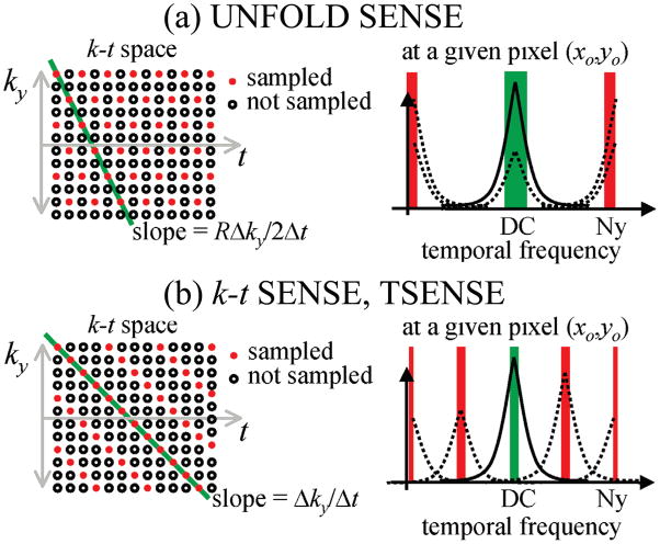
Several dynamic imaging methods involve shifting or rotating the sampling function in k-space from time frame to time frame (13). The rationale for such time-varying acquisition schemes is illustrated in Fig. 2, for an acceleration factor R = 4. In any given image pixel (x_o, y_o), up to 4 components overlap: 3 aliased (dashed lines in Fig. 2) and 1 non-aliased (solid line). Time-varying sampling schemes have the effect of moving some or all of the aliased energy away from the temporal DC region, where most of the non-aliased signal remains (1). The steeper the slope in k-t space, the further the aliased energy gets displaced, although wraparound does occur from −Nyquist to +Nyquist and vice-versa. In Fig. 2, much of the artifact energy (dashed lines) was moved away from the DC region, creating a zone near DC and highlighted in green where the aliasing problem has been considerably simplified. Because much of the non-aliased signal is found near DC, a simplified signal reconstruction problem around DC can lead to considerably improved overall image quality.

Figure 2.

The sampling schemes of UNFOLD-SENSE (a) and k-t SENSE (b) are depicted here. The spectrum for one single (x_o,y_o) pixel in the aliased image is shown on the right, side, for each sampling scheme. The steeper slope typically selected in UNFOLD-SENSE pushes half of all overlapped signals to the Nyquist frequency. In contrast, the gentler slope selected in k-t SENSE evenly distributes the aliased components along the temporal bandwidth. For both methods, their strength comes from reducing the amount of overlap found at DC (frequency bands highlighted in green) and their weakness from the fact that weak non-aliased signal cannot be reliably recovered when overwhelmed with strong aliased signal (frequency bands highlighted in red).

The downside of such time-varying sampling strategies can be appreciated looking at the temporal frequency regions highlighted in red in Fig. 2. The aliased energy displaced from DC must of course appear somewhere else, and weak non-aliased signal is unlikely to be properly recovered when overwhelmed by strong aliased signal. In k-t SENSE, a relatively small slope setting is used in k-t space, i.e., the k-space increment from frame to frame is relatively small (Fig. 2). While the overlap problem near DC (green zone) is almost entirely resolved, several difficult areas are created (red zones). With an acquisition scheme based on variable-density sampling and a steeper slope in k-t space, UNFOLD-SENSE creates only one difficult region (near Nyquist, shown in red), although it only partly solves the aliasing problem near DC. This difference in the preferred slope setting in k-t space gives rise to some of the main differences we noted between the 2D MTF obtained from the two methods.

A great strength of such methods with a time-varying sampling function is that the DC region (green band, Fig. 2) can be easily obtained once most or all aliased components have been cleared away. On the other hand, a typical weakness is the difficulty to recover weak non-aliased signals wherever they are overwhelmed by intense aliased signals (red bands, Fig. 2). For display purposes and if so desired, 2D y-f plots at a given x₀ location, of the type used in (2), could be used just as well as the 1D f plots at a given (x_o,y_o) location used in Fig. 2 and in (1).

4. UNFOLD-SENSE and k-t SENSE reconstruction methods

UNFOLD-SENSE

The UNFOLD-SENSE reconstruction equation is given by (14)

$$\widehat{\rho }(x,f)=O_l\left\{F_{+\text{DC}}\right\{K_{\mathbf{\gamma }}(k,f)\left\}\right\}+O_r\left\{F_{-\text{alias}}\right\{K_{\mathbf{\gamma }}(k,f)\left\}\right\},$$ [9]

Where K_γ is the signal from coil number γ, O_l is a parallel imaging reconstruction operator with acceleration factor of l, O_r with an acceleration factor of r, F_+DC is a temporal filter that selects the DC region and F_−alias rejects the region where aliased components are located. Equation 9 can be readily understood looking at Fig. 2: Of the r = 4 components sharing a same bandwidth, only l = 2 have significant energy near DC. The signal near DC is extracted and reconstructed with an acceleration factor of 2 (first term, Eq. 9) and the rest of the bandwidth except for the corrupted Nyquist region is reconstructed with an acceleration of 4.

k-t SENSE

Starting with Eq. 9, in a case where all aliased components have been displaced from DC (l = 1, Fig. 2b k-t SENSE case), where the F_+DC{} filter is chosen to be a delta function at DC and where F_−alias = (1 − F_+DC), one obtains:

$$X=\underset{\_}{X}+O_r\{(X_{\text{alias}}-S\underset{\_}{X})\},$$ [10]

where S is the coil sensitivity matrix and X, X_alias and X represent, respectively, the reconstructed signal, the pre-reconstruction aliased signal and the reconstructed (all coils combined) temporally-averaged DC signal. In the case where Cartesian SENSE would be used for the parallel imaging reconstruction, the O_r{} operator takes the form (S^HΨ⁻¹S)⁻¹S^HΨ⁻¹ with Ψ as a noise covariance matrix (15,16), and Eq. 10 becomes:

$$X=\underset{\_}{X}+{(S^H{\mathrm{\Psi }}^{-1}S)}^{-1}{S}^H{\mathrm{\Psi }}^{-1}(X_{\text{alias}}-S\underset{\_}{X}).$$ [11]

For regularization purposes, one might typically have used a zeroth-order Tikhonov regularization (ZTR), setting L to an identity matrix in Eq. 2 (17). The very insightful innovation in k-t SENSE introduces adaptive prior knowledge into the reconstruction, within the Tikhonov regularization term. The Gram matrix is replaced by M⁻², which is estimated from a training scan, leading to the k-t SENSE reconstruction equation (2):

$$X=\underset{\_}{X}+{(S^H{\mathrm{\Psi }}^{-1}S+M^{-2})}^{-1}{S}^H{\mathrm{\Psi }}^{-1}(X_{\text{alias}}-S\underset{\_}{X}).$$ [12]

5. On the use of prior knowledge

Regions of support

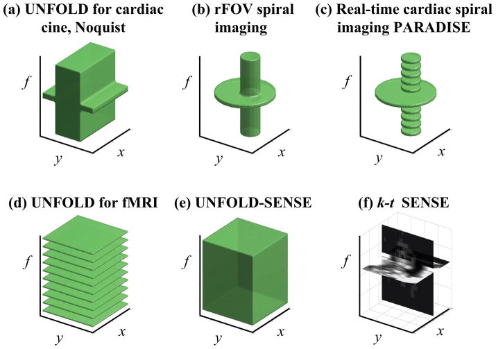
As depicted in Fig. 3, methods such as UNFOLD, UNFOLD-SENSE, PARADISE and several others involve regions of support in x-y-f space where non-aliased signal is expected and allowed. Spatial locations provided with a wide bandwidth along f can accommodate very dynamic temporal variations, while spatial locations provided with a narrow bandwidth can accommodate only static or nearly-static material. In a cardiac application for example, the heart would be located in the dynamic region for methods depicted in Fig. 3a–c. Periodic signals can be represented using only a subset of all frequencies (DC, the fundamental and all harmonics), and for this reason some applications like real-time cardiac imaging and fMRI where periodic signal variations are expected can be handled using discontinuous regions of support along the f axis (Fig. 3c–d). UNFOLD-SENSE makes very little assumptions, as it features regions of support that nearly cover the entire x-y-f volume and treat equivalently all x-y locations (Fig. 3e). Only the outer ~10% of the bandwidth along the f axis, near the Nyquist frequency, is not included into the UNFOLD-SENSE region of support.

Figure 3.

Prior knowledge about the imaged object can often be expressed in the form of a region of support in x-y-f space, where non-aliased signal is expected/allowed. A few examples are given here, for a few different dynamic imaging methods. A cube encompassing the whole FOV along x and y and bandwidth along f would represents full support, i.e., no assumption. The (x,y) locations provided with a wide bandwidth along f may contain very dynamic material, such as a beating heart, while locations provided with a narrow bandwidth can accommodate only nearly-static materials. A discontinuous support along f is appropriate in applications where the expected signal is periodic in time, giving rise to harmonics along f. When combined with parallel imaging, a nearly-full volume can be supported (about 90% of the f axis). In k-t SENSE, the prior knowledge can take instead the form of a low-resolution image.

Training data

k-t SENSE on the other hand uses a much richer set of prior knowledge, using actual image data rather than regions of support (Fig. 3f). This prior knowledge is cleverly used in the form of a regularization term, as part of the reconstruction equation (Eq. 12). In our results, the use of the M-based Tikhonov regularization at high acceleration settings proved much superior to ZTR. By using the M regularization matrix rather than ZTR in UNFOLD-SENSE and UNFOLD SPACE-RIP reconstructions as part of the O_l{} and O_r{} parallel imaging operators (Eq. 9), a (k-t SENSE)-(UNFOLD-SENSE) hybrid called hybrid-SENSE here was readily obtained.

6. Further information on the reconstruction algorithms used here

Scaling of the M regularization matrix

Because the calculation of the sensitivity S typically involves dividing the data from a given coil by data from all coils (15), the term S^HΨ⁻¹S in Eqs 11 and 12 is typically properly scaled, as any arbitrary scaling on the image magnitude would cancel out through the division. This is not the case however for the additive M⁻² regularization term, which can become larger or smaller and cause the system to become over- or under-regularized depending on arbitrary signal gains at the receive stage, or on whether a given FFT software applies scaling factors or not, for example. Under-regularized solutions are expected to be overly noisy, while over-regularized solutions are expected to introduce artifacts, making it important to strike the right balance. In analogy with ZTR, where a scalar may multiply an identity matrix with norm 1, we found it useful to divide the M matrix by its Froebinius norm, and multiply the result by a scalar that controls the amount of regularization performed. The regularization term thus becomes:

$${\lambda }^2{(\frac{\mathbf{M}}{{\left|\right|\mathbf{M}\left|\right|}_2})}^{-2}.$$ [13]

Retrospective cardiac cine reconstruction

The cardiac cine results presented here were reconstructed using retrospective gating, to properly capture the end-diastolic cardiac phases. Combining the temporal strategy in k-t SENSE and UNFOLD-SENSE with the temporal strategy in retrospective gating is not trivial, and an approach based on non-Cartesian sampling and the use of a conjugate gradient solver was presented in (18) for k-t SENSE. An alternative approach using various tricks to avoid the use of a solver (at least for the temporal direction) was presented in (19) for UNFOLD with parallel imaging, to reduce processing time by many-folds. Both approaches were implemented here for our (k-t SENSE)-(UNFOLD-SENSE) hybrid and very similar results were obtained from both.

Low spatial resolution data for sensitivity mapping and for M regularization

In the cardiac cine results presented here, a small central k-space region was used for sensitivity mapping and regularization purposes. While this central region could be fully sampled, we instead sub-sampled it by a factor of two in a way similar to ‘self, hybrid referencing with UNFOLD and GRAPPA’ (SHRUG) (4), for greater imaging speed. Because the sensitivity map of the imaged object is typically expected to be relatively static within a breath-hold experiment, the correlation between points near the very center of k-space is not expected to change in a dynamic way. A fully-populated region, only a few k-space lines wide, was obtained near k-space center through temporal filtering, and GRAPPA coefficients were calculated from this region as suggested in T-GRAPPA (20). GRAPPA was then used (21), with an acceleration factor of 2, to reconstruct the entire central region (typically about 10% of the k_y extent). This GRAPPA-reconstructed central region then allowed low-spatial resolution sensitivity maps as well as the regularization matrix M to be calculated. This self-calibration, self-referenced scheme is very reminiscent of the ‘GRAPPA-enhanced sensitivity maps for SENSE reconstructions’ (GEYSER) method presented in (22).

Materials and Methods

1. Phantom data

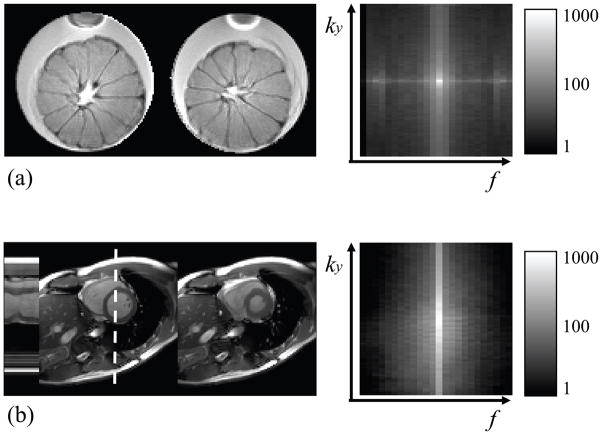
Phantom experiments were performed on a 3.0 T MR system equipped with manufacturer-supplied 8-channel head coil (GE Signa CVi, Milwaukee, WI) using a balanced steady state free precession (bSSFP) sequence, with TE = 2.4 ms, TR = 7 ms and FOV =12 cm. The receiver bandwidth was 125 kHz. The relatively long TR was a consequence of the relatively small object size and FOV. The phantom consisted of an orange immersed in a cylindrical water container, and the whole phantom was rotated to produce dynamic changes (see Fig. 4a). The phantom was imaged for several repetitions at each angular location, giving rise to a dataset featuring 24 frames of different rotations and 45 repetitions for each frame. Each one of the 45 equivalent datasets were undersampled and reconstructed independently. While data from only the first one were used to generate an MTF and to obtain the parameters for reconstruction, data from all 45 were used to measure a noise amplification ratio, as defined in Eq. 8. A second measure of the noise amplification ratio was also obtained through our Monte Carlo approach, using only the first dataset. The measure using all 45 acquired datasets was then compared to that from the Monte Carlo approach using only a single dataset, to validate the latter.

Figure 4.

(a) A phantom dataset with different rotations for different frames and (b) a cardiac cine dataset are displayed here. Temporal changes for the location indicated with a dotted line are plotted on the left, in (b). On the right, the datasets are represented in k_y-f space (root sum of mean square along k_x). As could be expected, much of the signal resides near the spatial and temporal DC region.

2. Fully-acquired in vivo data

Four fully sampled short-axis cardiac cine datasets were obtained, with informed consent and proper IRB approval, and were sub-sampled to simulate various acceleration factors (bSSFP sequence, product eight-channel cardiac array coil, flip angle = 45°, slice thichness = 7 mm, acquisition bandwidth = 125 kHz, TE/TR = 1.7/3.5 ms, 24 reconstructed phases). For faster processing, only the very dynamic region around the heart (e.g., see Fig. 4b) was used for MTF assessment purposes, as other regions featured mostly static signals and could not help the MTF evaluation beyond the immediate temporal DC region. The datasets with and without simulated perturbations (P_i,p in Eq. 5) were under-sampled according to both the UNFOLD-SENSE and k-t SENSE acceleration schemes, for various acceleration factors. A regulation factor λ of 3% was used (Eq. 13). Monte Carlo simulations using 45 iterations were performed to evaluate the noise amplification associated with each reconstruction. Although the different in vivo datasets were associated with significantly different anatomies and functions, the measured MTF, signal to noise ratio and noise enhancement were quite similar for all datasets and slices, suggesting our evaluation scheme does appear to be mostly object-independent, as expected and aimed for.

3. Accelerated in vivo data

Two subjects were imaged with an accelerated retrospective cardiac cine sequence, using the variable-density sampling strategy described in (4) (IRB-approved, short axis view, one subject at 3 T, flip angle = 45°, TR=4.0ms, TE=1.8ms, 7 mm thickness for 4 slices, matrix size = 192×160, and the other at 1.5 T, flip angle = 45°, TR = 3.5 ms, TE = 1.5 ms, 7 mm thickness for 6 slices, matrix size = 192×192. The images were acquired using the product 8-channel cardiac array coil equipped on each scanner. The skip factor for the outer k_y regions was either 4 (datasets at 1.5 T) or 8 (dataset at 3T), and only 2 near k-space center. The central region covered about 15% of the whole extent, enabling net acceleration factors of 3.5 and 6.3, respectively

Results

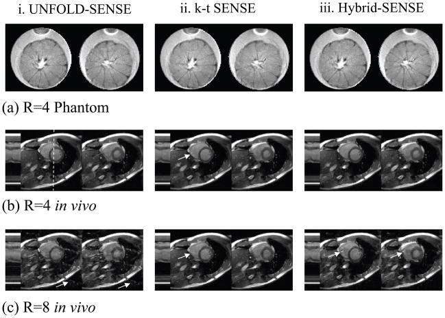
Figure 5 presents image results for two different acceleration settings (4-fold and 8-fold), three different reconstruction algorithms (UNFOLD-SENSE with ZTR, k-t SENSE and hybrid-SENSE), and two different datasets (phantom dataset and one of the downsampled in vivo datasets). In (b) and (c), the temporal changes for the line in the 2D spatial images that intersects the heart are also shown at the left.

Figure 5.

The reconstructed images for (a) the 4-fold undersampled phantom data, (b) the 4-fold and (c) 8-fold undersampled cardiac cine data are presented here. Arrows point to some of the main artifacts. In UNFOLD-schemes with ZTR, artifacts were found to be more static and related to the parallel imaging reconstruction near temporal DC. With k-t SENSE, artifacts were related to missing temporal frequencies.

1. 2D MTF results

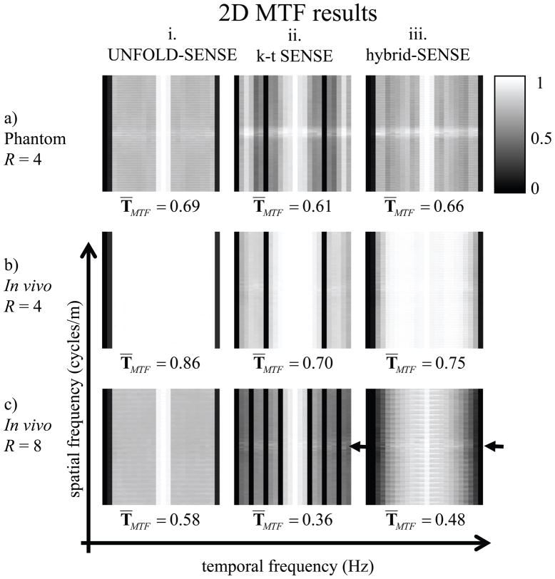
Figure 6 presents the 2D MTF results associated with the image reconstructions in Fig. 5. A perfect imaging method would be characterized by a uniform 2D MTF, equal to one at all spatial and temporal frequency locations. As could be expected, the MTF tends to be more degraded for a higher (8-fold) acceleration than for a lower (4-fold) one, for all methods. Looking either at Fig. 6 or the associated image results from Fig. 5, it can be seen that UNFOLD-SENSE with ZTR was most degraded evolving from good quality to artifact-plagued as the acceleration factor increases. The regularization scheme from k-t SENSE performed better than ZTR at higher acceleration. A main advantage of the k-t SENSE regularization scheme, used both in k-t SENSE and in hybrid-SENSE, can be seen in the form of a faint horizontal line near k_y=0 in Fig. 6c (see arrows), reflecting a better ability to capture low spatial frequencies.

Figure 6.

2D MTFs are presented for the three scenarios from Fig. 5: (a) phantom data at acceleration R=4, (b) in-vivo data at R=4 and (c) R=8. T̄_MTF was defined by the average of the overall T_MTF. Banding structure along the spatial frequency axis and sharp transitions along the temporal frequency axis can be observed in UNFOLD-SENSE with ZTR. The k-t SENSE results feature a greater ability at capturing the spatial low-frequency region (see brighter horizontal band, pointed to by a black arrow) and difficulty to capture some temporal frequencies (see black vertical bands). The hybrid method (Hybrid SENSE) appears to combine desirable features from both approaches, as it captures a continuous region along the temporal frequency axis and captures well the low-spatial frequency region (see black arrow).

A main advantage of the UNFOLD-SENSE acquisition scheme, used both in UNFOLD-SENSE with ZTR and in hybrid-SENSE, is the continuous coverage of the entire temporal frequencies axis except for a region around Nyquist. The k-t SENSE method, on the other hand, features R−1 blind frequency values for a sub-sampling factor of R, as can be understood from Fig. 2 and associated text. Because signals are not expected to be smooth along the temporal frequency axis, these missing locations may not be reliably recoverable through interpolation. With increased acceleration, the missing frequencies increase in number and get closer to the signal-rich f = 0 region, leading to a reduction in signal fidelity. Hybrid-SENSE combined desirable properties from both k-t SENSE and UNFOLD-SENSE, as can be seen from the higher-intensity horizontal lines near k_y = 0 and the continuous coverage along f in Fig. 6c.iii.

2. Artifact measurement results

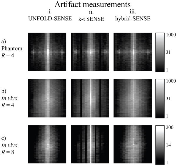
Figure 7 presents signal-to-artifact-ratio results calculated through Eq. 7 and associated with the image results and MTF results from Figs 5 and 6. A main strength of k-t SENSE can be seen from Figs 7b.ii and 7c.ii in the form of a bright line at f = 0. This feature can be understood from Fig. 2b and associated text, as nearly all aliased energy is displaced from the f = 0 location and the corresponding non-aliased signal can be recovered without any further processing. In contrast, UNFOLD-SENSE does not displace all overlapped signals away from DC (Fig. 2a), and still partly relies on parallel imaging to recover the f = 0 location.

Figure 7.

Maps of signal-to-artifact ratios are presented for the same scenarios as in Fig. 6. With a subsampling factor of 4, similar results were obtained for all tested methods. As acceleration increases, deviations between UNFOLD-SENSE with ZTR and k-t SENSE become clearer. See text for more details.

While aliased energy can be displaced along the temporal frequency axis, it must of course appear somewhere. Spreading aliasing components throughout the bandwidth causes some frequency locations to be missed (red bands in Fig. 2b and black bands in Fig. 6c.ii), but may allow a high signal-to-artifact ratio at the f = 0 location (Fig. 7c.ii). On the other hand, displacing half the components to Nyquist and keeping the others at DC allows a continuous bandwidth to be recovered (Fig. 2a and Fig. 6c.iii), but may lead to a lower signal-to-artifact ratio at the f = 0 location (Fig. 7c.iii). Accordingly, as acceleration is increased, k-t SENSE tends to gradually fail due to a loss in signal fidelity that comes from an increasing number of temporal frequency locations being missed, while UNFOLD-SENSE with ZTR and hybrid-SENSE tend to fail due to an increasingly large amount of DC artifacts obscuring the underlying anatomy.

Unlike MTFs, signal-to-artifact-ratio maps depend on the actual signal, which in turn depends on the object being imaged. Maps in Fig. 7a may appear different from those in Fig. 7b and 7c because the phantom used in Fig. 7a looks very different from the short axis cardiac images used in Figs 7b and 7c. While signal-to-artifact-ratio maps can be useful for comparing results from different methods or different reconstruction settings, they cannot reliably be used to compare results from different objects.

3. Noise measurement results

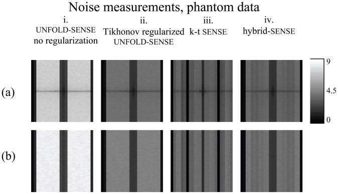
Figure 8 presents noise measurement results for the phantom experiment, calculated in two different ways: From the 45 repetitions (Eq. 13, Fig. 8a), and from our Monte Carlo approach using the information from the first repetition only (Fig. 8b). The purpose of Fig. 8 is to validate the Monte Carlo approach, so that noise measurements might then be presented for other datasets acquired without multiple repetitions.

Figure 8.

Noise amplification map, in k_y-f space, were measured on phantom data in two different ways: (a) Using 45 repetitive measurements, and (b) using a single repetition and a Monte Carlo approach. For all tested methods, (i) unregularized UNFOLD-SENSE, (ii) UNFOLD-SENSE with ZTR, (iii) k-t SENSE and (iv) hybrid-SENSE, both noise-amplification measurement methods gave essentially identical results, except for a central darker band in (a) associated with signal instability in repetitive measurements on our scanner. These results are interpreted here as a successful validation of the Monte Carlo approach.

Results from Fig. 8a and 8b are strikingly similar, except for a darker band near k_y = 0 in Fig. 8a. We have found these dark bands to be caused by instabilities in our scanner that induce signal, and not only noise, to vary from repetition to repetition. These field instabilities tended to affect the whole object globally and impacted mostly the k_y = 0 region in Fig. 8a. As they tended to increase both the numerator and denominator in Eq. 8 by a similar additive term, these instabilities made the ratio smaller and the corresponding entries darker in Fig. 8a. As the only substantial differences between Fig. 8a and Fig 8b were traced to hardware imperfections, we interpret the results in Fig. 8 as a successful validation of the Monte Carlo approach.

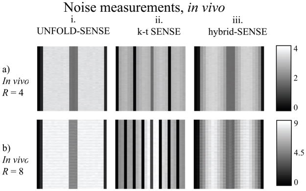
Figure 9 illustrates the noise amplification factor as measured through the Monte Carlo approach, from an in vivo dataset. The DC region where signals were reconstructed using a lower acceleration factor are associated with lower noise amplification, as could be expected. Such DC region is larger in UNFOLD-SENSE (about 10% of the bandwidth) and narrower with k-t SENSE (only the f = 0 location), it has a value of exactly the square root of the acceleration factor with k-t SENSE and can be higher in UNFOLD-SENSE. Variations along both spatial and temporal dimensions imply that the noise is neither spatially nor temporally homogeneous in the reconstructed images. The results in Fig. 9 are highly dependent on the amount of regularization used, i.e., the chosen value for λ (Eq. 13). Lower noise amplification can be readily obtained, at the price of extra blurring, by increasing λ. Compared to UNFOLD-SENSE and hybrid-SENSE, k-t SENSE had a tendency to have less noise amplification at f = 0, more noise amplification at locations near (but not equal to) f = 0, and less amplification at higher frequencies.

Figure 9.

Noise amplification maps, for the in-vivo data, were evaluated using the Monte Carlo approach. Lower acceleration settings at or near DC are associated with smaller noise amplification. The k-t SENSE regularization scheme allowed good noise suppression at high temporal frequencies (a.ii and b.ii), while UNFOLD-SENSE with ZTR performed well at low temporal frequencies (a.i and b.i). The performance of hybrid-SENSE (a.iii and b.iii), not surprisingly, is a compromise between the two other methods.

4. In vivo image results

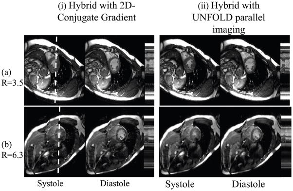
Data were acquired according to our proposed hybrid-SENSE scheme, with a sub-sampling factor of two near k-space center for sensitivity mapping and regularization purposes. The outer k-space regions were sub-sampled by a factor of either 4 or 8, for a net acceleration of 3.5 or 6.3, respectively. Results for two cardiac phases (mid-systole and mid-diastole) are presented in Fig. 10, for both datasets. The acquired data were reconstructed using two different algorithms that allow for retrospective cardiac gating, one originally proposed in conjunction with but not restricted to k-t SENSE (18) (left half of Fig. 10) using 2D conjugate gradients, and one originally proposed in conjunction with but not restricted to UNFOLD parallel imaging (19) (right half of Fig. 10). Especially in the presence of arrhythmia, elaborate non-linear schemes may be employed to map acquired time points onto a cardiac phase axis, and both approaches are equally capable of handling such schemes. Both approaches provided essentially equivalent results, although the one from (19) processed about 8 times faster. A combination of GRAPPA and SPACE RIP were used for reconstruction of the low and high temporal frequencies, respectively.(23) Artifacts, especially visible in the higher-acceleration case, were found to be nearly static, as expected and previously mentioned (Fig. 2a and Fig. 7c.iii).

Figure 10.

While other results in this work were obtained from subsampled versions of fully-sampled datasets, truly accelerated results are presented here. The results were reconstructed using our proposed hybrid approach, and could not be reconstructed with k-t SENSE as it requires a different subsampling scheme (see Fig. 2). Datasets were acquired for an acceleration factor of 3.5 (4-fold undersampling in outer k-space and 2-fold near center), and 6.3 (eight-fold in outer k-space and 2-fold near center). Two different retrospective-gating reconstruction strategies were implemented and provided equivalent results, although one processed about an order of magnitude faster. See text for more details.

Discussion

The present work was aimed at developing an object- and application-independent methodology to evaluate the performance of dynamic imaging methods. The output consists of easy-to-interpret 2D renderings that capture the frequency-dependent properties of given methods in terms of signal, artifacts and noise, as a function of spatial (k) and temporal (f) frequencies. Our analysis tools demonstrate the performance degradation that occurs in each reconstruction method with increasing acceleration (e.g., R = 8 in Fig. 6c compared to R = 4 in Fig. 6b). Performance of reconstruction algorithm also varied with the general setup, e.g., acceleration proved harder to achieve in the small-FOV phantom application than in the larger-FOV in vivo results (e.g., Fig. 6a compared to Fig. 6b). Variations were also found from method to method (e.g., Fig. 6c.i compared to Figs 6c.ii and 6c.iii). For the setup used here (i.e., given coil array and FOV) and a given dynamic imaging method, very little variations were found in results from different slices and volunteers, which is consistent of an object-independent evaluation. However, because these methods depend on the acquired data for self-calibration purposes and sometimes for regularization purposes as well, the evaluation of these methods could never be entirely object-independent.

Comparing results from different methods proved instructive in terms of visualizing and quantifying their main strengths and weaknesses. Methods based on the UNFOLD-SENSE sampling scheme were capable of capturing an uninterrupted temporal bandwidth (Fig 6a–c.i), but they can be vulnerable to static parallel-imaging artifacts (Fig 7a–c.i). On the other hand, with k-t SENSE, R-1 problematic locations were created along the temporal frequency axis where signal cannot be accurately recovered (Fig 6a–c.ii). While static parallel-imaging artifacts are mostly avoided by not performing any parallel imaging reconstruction on the DC component (Fig 7a–c.ii), the approach is vulnerable to overall losses in signal fidelity from these missing frequency locations. With respect to regularization schemes, the prior-knowledge based scheme from k-t SENSE proved useful at higher acceleration settings to maintain image quality, as compared to ZTR. This regularization scheme, from k-t SENSE, also proved entirely compatible with the sampling scheme from UNFOLD-SENSE, leading to the hybrid method proposed here. Our results suggest that the hybrid method advantageously combined desirable characteristics from both previous methods, as it captured continuous temporal frequency bandwidths while exploiting prior knowledge to maintain performance at higher acceleration settings.

Because the evaluation process requires the knowledge of a ‘truth’, and because different methods sub-sample k-space differently, the evaluation work had to be performed using datasets that were fully sampled and then sub-sampled at the reconstruction stage. Nevertheless, results were also presented that were actually acquired in an accelerated fashion (Fig. 10), and reconstructed using the proposed hybrid method. Reconstruction with k-t SENSE could not be performed on these datasets, as they were acquired using the UNFOLD-SENSE sampling scheme. Because these were cardiac cine datasets, two different retrospective-gating algorithms could be chosen for their reconstruction. One was proposed as part of k-t SENSE work but is not specific to k-t SENSE, and one was proposed as part of UNFOLD-SENSE work but is not specific to UNFOLD-SENSE. Both were found to provide similar results, although the one from (19) had a processing speed several-fold faster with a same conjugate gradient kernel. To enhance the performance of the proposed hybrid method, the parallel imaging part of the reconstruction algorithm was replaced by a combination of GRAPPA and SPACE RIP. GRAPPA was used to generate the sensitivity maps and the training data from the under-sampled central k-space region in a way similar to GEYSER (22), and to reconstruct signals in the region near temporal DC. SPACE RIP was used to reconstruct signal at higher temporal frequencies, as described in (23).

A notable limitation of the present evaluation method comes from the fact it is based on a linear problem (Eq. 3). Accordingly, the treatment of nonlinear algorithms such as compressed sensing appears to be beyond the scope of this work. The proposed methodology can handle reconstruction methods and regularization schemes that can be expressed in matrix form, but not the L₁-norm regularization scheme from compressed sensing. By assuming sparsity, signal perturbations may or may not be thoroughly ignored by the regularization scheme in Compressed Sensing, making the evaluation of a 2D MTF problematic. A more general evaluation strategy may be required to handle such non-linear algorithms. Computation effort represents another potential drawback. In the proposed approach, perturbations for the MTF calculations are introduced one at a time, leading to multiple reconstructions. But once an evaluation is complete, it should be relevant to any application of the method under test, as the evaluation tool extracts algorithm-dependent features and is mostly object-independent. As a further limitation, the present noise-estimation tool neglected noise correlation, which may be significant especially with arrays featuring large numbers of coil elements. The inclusion of measured pre-scan noise data, as done in (16), could in principle improve our noise estimates in terms of accuracy. Finally, while k-f representations were found most informative for the methods tested here, it should be noted that alternative representations, e.g., in the x-f space, would be readily obtainable through minor modifications to the proposed algorithms and could prove helpful in given situations.

Conclusions

An approach to evaluate in a visually intuitive way the performance of dynamic imaging methods in terms of 2D MTF, signal to noise ratio and noise amplification was presented. A hybrid method that combines the main desirable characteristics observed from k-t SENSE and UNFOLD-SENSE was introduced.

References

- 1.Madore B, Glover GH, Pelc NJ. Unaliasing by fourier-encoding the overlaps using the temporal dimension (UNFOLD), applied to cardiac imaging and fMRI. Magn Reson Med. 1999;42:813–828. doi: 10.1002/(sici)1522-2594(199911)42:5<813::aid-mrm1>3.0.co;2-s. [DOI] [PubMed] [Google Scholar]
- 2.Tsao J, Boesiger P, Pruessmann KP. k-t BLAST and k-t SENSE: dynamic MRI with high frame rate exploiting spatiotemporal correlations. Magn Reson Med. 2003;50:1031–1042. doi: 10.1002/mrm.10611. [DOI] [PubMed] [Google Scholar]
- 3.Kellman P, Epstein FH, McVeigh ER. Adaptive sensitivity encoding incorporating temporal filtering (TSENSE) Magn Reson Med. 2001;45:846–852. doi: 10.1002/mrm.1113. [DOI] [PubMed] [Google Scholar]
- 4.Madore B. UNFOLD-SENSE: a parallel MRI method with self-calibration and artifact suppression. Magn Reson Med. 2004;52:310–320. doi: 10.1002/mrm.20133. [DOI] [PubMed] [Google Scholar]
- 5.Sharif B, Aggarwal N, Bresler Y. PARADISE: Patient-adaptive reconstruction and acquisition in dynamic imaging with sensitivity encoding. Proceedings of Joint Annual Meeting ISMRM-ESMRMB; Berlin, Germany. 2007. p. 151. [Google Scholar]
- 6.Prieto C, Batchelor PG, Hill DL, Hajnal JV, Guarini M, Irarrazaval P. Reconstruction of undersampled dynamic images by modeling the motion of object elements. Magn Reson Med. 2007;57:939–949. doi: 10.1002/mrm.21222. [DOI] [PubMed] [Google Scholar]
- 7.van Vaals JJ, Brummer ME, Dixon WT, Tuithof HH, Engels H, Nelson RC, Gerety BM, Chezmar JL, den Boer JA. “Keyhole” method for accelerating imaging of contrast agent uptake. J Magn Reson Imaging. 1993;3:671–675. doi: 10.1002/jmri.1880030419. [DOI] [PubMed] [Google Scholar]
- 8.Malik SJ, Schmitz S, O’Regan D, Larkman DJ, Hajnal JV. x-f Choice: reconstruction of undersampled dynamic MRI by data-driven alias rejection applied to contrast-enhanced angiography. Magn Reson Med. 2006;56:811–823. doi: 10.1002/mrm.21008. [DOI] [PubMed] [Google Scholar]
- 9.Brummer ME, Moratal-Perez D, Hong CY, Pettigrew RI, Millet-Roig J, Dixon WT. Noquist: reduced field-of-view imaging by direct Fourier inversion. Magn Reson Med. 2004;51:331–342. doi: 10.1002/mrm.10694. [DOI] [PubMed] [Google Scholar]
- 10.Korosec FR, Frayne R, Grist TM, Mistretta CA. Time-resolved contrast-enhanced 3D MR angiography. Magn Reson Med. 1996;36:345–351. doi: 10.1002/mrm.1910360304. [DOI] [PubMed] [Google Scholar]
- 11.Wu Y, Jeong EK, Parker DL, Alexander AL. UNFOLD using a temporal subtraction and spectral energy comparison technique. Magn Reson Med. 2002;48:559–564. doi: 10.1002/mrm.10247. [DOI] [PubMed] [Google Scholar]
- 12.Thunberg P, Zetterberg P. Noise distribution in SENSE- and GRAPPA-reconstructed images: a computer simulation study. Magn Reson Imaging. 2007;25:1089–1094. doi: 10.1016/j.mri.2006.11.003. [DOI] [PubMed] [Google Scholar]
- 13.Madore B. Dynamic Imaging Methods Assessed with A 2D MTF Approach. Proceedings of the 16th Annual Meeting of ISMRM; Toronto, Canada. 2008. p. 1496. [Google Scholar]
- 14.Madore B. Using UNFOLD to remove artifacts in parallel imaging and in partial-Fourier imaging. Magn Reson Med. 2002;48:493–501. doi: 10.1002/mrm.10229. [DOI] [PubMed] [Google Scholar]
- 15.Pruessmann KP, Weiger M, Scheidegger MB, Boesiger P. SENSE: sensitivity encoding for fast MRI. Magn Reson Med. 1999;42:952–962. [PubMed] [Google Scholar]
- 16.Kellman P, McVeigh ER. Image reconstruction in SNR units: a general method for SNR measurement. Magn Reson Med. 2005;54:1439–1447. doi: 10.1002/mrm.20713. [DOI] [PMC free article] [PubMed] [Google Scholar]
- 17.King KF, Angelos A. SENSE image quality improvment using matrix regularization. Proceedings of the 9th Annual Meeting of ISMRM; Glasgo, Scotland. 2001. p. 1771. [Google Scholar]
- 18.Hansen MS, Baltes C, Tsao J, Kozerke S, Pruessmann KP, Eggers H. k-t BLAST reconstruction from non-Cartesian k-t space sampling. Magn Reson Med. 2006;55:85–91. doi: 10.1002/mrm.20734. [DOI] [PubMed] [Google Scholar]
- 19.Madore B, Chu R, Zientara GP. Accelerated cardiac cine imaging, with retrospective gating. ISMRM 14th Scientific Meeting & Exhibition; Seattle, Washington, USA. 2006. p. 763. [Google Scholar]
- 20.Breuer FA, Kellman P, Griswold MA, Jakob PM. Dynamic autocalibrated parallel imaging using temporal GRAPPA (TGRAPPA) Magn Reson Med. 2005;53:981–985. doi: 10.1002/mrm.20430. [DOI] [PubMed] [Google Scholar]
- 21.Griswold MA, Jakob PM, Heidemann RM, Nittka M, Jellus V, Wang J, Kiefer B, Haase A. Generalized autocalibrating partially parallel acquisitions (GRAPPA) Magn Reson Med. 2002;47:1202–1210. doi: 10.1002/mrm.10171. [DOI] [PubMed] [Google Scholar]
- 22.Hoge WS, Brooks DH. Using GRAPPA to improve autocalibrated coil sensitivity estimation for the SENSE family of parallel imaging reconstruction algorithms. Magn Reson Med. 2008;60:462–467. doi: 10.1002/mrm.21634. [DOI] [PMC free article] [PubMed] [Google Scholar]
- 23.Chao TC, Hoge WS, Madore B, Yuan J, Chung HW. Reconstruction of retrospectively-gated cardiac data using a combination of GRAPPA, SPACE-RIP, UNFOLD and an adaptive regularization scheme. Proceedings of the 17th Annual Meeting of ISMRM; Honolulu, Hawaii, USA. 2009. p. 4566. [Google Scholar]