Unifying Vertical and Nonvertical Evolution: A Stochastic ARG-based Framework

Abstract

Evolutionary biologists have introduced numerous statistical approaches to explore nonvertical evolution, such as horizontal gene transfer, recombination, and genomic reassortment, through collections of Markov-dependent gene trees. These tree collections allow for inference of nonvertical evolution, but only indirectly, making findings difficult to interpret and models difficult to generalize. An alternative approach to explore nonvertical evolution relies on phylogenetic networks. These networks provide a framework to model nonvertical evolution but leave unanswered questions such as the statistical significance of specific nonvertical events. In this paper, we begin to correct the shortcomings of both approaches by introducing the “stochastic model for reassortment and transfer events” (SMARTIE) drawing upon ancestral recombination graphs (ARGs). ARGs are directed graphs that allow for formal probabilistic inference on vertical speciation events and nonvertical evolutionary events. We apply SMARTIE to phylogenetic data. Because of this, we can typically infer a single most probable ARG, avoiding coarse population dynamic summary statistics. In addition, a focus on phylogenetic data suggests novel probability distributions on ARGs. To make inference with our model, we develop a reversible jump Markov chain Monte Carlo sampler to approximate the posterior distribution of SMARTIE. Using the BEAST phylogenetic software as a foundation, the sampler employs a parallel computing approach that allows for inference on large-scale data sets. To demonstrate SMARTIE, we explore 2 separate phylogenetic applications, one involving pathogenic Leptospirochete and the other Saccharomyces.

The transfer of genetic material through nonvertical phenomena plays a significant role in evolution and evolutionary theory. Examples include horizontal gene transfer (HGT) in bacteria, archeabacteria, unicellular eukaryotic organisms, plants, and metazoans (Lawrence and Ochman 1998; Nelson et al. 1999; Andersson et al. 2003; Richardson and Palmer 2007; Gladyshev et al. 2008); recombination and reassortment in viruses (Temin 1991; Nelson and Holmes 2007; Wilson et al. 2009); hybridization and introgression in both plants and animals (Buckley et al. 2006; Mallet 2007); and meiotic recombination in eukaryotes (McVean et al. 2004).

As little as 30 years ago, biologists generally lent little credit to nonvertical events in shaping evolution, believing these to be extremely rare (Doolittle 1999). But with the move into the genomic era in biology, biologists have discovered widespread instances of nonvertical evolution, causing them to rethink several fundamental biological theories, including a universal tree of life (Wolf et al. 2002; Doolittle and Bapteste 2007) and neo-Darwinian evolution (Koonin 2009). In addition to a central role in evolutionary theory, nonvertical evolution also has numerous public health implications (Brown 2003). For example, in the past century genomic reassortment has been directly associated with major influenza A pandemics in 1957 and 1968 (Lindstrom et al. 2004). More recently, genomic reassortment has rendered the drug amantadine ineffective against circulating influenza A virus (Bright et al. 2006; Simonsen et al. 2007), causing researchers to question the effectiveness of the drug oseltamivir in the event of a major influenza H5N1 avian influenza epidemic (Simonsen et al. 2007; Enserink 2009). In addition to reassortment, homologous recombination plays a significant role in the emergence of drug-resistant HIV virions (Rambaut et al. 2004; Nora et al. 2007), and in microbes, HGT has been the dominant force in the emergence of the multidrug-resistant bacteria Enterobacteriaceae (Leverstein-van Hall et al. 2002).

With such pressing public health concerns and with such a central role in biology, it becomes worrisome that methods to infer and examine nonvertical transmission events remain limited (Philippe et al. 2005). Methodological progress on these problems is being made in population genetic, phylogenetic, and computational biology contexts, but no unified model exists to conduct formal statistical inference on both vertical and nonvertical evolution (Edwards et al. 2007; Woolley et al. 2008).

One popular approach to examine nonvertical evolution relies on gene-tree incongruence (Posada et al. 2002). This approach attempts to find discordance between phylogenetic trees inferred from different genes or loci because discordance is one possible signal of nonvertical evolution (Grassly and Holmes 1997). In terms of formal models for this approach, Ané et al. (2007) introduce a statistical methodology to estimate concordance factors between trees (Baum 2007) using importance sampling. In a recent work, Åkerborg et al. (2009) adopt a species-tree framework for gene-tree reconciliation. Minin et al. (2005), Suchard et al. (2005), and Bloomquist et al. (2009) adopt a Markov chain Monte Carlo (MCMC) approach to make inference through a Bayesian multiple change-point model that simultaneously models gene-tree variability and spatial evolutionary changes across genomic regions. Husmeier and McGuire (2003) exploit a similar approach using hidden Markov models.

These formal phylogenetic statistical models provide information on gene-tree incongruence but at a potentially high scientific cost. For example, gene-tree incongruence does not provide information on the dates of nonvertical events. Most troublesome about these methods is that rather than modeling nonvertical events in a single unified structure, these methods look at collections of, at most, Markov-dependent, bifurcating trees, where this dependence lies almost exclusively on the topological shape. These tree collections provide some information on nonvertical events, but only indirectly, making findings difficult to interpret and generalize. Moreover, reliance on tree collections oftentimes leads to ad hoc or heuristic modeling frameworks that do not lend themselves to further generalizations (Ané et al. 2007; Bloomquist et al. 2009). In addition to these modeling considerations, weak dependence assumptions in these methodologies forsake a hierarchical framework, diminishing statistical power to detect significant differences (Suchard, Kitchen, et al. 2003).

An alternative approach, relatively unexplored in the phylogenetics literature, but highly popular in population genetics, entertains ancestral recombination graphs (ARGs). First proposed by Hudson (1983), an ARG 𝒢 is a directed graph that simultaneously describes both vertical and nonvertical evolutionary events. Because of this, an ARG addresses the issues plaguing the gene-tree incongruence framework. Within the past decade, population genetics has enjoyed an explosion of research about ARG inference and the associated coalescent with recombination (CWR) of Hudson (1983). One major area has been the estimation of population size N_e and recombination rate ρ using the CWR and likelihood-based inference. Theoretically sound and more powerful than previous attempts (Wall 2000), likelihood-based inference on the CWR requires extremely difficult calculations. To derive the likelihood of genetic data Y given population size N_e and recombination rate ρ, p(Y|N_e,ρ), researchers use basic probability to average over all possible ARGs. More succinctly, researchers first propose a likelihood computed assuming an infinite-sites model, p(Y|𝒢), and then using the CWR, p(𝒢|N_e,ρ), researchers take advantage of

(1)

to find the marginal likelihood (Felsenstein et al. 1999). Regardless of the statistical framework used to make inference on this distribution, calculation of this quantity requires a summation over the astronomically large space of ARGs. It simply cannot be done directly using modern computing technology. To remedy this difficulty, researchers have proposed numerous alternative inference procedures (Stumpf and McVean 2003). Building from the earlier works of Griffiths and Marjoram (1996) and Stephens and Donnelly (2000), Fearnhead and Donnelly (2001) present a vastly improved importance sampler (Felsenstein et al. 1999) to make inference on N_e and ρ. More recently, Griffiths et al. (2008) improve upon Fearnhead and Donnelly (2001) using the diffusion approximation techniques of De Iorio and Griffiths (2004). Kuhner et al. (2000) and Nielsen (2000) embrace MCMC so as to focus attention on ARGs with significant contribution to p(Y|N_e,ρ). Also using MCMC, Wang and Rannala (2008) present a computationally efficient methodology to infer the distribution ρ along the genome, with implications for hot-spot mapping. Using a similar limiting strategy but in a deterministic framework, Lyngsø et al. (2008) limit the summation by enumerating ancestral configurations. A final approach circumvents these calculations altogether by approximating the likelihood using a product of approximate conditionals (Li and Stephens 2003; McVean and Cardin 2005). Hudson (2001) and Fearnhead and Donelly (2002) present alternative composite likelihood approximations.

The adoption of ARGs in population genetics has resulted in numerous scientific advances (McVean et al. 2004; Myers et al. 2005; Winckler et al. 2005). Little work in population genetics, however, focuses on the ARG as the primary parameter of interest. This occurs for multiple reasons. First, ARGs remain in their infancy and much research remains to be done. Second, population genetics deals with the contributions of mutation, natural selection, genetic drift, and population structure on genetic variation, relegating the ARG to secondary importance (Wakeley 2005). Finally, population genetics usually concentrates on data with relatively low divergence levels, making the recovery of the true ARG nearly impossible (Kuhner et al. 2000). Instead most work in population genetics treats the ARG as a nuisance parameter and attempts to integrate it out of the model completely.

In addition to the 2 communities mentioned above, the phylogenetic network community also deals extensively with nonvertical evolution. Recognizing that ARGs are graph-theoretic objects distinct from the coalescent framework, this computational biology community has abstracted the definition of an ARG into a phylogenetic network. Using definitions suggested by Huson and Bryant (2006), ARGs simply represent a special type of “explicit” or “reticulate” network. Other network types include “median networks” and “consensus networks” that fall under the category of “splits networks”. Over the past 10 years, the phylogenetic network community has grown quite fast and numerous applied and theoretical advances have been made (Baroni et al. 2004; Gusfield et al. 2004; Song and Hein 2005; Huson and Bryant 2006; Bordewich and Semple 2007; Wu et al. 2008). Much work remains to be completed, but the field shows much promise (Woolley et al. 2008).

Bearing closest relation to our work, the phylogenetic network community has taken 2 complimentary approaches to infer nonvertical evolution using explicit networks. The first adopts a parsimony approach and attempts to find the minimum number of nonvertical events that explain a particular evolutionary history (Hudson and Kaplan 1985; Hein 1993; Wang et al. 2001; Gusfield et al. 2004; Song and Hein 2005; Jin et al. 2007). The second approach adopts a statistical framework punctuated by a formal stochastic model. Early work by Strimmer et al. (2001) adopts a Bayesian framework for inference and later work by Jin et al. (2006) provides a method to find the maximum likelihood network. In another recent work, Didelot and Falush (2007) provide a joint model for vertical evolution and recombination but avoids modeling the origin of the nonvertically transferred genetic information. All 3 methods provide a framework to jointly model vertical and nonvertical evolution but leave unanswered questions such as the statistical significance of specific nonvertical events.

In our current work, we blend and unify ideas from much of the above into the “stochastic model for reassortment and transfer events” (SMARTIE). In particular, we start with the Bayesian approach of Strimmer et al. (2001), mix in the hierarchical modeling approach of Suchard, Weiss, et al. (2003), and finally adopt a similar MCMC approach to Wang and Rannala (2008) to make inference. Novel to SMARTIE is an explicit Bayesian prior for inference on the number of nonvertical nodes, avoiding the use of the CWR commonly used in population genetics (Didelot and Falush 2007; Wang and Rannala 2008). Because of this, we provide a formal way to test and infer nonvertical evolution. For inference on our model, we implement an MCMC sampler in the BEAST phylogenetic software package of Drummond and Rambaut (2007) that uses the reversible jump methodology of Green (1995) to move within ARG space. In addition, we adopt a parallel processing component to compute the likelihood, increasing efficiency on large genomic data sets. To demonstrate our model, we analyze 2 empirical examples. The first examines a Leptospira interrogans data set in order to gain more information on the evolutionary history (Stevenson et al. 2007), and the second explores a Saccharomyces data set taken from Rokas et al. (2003). We conclude with a discussion of SMARTIE and its place in current molecular evolutionary research.

MODEL

Our data consist of M molecular sequence alignments, Y₁,…,Y_M, that we group into the multilocus vector Y = (Y₁,…,Y_M). Each alignment Y_m, for m = 1,…,M, contains sequence information on the same N taxa and has length S_m. We let Y_ms = (Y_ms1,Y_ms2,…,Y_msN)^′ denote homologous character columns of Y_m = (Y_m1,…,Y_ms,…,Y_mSm) and use s = 1,…,S_m to index columns (sites). Every element Y_msn for n = 1,…,N identifies a sequence character or standard ambiguity code, which allows for missing sequences for some taxa in the multilocus data set. Each alignment Y_m typically corresponds to a distinct biologically meaningful genomic unit—for example, a gene, a paralog, or an exon—suggested by Y and the research hypothesis.

Likelihood

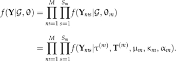
We take a statistical phylogenetic approach and assume each column Y_ms to be independent and identically distributed by the column sampling density f(Y_ms|ϑ) given unknown model parameters ϑ. In the classic phylogenetic setting, ϑ contains a bifurcating tree topology τ, a vector of branch length parameters T, and the parameters connecting the sequence characters to a stochastic substitution process, that is, a continuous-time Markov chain (CTMC). In the case of SMARTIE, however, we replace τ with an ARG 𝒢. An ARG is a directed graph that begins with a bifurcating root node at time t₀ > 0 and ends with N external tip nodes sampled at time 0. Between the first bifurcating root node at t₀ and our sampling time 0, 𝒢 contains R ≥ 0 nonvertical nodes representing nonvertical events and N + R − 2 bifurcation nodes representing vertical events. Nonvertical nodes receive complimentary genomic material from their 2 parental nodes, whereas bifurcation nodes pass their complete genomic material onto both of their children. Figure 1 displays an example of an ARG with N = 9 taxa and 1 nonvertical node (R = 1).

FIGURE 1.

Nonvertical evolution confirmation and event dating. The figure shows most probable ARG that represents the evolutionary history of 9 members of the lenfamily in Leptospira interrogans. For each of the taxa, the first letter represents the gene, for example, CNrepresents the lenCgene and DNrepresents the lenDgene. The second letter in each taxa describes whether the taxa represents the C-terminal or the N-terminal of the particular gene, for example, CNderives from the N-terminal of the lenCgene. The lenAgene only has an N-terminal. We abbreviate the L. interroganslineages as Hardjo (har), Grippotyphosa (gri), Canicola (can), Bratislava (bra), Pomona (pom), Copenhageni (cop), and Lai (lai). The white circles on the ARG represent bifurcation nodes, and the black circles represent nonvertical nodes. The dashed lines represent edges involved in a nonvertical event; the remaining solid lines represent edges not involved in a nonvertical event. The figure displays 95% credible intervals for the height of each node in parentheses in expected number of substitutions. We display confidence intervals for the heights of nodes (1,2,3) near the root of the ARG. SMARTIE provides a 90% posterior probability for this history. If we had used alternative gene-tree incongruence procedures, significance statements like this would not be possible.

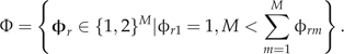
To develop the necessary notation, we define an “ordered” ARG 𝒢, or just an ARG, as the tuple (𝒱,ℰ,T,φ), where (𝒱,ℰ) are the node (vertex) and edge sets of a directed graph, T is a vector of node times, and φ is a nonvertical labeling parameter. The set 𝒱 contains 2N + 2R − 1 nodes. The vector T induces an ordering on 𝒱, with the root node corresponding to v₀. For each bifurcation node v_b ∈ 𝒱, ℰ contains the edges (v_b,v_c1(b)) and (v_b,v_c2(b)) with c₁(b) and c₂(b) identifying as the children of v_b. Similarly, ℰ contains the edges (v_p1(r),v_r) and (v_p2(r),v_r) for each nonvertical node v_r ∈ 𝒱, where p₁(r) and p₂(r) identify the parents of v_r. To incorporate multilocus data, we provide each node v_r ∈ 𝒱 with a partitioning parameter φ_r = (φ_r1,…,φ_rM) ∈ Φ ⊂ {1,2}^M that describes the inheritance of the 2M parental regions at v_r. A value of 1 for φ_rm says that partition m segregates with the first parent p₁(r) of v_r, whereas a value of 2 signifies the second parent p₂(r). ARGs can handle numerous instances of nonvertical evolution, so Φ can have multiple parameterizations depending upon the data at hand; we return to this point in the Prior Distribution section. We set the vector φ equal to (φ₁,…,φ_R). Our ARG definition generalizes the definition provided by Griffiths and Marjoram (1996). In their definition, they specify Φ according to a recombination partition structure; we discuss this facet more in the Prior Distribution section. Our definition of an ARG also falls under the category of an explicit network (Huson and Bryant 2006).

A multipartite ARG 𝒢 naturally induces a marginal bifurcating tree τ^(m) on every partition m. Griffiths and Marjoram (1996) provide an excellent description and introduction to this induction. Each marginal tree τ^(m) contains N − 1 bifurcation nodes, with consistent bifurcation times across the data partitions, and the associated vector of node times T^(m) subsets T, that is, T^(m) ⊂ T. Due to the structure of 𝒢, T^(m) does not automatically contain t₀. The vector τ equals the collection of marginal trees (τ⁽¹⁾,…,τ^(m)).

Using the induced marginal trees τ and branch lengths in T, we can directly compute the data likelihood using the peeling algorithm of Felsenstein (1981). To complete this computation, we specify a sequence character substitution process acting within each partition; specifically, we utilize CTMCs with instantaneous rate matrices Q_m. In general, the nature and type of data in each partition Y_m, be it nucleotide, amino acid, or codon, posit a parameterization for Q_m. Furthermore, due to alternative data types or other evolutionary phenomenon, each data partition Y_m may suggest its own unique parameterization for Q_m. In this paper, our data examples concentrate exclusively on nucleotide data, so we adopt the parameterization of Hasegawa et al. (1985) on every Q_m with discrete Γ-approximated rate variation (Yang 1994). We specify κ_m as the transition–transversion ratio, π_m = {π_Am,π_Gm,π_Cm,π_Tm} as the stationary distribution, and α_m as the rate variation parameter. We fix π_m equal to the estimated empirical frequencies _m of each alignment because π_m ≈ _m under most data situations (Li et al. 2000). We normalize Q_m so that rate scalar μ_m measures the expected number of substitutions per unit length on T^(m). We let θ_m = (μ_m,κ_m,α_m) and combine (κ₁,…,κ_m) into κ, (α₁,…,α_m) into α, (μ₁,…,μ_m) into μ, with θ = (θ₁,…,θ_m). Using this notation, the complete data likelihood can be written out as

(2)

We want to emphasize that every induced gene tree has its own clock rate, which allows for different branch lengths among the induced trees. To give an example of this, assume that we have N = 3 taxa (A,B,C) and M = 4 loci with relative clock rates μ = (0.8,0.9,1.1,1.2). Taxa B is a hybrid between taxa A and C with lineages at Loci 1 and 2 descending from A and Loci 3 and 4 descending from B. The induced trees for Locus 1 and Locus 2, τ⁽¹⁾ and τ⁽²⁾, are both ((A:1,B:1):1,C:2), and the induced trees for Loci 3 and 4, τ⁽³⁾ and τ⁽⁴⁾, are both (A:2,(B:1,C:1):1) in relative time units. We multiply these times by the locus-specific entries in μ. Thus, the rate tree for Locus 1 in expected number of substitutions per site equals ((A:0.8,B:0.8):0.8,C:1.6), the rate tree for Locus 2 equals ((A:0.9,B:0.9):0.9,C:1.8), the rate tree for Locus 3 equals (A:2.2,(B:1.1,C:1.1):1.1), and the rate tree for Locus 4 equals (A:2.4,(B:1.2,C:1.2):1.2).

In some sense, we can think about the relationship between 𝒢 and τ hierarchically. In particular, the ARG 𝒢 pools topological and branch length information from the M trees in τ. We note that this pooling does enforce a strict-like clock on each τ, and this may not be appropriate for all data sets (Strimmer et al. 2001). We discuss a possible extension to this idea in Discussion.

Prior Distribution

To complete model specification, we assume independent priors on θ and 𝒢. We follow phylogenetic hierarchical (Suchard, Kitchen, et al. 2003) practice and model each θ_m as

(3)

with ν = (ν_μ, ν_κ, ν_α) and Σ = diag(σ_μ²,σ_κ²,σ_α²). When M < 4, little information exists in the data about the variability across the partitions, so we fix ν and Σ; when M ≥ 4, we assume that ν and Σ are random and place the noninformative priors of Minin et al. (2005) over them. In either case, we fix ν_μ = 0 to ensure identifiability between μ and T in the posterior.

We now move to specifying a prior over the ARG 𝒢, beginning with the partitioning parameter Φ. SMARTIE provides a general framework for nonvertical inference through Φ. In particular, SMARTIE allows us to tailor Φ according to the application at hand. Three of the most popular parameterizations include reassortment, recombination, and single-gene conversion. A reassortment parameterization assumes that the partitions are unordered and independent. As such, reassortment allows the nonvertical node v_r corresponding to φ_r to freely select each parental partition without regard to the neighboring partitions. A recombination parameterization, however, requires that at a specific point, the partitions physically located to the left segregate from one parent and the partitions to the right segregate from the other. Lastly, a single-gene conversion parameterization allows for only a single locus to be transferred. More formally, under reassortment, we define the space of possible partitioning parameters as

(4)

The restriction φ_r1 = 1 preserves identifiability because the labelings of the first and second parent are arbitrary and the second restriction mandates that at least one partition comes from each parent, a reassortment event actually occurs. For the recombination parameterization, we define

(5)

Finally, for the single-gene conversion parameterization, we define

(6)

With a parameterization for Φ, we continue our prior specification by considering several densities over φ. The first is uniform over all possible partitions

(7)

and is appropriate when have no prior information on gene flow or nonvertical events. Unfortunately, when we parameterize Φ as a reassortment space, |Φ|^R grows exponentially in M, making inference incredibly difficult. One approach to counter this growth proposes that the number W_r of genes transferred in a single event should be small (Beiko and Ragan 2008). To reflect this prior belief, we consider

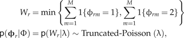(8)

where λ is the expected number of transferred genes. The number of transferred genes W_r must always be greater than 0 and less than , so we truncate the Poisson distribution accordingly. In extremely data-rich situations, more biologically intriguing hyperpriors on φ may be appropriate; we explore these possibilities in Discussion.

With a prior specification on φ, we move to the graph components of 𝒢. Currently, the CWR prior stands as the most popular prior choice. The CWR robustly encompasses a wide variety of evolutionary models in population genetics, including the Wright–Fisher (Fisher 1930; Wright 1931) and Moran models (Moran 1958). Consequentially, population geneticists almost exclusively rely on the CWR. This marriage between an ARG and the CWR, however, comes with a high cost because coalescent assumptions and approximations often fail (Donnelly and Tavaré 1995; Eldon and Wakeley 2006; Fu 2006). Springing from this observation, we introduce a relatively noninformative prior over 𝒢 for use in SMARTIE. This approach builds upon common Bayesian inference procedures in phylogenetics that assume a uniform distribution over tree topologies and exponential distribution over branch lengths. In particular, the prior breaks 𝒢 down into R, T, and (𝒱, ℰ) and then uses basic probability to write

(9)

The first portion of equation (9) assumes R ∼ Poisson(η),

(10)

where η represents our prior belief in the number of nonvertical transmission events. If we have little or no prior information, we typically set η = ln(2) so that before looking at the data, there is a 50-50 chance of at least one nonvertical event occurring. Given this prior for R, the second portion of equation (9) assumes that t₀ follows a noninformative Gamma(γ,δ) distribution and T − {t₀} has the same distribution as a collection of K − 1 ordered statistics from K − 1 independent Uniform(0, t₀) random variables,

(11)

The last portion of equation (9) assumes a uniform distribution over the topological relationships of the vertices,

(12)

where Ω_R,N is the total number of ordered ARGs 𝒢 that have N external tips and R nonvertical events. In Appendix 1, we describe a method to calculate this quantity.

Inference

Regardless of prior choice, we let Ψ be the vector of all hyperparameters and Θ = (𝒢,θ,Ψ) be the vector of all modeling parameters. Under a Bayesian framework, inference on Θ relies on the full posterior distribution p(Θ|Y) ∝ f(Y|θ,𝒢) × p(Θ). Simple to write down, this distribution remains intractable due to a large integration step when computing the proportionality constant. To handle this, we implement an MCMC sampler to draw random samples from the posterior distribution p(Θ|Y) (Liu 2001). We implement this sampler in the BEAST phylogenetic software package of Drummond and Rambaut (2007). The sampler exploits a variety of transition kernels to generate the Markov-dependent samples. For continuous parameters in Θ, the sampler uses standard adaptive transition kernels provided by BEAST. To move within the space of 𝒢, however, we develop 3 novel transition kernels. For fixed R, we consider a random walk kernel that moves within 𝒢 in a manner similar to the narrow exchange and subtree transfer operators of standard Bayesian phylogenetics (Lakner et al. 2008). To explore the variable dimensional space of 𝒢, the sampler employs a reversible jump kernel (Green 1995) to add and remove nonvertical events. The third kernel uses a random walk mechanism to explore φ. These kernels, plus those already in BEAST, guarantee that SMARTIE's MCMC chain satisfies irreducibility and reversibility. Further details of these transition kernels find themselves in Appendix 2.

When generating random samples from the posterior distribution, the sampler spends a majority of its time recomputing the data likelihood f(Y|𝒢,θ) given new positions in ARG space, even when using the peeling algorithm of Felsenstein (1981). To overcome this, applied investigators undertaking large phylogenetic analysis often resort to limiting the taxa size N or the sequence length S. A third option is parallel computing. In the past decade, several groups have developed algorithms and software interfaces for parallel phylogenetic reconstruction techniques. These include DRPml (Keane et al. 2005), pIQPNNI (Minh et al. 2005), RAxML-III (Stamatakis et al. 2005), fastDNAml (Stewart et al. 2001), ASA (Zhou and Jermiin 2004), GRAPPA (Moret et al. 2002), MrBayes (Altekar et al. 2004), PBPI (Feng et al. 2003), TREE-PUZZLE (Schmidt et al. 2002), and BEAGLE (Suchard and Rambaut 2009). These parallel methods provide dramatic runtime improvements for phylogenetic reconstruction, making large analyses computationally possible (Stamatakis et al. 2004; Feng et al. 2007; Suchard and Rambaut 2009).

Building from these earlier strategies, we implement a parallel feature for the computation of the likelihood. As discussed previously, Y consists of M distinct data partitions Y_m. Noting this partitioning, the full likelihood f(Y|𝒢,θ) factors into the product of M independent likelihoods f(Y_m|𝒢,θ) that the sampler can distribute to M separate microprocessors, improving runtime performance on large data sets. To briefly demonstrate this improvement, we apply the SMARTIE sampler to a simulated data set with 10 taxa and 20 partitions each of length 5000, that is, N = 10, M = 20, and S_m = 5000. We run the SMARTIE sampler for 100,000 iterations and display the runtime results in Table 1. As shown, by increasing our computational resources, time scales to manageable levels. Extrapolating these runtime figures to the more realistic situation of 5 million MCMC iterations, 12 processors provide us with results in 1 d rather than 1 week.

TABLE 1.

Runtime improvement when using parallel processing in SMARTIE on a synthetic data set

Machines	Time (min)	Speedup	Estimated time (d)
1	182.6	—	6.3
2	111.0	1.6 ×	3.8
4	61.4	3.0 ×	2.1
8	34.6	5.3 ×	1.2
12	25.2	7.2 ×	0.9

Note: We run SMARTIE for 100,000 iterations and linearly extrapolate the runtime figures to 5,000,000 iterations in the final column. As the table shows, using 12 processors allows us to finish large analyses in a day, rather than a week.

The parallel interface in SMARTIE performs quite well. According to Amadal's law (Amadal, 1967), if a program spends 0 ≤ P ≤ 1 percent of its time computing the likelihood, and if we can distribute this load to M different processors, a parallel computing routine can at most improve performance by 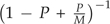times. Assuming that SMARTIE spends nearly all its time computing the likelihood (P→1), in our example above the parallel interface using 12 processors achieves 60% of the theoretical limit, a similar figure to other phylogenetic parallel interfaces (Minh et al. 2005).

In terms of scalability for the number of taxa and the number of nonvertical events, the specific application determines the usefulness of SMARTIE. In theory, SMARTIE should be able to handle any size application, but in practice, as the applications become more complex, the inference does also. These same issues plague much of population genetics research that focuses on recombination rate estimation. In particular, in population genetic applications the size of the model space supported by the data makes inference extremely difficult (Kuhner et al. 2000). In contrast to this, the data in our 2 empirical examples support a much smaller model space, making inference easier. In light of these 2 situations, we avoid giving any precise prescription for scalability, except to say that as the applications become more complex, so does the inference with SMARTIE.

DATA EXAMPLES

We explore a slice of SMARTIE's utility through 2 applications. The first application considers suspected gene conversion among a family of membrane proteins in pathogenic L. interrogans (Stevenson et al. 2007). The data set highlights the feasibility of inference under SMARTIE and demonstrates how phylogenetic data can easily identify a most probable ARG. Our next application illustrates the relationship between SMARTIE and the species-tree concept on the Saccharomyces data set of Rokas et al. (2003).

Leptospira interrogans

Leptospira interrogans are bacterial spirochetes that cause Leptospirosis, an infection primarily of the kidneys and a major cause of human morbidity throughout the developing and developed world. Characterized by severe fever, muscle pain, meningitis, ocular infection, and jaundice, Leptospirosis can progress to systemic infection leading to death due to bleeding of the brain or multiple organ failure (Bharti et al. 2003). Researchers still know little about L. interrogans or its disease mechanism, although progress is underway. One important area under study is the interaction between membrane-bound L. interrogans proteins and human extracellular context. During infection, the L. interrogans protein LenA interacts with several external cellular proteins to avoid host immune response (Verma et al. 2006). Recently, Stevenson et al. (2007) further show that 5 paralogs of the gene lenA, namely lenB, lenC, lenD, lenE, and lenF, produce proteins that interact with the human cellular context to facilitate infection.

In addition to demonstrating these molecular interactions, Stevenson et al. (2007) suggest that the lenF gene in several serovars (lineages) of L. interrogans is actually the product of a nonvertical transmission event and fusion between an ancestral lenC lineage and lenF lineage using the gene-tree methodology of Suchard et al. (2005). Specifically, Stevenson et al. (2007) use a Bayes's factor test to determine whether the lenF lineage forms a monophyletic clade. This test has validity, but an exclusive focus on gene-tree incongruence cannot recover the entire evolutionary history. Consequentially, we reanalyze the molecular sequences from Stevenson et al. (2007) in order to gain a more complete understanding of the history of the paralogs.

The paralogs lenC, lenD, lenE, and lenF each contain 2 distinct motifs, an N-terminal and a C-terminal that arose from a gene duplication event. Because of this duplicity, we break these 4 paralogs into 2 separate gene regions. We also remove the lenB paralog from our data set because strong interlineage variation exists, leaving us with a total of 9 gene regions that we abbreviate as A, CC, CN, DC, DN, EC, EN, FC, and FN. Because these genes are paralogs, we let the operational taxonomic units of our data set represent the N = 9 gene regions and the M = 7 data partitions represent the distinct lineages: Hardjo (har), Grippotyphosa (gri), Canicola (can), Bratislava (bra), Pomona (pom), Copenhageni (cop), and Lai (lai). An alternative representation of these data labels the lineages as the taxa and the paralogs as the partitions. In general, the choice depends upon the application at hand, but this flexibility further identifies a strength of the ARG framework. Back to our problem at hand, we cannot obtain sequence information on the bra lineage for the paralogs DC and DN; this may represent gene loss, so we represent the sequences as standard ambiguity codes, allowing Felsenstein's peeling algorithm to integrate out these 2 sequences when computing the likelihood. We set η = 0.693, implying a 50% prior probability of a nonvertical event before looking at the data. We also consider η = 2, but the results do not notably change. We scale branch lengths in terms of expected substitutions per site and utilize a relatively noninformative gamma prior on the root height. We parameterize Φ under a reassortment prior. To test convergence of our chains, we run 10 independent chains of 15 million iterations with a burn-in of 10%. All 10 chains converge to near identical distributions.

We display the most probable ARG representation of the len family history in Figure 1. Averaging across the independent chains, SMARTIE provides a posterior probability of 89.7% (standard deviation across the 10 chains is 0.3%) for the ARG in Figure 1. Moreover, if we ignore the positioning of paralog DC and “loop-like” nonvertical events (Kuhner et al. 2000) that have no effect on the likelihood, the posterior probability grows well beyond 95%. These “loop-like” events occur when 2 lineages that result from a nonvertical event “coalesce” immediately afterwards. Because of this, these events are essentially hidden and can be safely ignored. Our results with SMARTIE match up with the inferences from Stevenson et al. (2007). Specifically, the lineages gri, pom, bra, and lai derive from an ancestral CN paralog, whereas the other 3 arise from an ancestral F paralog.

Although SMARTIE recovers a single nonvertical event and essentially confirms the results of Stevenson et al. (2007), SMARTIE provides numerous advantages over the previous analysis. Importantly, we gain substantially more information on the evolutionary history. The Bayes's factor test of monophyly in Stevenson et al. (2007) (log₁₀Bf = 8) and a Bayes's factor test of R > 0 versus R = 0 in SMARTIE (log₁₀Bf > 4) recover overwhelming evidence for at least one nonvertical event, but SMARTIE allows us to test for a single event in the history. In particular, testing R = 1 versus R/ = 1, we recover a Bayes's factor of 20 that only a single isolated event occurs in the evolutionary history rather series of nonvertical events. Beyond testing for a single isolated event, use of SMARTIE allows us to date the nonvertical event with a posterior mean of 0.12 and 95% credible interval of (0.06,0.18), with units in expected substitutions per site. If we had simply resorted to testing monophyly, we have no ability to garner this information.

Saccharomyces

This example tackles issues relating ARGs to species-tree inference. Over the past decade, theoretical and applied phylogenetic researchers have recognized that evolutionary histories reconstructed from different genes or loci oftentimes differ from evolutionary histories reconstructed from other locations. Moreover, these gene histories often differ from the presumed organism or species history (Maddison 1997). Acknowledging this phenomenon, researchers have begun to develop methods to better understand this discordance with particular emphasis on estimating species trees (Rannala and Yang 2008).

Initial efforts to reexamine such discordance have focused on the issue of finite data size and quality. Accepting the fact that sequence data provide only a noisy signal for the evolutionary history, many researchers advocate the concatenation of additional sequence data to increase the signal-to-noise ratio, thus better recovering the true species tree (Kluge 1989). Two major successes in this area include Rokas et al. (2003) for Saccharomyces and Chen and Li (2001) for hominid evolution. Simulation work also shows that the concatenation of additional genes or loci allows researchers to narrow in on a single evolutionary history (Rokas and Carroll 2005).

Generally speaking, the addition of more genetic data should allow researchers to narrow in on a single species history, assuming that the underlying statistical model is correct. A vast body of research, however, reveals severe deficiencies in this assumption that can make the addition of more data inappropriate. In statistical terms, the addition of data does not necessarily yield a consistent estimator of the species tree. The most widely studied deficiency of this kind is incomplete lineage sorting (Maddison 1997). Assuming the coalescent model of Kingman (1982), a series of papers demonstrate that the distribution of gene trees resulting from a single species tree exhibits strong variance (Pamilo and Nei 1988; Rosenberg 2002; Degnan and Salter 2005; Kubatko and Degnan 2007) to the point that the most likely gene tree resulting from the species tree may not even coincide with the given species tree (Degnan and Rosenberg 2006). This phenomenon has become so widely recognized that Avise and Robinson (2008) coin the word hemiplasy to describe the situation. The literature contains numerous models to handle this discordance. Liu and Pearl (2007) develop a method to estimate species trees that allows for incomplete lineage sorting in the gene trees and the species tree. Knowles and Carstens (2007) introduce a similar methodology to estimate species trees with a focus on species delimitation. In terms of more general models of discordance, Ané et al. (2007) develop a general approach that clusters gene trees, but their method does not provide further insight into the discordance. Suchard et al. (2005) develop a similar gene-tree procedure that lacks insight into the discordance.

Beyond lineage sorting, little research focuses on other sources of gene-tree incongruence, specifically nonvertical processes. Rokas et al. (2003), Edwards et al. (2007), and Ané et al. (2007) all mention hybridization as a possible explanation for the discordance between gene trees, but the authors do not pursue the ideas to a great degree. In a recent paper comparing methods for species-tree estimation, Linnen and Farrell (2008) further acknowledge that hybridization presents serious problems to the estimation of species trees and that future methods cannot ignore this issue. Linder and Rieseberg (2004) echo similar statements.

We believe that SMARTIE presents an excellent way to incorporate hybridization into the species-tree framework. To explore this idea, we reanalyze the 106 gene Saccharomyces data set of Rokas et al. (2003). We focus our attention on the species Saccharomyces cerevisiae (Scer), Saccharomyces paradoxus (Spar), Saccharomyces mikatae (Smik), Saccharomyces bayanus (Sbay), Saccharomyces kudriavzevii (Skud), and Saccharomyces castellii (Scas). We ignore the 2 other species present in Rokas et al. (2003) as they present a noisier signal. As previously discussed in Rokas et al. (2003) and Edwards et al. (2007), the 106 genes tend to support 1 of 2 evolutionary histories (Fig. 2), with the tree in Figure 2a acting as the most likely species tree (Rokas et al. 2003; Edwards et al. 2007). We note that Rokas et al. (2003) and Edwards et al. (2007) use different underlying evolutionary models, but both label their final estimate as a species tree.

FIGURE 2.

Hybridization in Saccharomyces. Figures (a) and (b) represent the 2 most common gene trees in the Saccharomycesdata set taken from Rokas et al. (2003). The taxa in all 3 figures, Saccharomyces cervevisiae(Scer), Saccharomyces paradoxus(Spar), Saccharomyces mikatae(Smik), Saccharomyces bayanus(Sbay), Saccharomyces kudriavzevii(Skud), and Saccharomyces castellii(Scas), represent distinct species of Saccharomyces. Under SMARTIE, 31 genes on average support the gene tree in (a) and 75 support the gene tree in (b). Because neither bifurcating species history garners overwhelming support, we believe that speciation leading to Sbayand Skudexhibits a strong signal toward hybridization as depicted by the ARG in (c).

We now make inference under SMARTIE. We set η = 0.693 and utilize our Poisson prior on the partition structure with a prior mean of 10% of the number of genes (in this case 10.6) per nonvertical event. We run 10 independent MCMC chains of 3 million iterations. We note that the 10 MCMC chains have difficulty recovering the marginal posterior distribution of the number of nonvertical nodes. This occurs due to strong lineage-specific rate variation in the Scas sequence as compared with the rest of the lineages. SMARTIE attempts to model this variation through nonvertical events that have no effect on the induced tree topologies. Explicitly modeling rate variation in SMARTIE should alleviate such difficulties and remains an important area of active research; we discuss a possible extension in Discussion. Nevertheless, these spurious nonvertical events have no discernable effect on the marginal posterior distribution of the induced gene trees for the 106 loci. In particular, the 10 chains all suggest that 31 genes on average support the tree in Figure 2a and 75 genes support the tree in Figure 2b. Because neither bifurcating species history garners overwhelming support, we believe that speciation leading to Sbay and Skud exhibits a strong signal toward hybridization as depicted by the ARG in Figure 2c. Because of this, a bifurcating species history may not be appropriate for this data set (Liti et al. 2006).

We believe that our analysis using SMARTIE complements and adds to other recent research in this area that explores hybridization. In particular, Meng and Kubatko (2009) allow for hybridization in a species-tree framework, enabling them to tease apart incomplete lineage sorting from hybridization. In their work, however, one needs to specify where the possible hybridization events occur a priori. In a similar work, Than et al. (2007) outline a method to incorporate incomplete lineage sorting but do not discuss how to test for the significance of hybridization events. In both cases, we believe that SMARTIE provides the framework to adequately model and allow for uncertainty in these events. Moreover, the usage of SMARTIE allows investigators the opportunity to formally test the existence of hybridization events.

DISCUSSION

This paper introduces SMARTIE to jointly infer vertical speciation and nonvertical transmission events. Adopting a higher dimensional statistical framework punctuated by an ARG, SMARTIE presents a reasonable and appropriate framework to reconstruct evolutionary histories subject to nonvertical evolution. Moreover, ARGs have widespread use including nonvertical event confirmation, nonvertical event dating, and species delineation.

SMARTIE and its use of ARGs raise numerous statistical modeling issues. We focus here on hierarchical ones. Hierarchical frameworks for phylogenetic data have become quite popular in the past few years (Suchard, Kitchen, et al. 2003; Ané et al. 2007). By pooling information about evolutionary parameters across multilocus data sets, hierarchical frameworks improve statistical power (Gelman et al. 2003) and allow us to gain further insight into evolutionary processes (Huelsenbeck and Suchard 2007; Liang and Weiss 2007). Two specific areas in SMARTIE suggest such a framework. The first involves temporal and lineage-specific rate variation. Over the past decade, investigators have realized the shortcomings of a strict molecular clock (Zuckerkandl and Pauling 1965; Bromham and Penny 2003) and have introduced several models to relax this assumption for bifurcating trees (Thorne et al. 1998; Aris-Brosou and Yang 2002; Drummond et al. 2006). In general, the models allow the infinitesimal rate of character substitution μ(t) to vary over time, with a parameterization dependent upon the tree τ. One possible way to relax the clock of the ARG model is to use the multilocus model of Thorne and Kishino (2002), but because this model does not account for the relationship between 𝒢 and τ, adaptations will be required. This move to a relaxed clock will likely have a significant impact on ARG reconstruction because lineage-specific and temporal rate variation currently confound ARG reconstruction.

The prior we place on the nonvertical partition parameter φ also suggests a hierarchical framework. Back in the Model section of this paper, we introduce 2 priors for φ. Common to them, both the priors assume the independence of each φ_r ∈ φ. In problems where the data suggest low levels of nonvertical evolution, these independent priors make statistical sense. But in problems with high rates of nonvertical evolution, the data strongly suggest a multinomial hierarchical prior. Besides adding statistical power, a hierarchical framework allows for the investigation of the correlation of descent among loci in nonvertical evolution, an idea with implications for selective pressure. For example, a hierarchical prior on an influenza data set allows for the possible grouping of the 8 influenza genes into specific selective classes, an idea that has implications for drug-targeting strategies (Nelson and Holmes 2007).

The above discussion highlights just a few research avenues available through ARGs. In general, most, if not all, research we have previously completed on rooted bifurcating trees can be generalized and extended to ARGs. In fact, this process of abstraction has already begun, for example, the extended Newick format (Cardona et al. 2008) and supernetworks (Holland et al. 2008) have natural analogs in the space of bifurcating trees. To this end, we hope that SMARTIE opens a pathway between the work done in Bayesian phylogenetics and phylogenetic networks. The 2 communities have much to offer each other.

FUNDING

This work was supported by the National Institutes of Health (GM086887, AI07370) and the John Simon Guggenheim Memorial Foundation.

APPENDIX 1

In this section, we provide a method to count the total number of ordered, topologically distinct ARGs with R nonvertical nodes and N external tips. In general, our method adopts a coalescent-like perspective to count the number of ARGs. The recursion starts at current time 0 with N nodes and proceeds backward in time until only one node remains. To start, we define 𝒞 = ( − 1, − 1,…, − 1,1,1,…,1) as the vector of length B = N + 2R − 1 in which the first N + R − 1 positions are equal to − 1 and the remaining R positions are equal to 1. We think of the vector 𝒞 as the left-to-right ordering of the events in an ARG starting at time 0 and moving backward in time toward the root. A − 1 represents a bifurcation event, whereas a 1 represents a nonvertical event. Because every ARG has associated with it 1 permutation of 𝒞, we simply consider the collection of permutations of 𝒞 that correspond to valid ARGs and then count the number of ARGs that correspond to each permutation.

To do this, we first define σ(𝒞) as the set of all unique permutations of 𝒞. For each c ∈ σ(𝒞) and for each i = 1,…,B, we recursively define the function F(c, i) by

(13)

where c_i represents the { − 1,1} value at the ith index of the permutation c. Unfortunately, only specific orderings represent valid ARGs. In particular, only those permutations c ∈ σ(𝒞) that satisfy

(14)

represent valid ARG orderings. The element c_B equals the bth element of c ∈ σ(𝒞). This being the situation, we define the set σ_V(𝒞) ⊂ σ(𝒞) to be those permutations of 𝒞 that satisfy the restrictions in equation (14).

Using this set σ_V(𝒞), we simply need to count the number of ARGs that correspond to each c ∈ σ_V(𝒞) and then sum over all permutations in σ_V(𝒞). In particular, we count the total number of ARGs as

(15)

where I(·) is the indicator function. To unpack this expression, when we encounter a 1 in c, we run into a nonvertical event, of which F(c,i) are possible. When we run into a − 1 or bifurcation event, are possible. Solving equation (15) is computationally expensive. In practice, we use a numerical algorithm to obtain Ω_R,N that adopts a branch-and-bound procedure to limit 𝒞 to σ_V(𝒞).

APPENDIX 2

Here, we describe more fully the 3 MCMC transition kernels we employ in BEAST to make inference through SMARTIE. We only describe the transition kernels novel to our implementation; for details regarding general MCMC theory in phylogenetics, we refer the reader to Larget (2005).

Partition Transition Kernel

This operator acts on the partitioning structure φ. In general, the kernel randomly walks through the partition space Φ in a path dependent on the partition representation. For Φ under a reassortment specification, the kernel goes through 3 steps. First, the kernel uniformly selects a partition φ_r ∈ Φ, then uniformly selects an integer index m in the set {2,3,…,M}, and finally proposes a value φ_rm^☆ = 1 − φ_rm. In more simple language, if φ_rm = 1, the kernel proposes a 0; if φ_rm = 0, the kernel proposes a 1. In the case of a recombination partition space Φ, the kernel uniformly selects a partition φ_r ∈ Φ and then slides the breakpoint of φ_r to left or right dependent upon the flip of a fair coin. Because the kernel acts symmetrically in the reassortment parameterization and recombination parameterization, the Metropolis–Hastings (HM) ratio is the ratio of the posterior under the proposal Θ^☆ to the posterior under the current value Θ. When the kernel proposes partitions outside of Φ, we give the proposal Θ^☆ zero posterior probability.

ARG Swap Kernel

This transition kernel acts on the graph structure 𝒢 using an idea similar to the subtree transfer of standard phylogenetics (Lakner et al. 2008). In reality, this kernel is actually 2 separate kernels, a bifurcation swap and a nonvertical swap. We illustrate both kernels through diagrams in Figure A1; a general mathematical description becomes extremely unwieldy. We start with the bifurcation swap in Figure A1a. To start, the kernel uniformly selects an internal bifurcation node from 𝒢; in the figure, 4 are possible and the kernel selects the one marked with an arrow. After this, the kernel uniformly selects 1 of the 2 children nodes of the selected bifurcation node; in the figure the kernel selects the right child. Next, the kernel breaks the lineages that exist at the time of the selected bifurcation node except the selected child; in the figure, the kernel breaks the lineages marked by the numbers 1, 2, 3, and 4. Finally, the kernel uniformly selects a “swap” lineage. In the figure, the kernel can select among 1, 3, and 4 to “swap” with lineage 2; it chooses lineage 1. Finally, the kernel swaps lineages 1 and 2 and reconnects the graph. Because this kernel is symmetric and acts uniformly at all steps, the HM ratio is the ratio of the posteriors.

FIGURE A1.

ARG swap transition kernel. This figure displays the operations that the ARG swap transition kernel makes. a) The bifurcation swap. In this example, the kernel selects the bifurcation node marked with an arrow and the right lineage of this bifurcation node. Next, the kernel breaks the 4 lineages marked with the numbers 1, 2, 3, and 4. Finally, the kernel swaps lineages 1 and 2 and reattaches the graph as indicated by the dashed lines. The nonvertical swap displayed in (b) acts similarly.

A similar idea works for the nonvertical swap in Figure A1b. First, the kernel uniformly selects 1 of the 2 nonvertical nodes present on the tree; in this case, it selects the one marked with the arrow. Next, the kernel breaks the child lineage of this selected nonvertical node, as well as all others that exist at the time of the nonvertical node. In the figure, the kernel breaks lineages 1, 2, 3, and 4. After this, the kernel uniformly selects a “swap” lineage. In the figure, the kernel can select among 1, 2, and 4; it selects lineage 4. Finally, the kernel “swaps” lineage 3 with lineage 4 and reconnects the graph as shown in Figure A1b. Once again, because this kernel is symmetric and acts uniformly, so the HM ratio equals the ratio of the posteriors.

Reversible Jump Kernel

This final transition kernel adds and removes nonvertical events using the reversible jump methodology of Green (1995). This is the most difficult of the kernels to describe.

To start, the kernel first uniformly selects whether to add a nonvertical node or delete a nonvertical node. If it chooses to add, the kernel then proposes 2 new branch heights from 2 independent exponential distributions with rate parameter α under the restriction that t₁^☆ < t₂^☆ and t₁^☆ < t₀. The parameter t₀ represents the root height of 𝒢. The parameter α is a tuning parameter that we usually set so that p(t₁^☆ < t₀|α) = 0.9. In general, if p₀ equals the probability we choose below the root

(16)

In Figure A2, the kernel draws the heights marked by arrows. After drawing the 2 heights, the kernel then uniformly selects one of the possible lineages at each of the 2 selected heights. At the lower height t₁^☆ in Figure A2, the ARG can choose among 4 lineages (marked with arrows in the upper right figure); at the upper height t₂^☆ in Figure A2, the ARG can select among 5 (not marked). In general, the kernel can select among L(t) lineages at a particular height t. After selecting 2 lineages, the kernel then breaks them, adds a nonvertical node at the lower height t₁^☆, and adds a bifurcation node at the upper height t₂^☆. After this, 2 steps remain. First, the sampler needs to decide whether to attach the first or second parent of the new nonvertical node to the bifurcation node; in the figure, the sampler selects the second or “right” parent. After this, the sampler finishes up by reattaching the remaining lineages and drawing a new partition φ^☆ from p(φ|Φ) to associate with the new nonvertical node.

FIGURE A2.

Reversible jump transition kernel. This figure demonstrates the add step of the reversible jump kernel. First, the kernel draws 2 heights t₁and t₂on G. Next, the kernel uniformly chooses 1 of 4 lineages at t₁(marked with arrows for illustrative purposes) and 1 of 5 lineages at t₂. After selecting the lineages, the kernel adds a bifurcation node onto lineage at t₁and a nonvertical node onto the lineage at t₂. Next, the kernel decides whether to link up the right side or left side of the new nonvertical node to the new bifurcation node; in the figure, the kernel links up the right side of the nonvertical node to the new bifurcation through the dashed line. As a last step, the kernel links up the remaining pieces of the graph.

If t₂^☆ > t₀, the new bifurcation event becomes the new root. Also L(t₂^☆) = 1 when t₂^☆ > t₀. One other small note, if the sampler chooses the same lineage at both heights, we do not include a factor of 2 in the HM ratio because we attach both the first and the second parent of the new nonvertical node to the new bifurcation node. For notational purposes, we let H(L₁^☆,L₂^☆) = 2.0 when the 2 chosen lineages L₁^☆ and L₂^☆ are the same; otherwise H(L₁^☆,L₂^☆) = 1.0.

The delete step of this kernel works as follows. We first find all possible nonvertical nodes that can be deleted. In particular, we find all v_r ∈ 𝒱 such that v_p1(r) and v_p1(r) are not both nonvertical nodes. We let D be the number of nonvertical nodes that satisfy this condition, and we let G(r) = I(v_p1(r)is bifurcation) + I(v_p2(r)is bifurcation) − I(v_p1(r) = v_p2(r)). The subtraction in G(r) is necessary to account for the case when both parents of v_r^☆ are the same. Using these definitions, the kernel first selects a v_r^☆ where G(r) > 0. Next, if G(r) = 2, the kernel selects 1 of the 2 parents of v_r^☆; otherwise, the kernel simply selects the sole bifurcation parent of v_r^☆. Finally, for the parent not selected, the kernel collapses v_r onto this parent and collapses the chosen parent for deletion onto its child. In the process, 𝒢 loses 1 bifurcation node and 1 nonvertical node.

Using the definitions above, the HM ratio for the add step is

(17)

The second term in this ratio accounts for the condition that t₁^☆ < t₂^☆ and t₁^☆ < t₀. The G(r^☆) term represents the function G(·) applied to the just added nonvertical node. The HM ratio for the delete step is the reciprocal of the HM above, with appropriate modifications.

References

- Åkerborg O, Sennblad B, Arvestad L, Lagergren J. Simultaneous Bayesian gene tree reconstruction and reconciliation analysis. Proc. Natl. Acad. Sci. USA. 2009;106:5714–5719. doi: 10.1073/pnas.0806251106. [DOI] [PMC free article] [PubMed] [Google Scholar]
- Altekar G, Dwarkadas S, Huelsenbeck J, Ronquist F. Parallel Metropolis coupled Markov chain Monte Carlo for Bayesian phylogenetic inference. Bioinformatics. 2004;20:407–415. doi: 10.1093/bioinformatics/btg427. [DOI] [PubMed] [Google Scholar]
- Amadal G. AFIPS Conference Proceedings. New York: ACM; 1967. Validity of the single processor approach to achieving large-scale computing capabilities; pp. 483–485. [Google Scholar]
- Andersson J, Sjögren A, Davis L, Embley T, Roger A. Phylogenetic analyses of diplomonad genes reveal frequent lateral gene transfers affecting eukaryotes. Curr. Biol. 2003;13:94–104. doi: 10.1016/s0960-9822(03)00003-4. [DOI] [PubMed] [Google Scholar]
- Ané C, Larget B, Baum D, Smith S, Rokas A. Bayesian estimation of concordance among gene trees. Mol. Biol. Evol. 2007;24:412–426. doi: 10.1093/molbev/msl170. [DOI] [PubMed] [Google Scholar]
- Aris-Brosou S, Yang Z. Effects of models of rate evolution of estimation of divergence dates with special reference to the metazoan 18S ribosomal RNA phylogeny. Syst. Biol. 2002;51:703–714. doi: 10.1080/10635150290102375. [DOI] [PubMed] [Google Scholar]
- Avise J, Robinson T. Hemiplasy: a new term in the lexicon of phylogenetics. Syst. Biol. 2008;57:503–507. doi: 10.1080/10635150802164587. [DOI] [PubMed] [Google Scholar]
- Baroni M, Semple C, Steel M. A framework for representing reticulate evolution. Ann. Combinat. 2004;8:391–408. [Google Scholar]
- Baum D. Concordance trees, concordance factors, and the exploration of reticulate genealogy. Taxon. 2007;56:417–426. [Google Scholar]
- Beiko R, Ragan M. Detecting lateral genetic transfer: a phylogenetic approach. In: Keith J, editor. 2008. Bioinformatics, volume I: data, sequence analysis and evolution. Chapter 21. Methods in Molecular Biology. Totowa (NJ): Humana Press. p. 457–469. [DOI] [PubMed] [Google Scholar]
- Bharti A, Nally J, Ricaldi J, Matthias M, Diaz M, Lovett M, Levett P, Gilman R, Willig M, Gotuzzo E, Vinetz J, Peru-United States Leptospirosis Consortium Leptospirosis: a zoonotic disease of global importance. Lancet Infect. Dis. 2003;3:757–771. doi: 10.1016/s1473-3099(03)00830-2. [DOI] [PubMed] [Google Scholar]
- Bloomquist E, Dorman K, Suchard M. Stepbrothers: inferring partially shared ancestries among recombinant viral sequences. Biostatistics. 2009;10:106–120. doi: 10.1093/biostatistics/kxn019. [DOI] [PMC free article] [PubMed] [Google Scholar]
- Bordewich M, Semple C. Computing the hybridization number of two phylogenetic trees is fixed-parameter tractable. IEEE/ACM Trans. Comput. Biol. Bioinform. 2007;4:458–466. doi: 10.1109/tcbb.2007.1019. [DOI] [PubMed] [Google Scholar]
- Bright R, Shay D, Shu B, Cox N, Klimnov A. Adamantane resistance among influenza A viruses isolated early during the 2005–2006 influenza season in the United States. J. Am. Med. Assoc. 2006;295:891–894. doi: 10.1001/jama.295.8.joc60020. [DOI] [PubMed] [Google Scholar]
- Bromham L, Penny D. The modern molecular clock. Nat. Rev. Genet. 2003;4:216–224. doi: 10.1038/nrg1020. [DOI] [PubMed] [Google Scholar]
- Brown J. Ancient horizontal gene transfer. Nat. Rev. Genet. 2003;4:121–132. doi: 10.1038/nrg1000. [DOI] [PubMed] [Google Scholar]
- Buckley T, Cordeiro M, Marshall D, Simon C. Differentiating between hypotheses of lineage sorting and introgression in New Zealand alpine cicadas. Syst. Biol. 2006;55:411–425. doi: 10.1080/10635150600697283. [DOI] [PubMed] [Google Scholar]
- Cardona G, Rosselló F, Valiente G. Extended Newick: it is time for a standard representation for phylogenetic networks. BMC Bioinformatics. 2008;9:532. doi: 10.1186/1471-2105-9-532. [DOI] [PMC free article] [PubMed] [Google Scholar]
- Chen F, Li W. Genomic divergences between humans and other hominoids and the effective population size of the common ancestor of humans and chimpanzees. Am. J. Hum. Genet. 2001;68:444–456. doi: 10.1086/318206. [DOI] [PMC free article] [PubMed] [Google Scholar]
- Degnan J, Rosenberg N. Discordance of species trees with their most likely gene trees. PLoS. Genet. 2006;2:762–768. doi: 10.1371/journal.pgen.0020068. [DOI] [PMC free article] [PubMed] [Google Scholar]
- Degnan J, Salter L. Gene tree distributions under the coalescent process. Evolution. 2005;59:24–37. [PubMed] [Google Scholar]
- De Iorio M, Griffiths R. Importance sampling on coalescent histories. I. Adv. Appl. Probab. 2004;36:417–433. [Google Scholar]
- Didelot X, Falush D. Inference of bacterial microevolution using multilocus sequence data. Genetics. 2007;175:1251–1266. doi: 10.1534/genetics.106.063305. [DOI] [PMC free article] [PubMed] [Google Scholar]
- Donnelly P, Tavaré S. Coalescents and genealogical structure under neutrality. Annu. Rev. Genet. 1995;29:401–421. doi: 10.1146/annurev.ge.29.120195.002153. [DOI] [PubMed] [Google Scholar]
- Doolittle W. Phylogenetic classification and the universal tree. Science. 1999;284:2124–2129. doi: 10.1126/science.284.5423.2124. [DOI] [PubMed] [Google Scholar]
- Doolittle W, Bapteste E. Pattern pluralism and the tree of life. Proc. Natl. Acad. Sci. USA. 2007;104:2043–2049. doi: 10.1073/pnas.0610699104. [DOI] [PMC free article] [PubMed] [Google Scholar]
- Drummond A, Ho S, Phillips M, Rambaut A. Relaxed phylogenetics and dating with confidence. PLoS Biol. 2006;4:699–710. doi: 10.1371/journal.pbio.0040088. [DOI] [PMC free article] [PubMed] [Google Scholar]
- Drummond A, Rambaut A. BEAST: Bayesian evolutionary analysis by sampling trees. BMC Evol. Biol. 2007;7:214. doi: 10.1186/1471-2148-7-214. [DOI] [PMC free article] [PubMed] [Google Scholar]
- Edwards S, Liu L, Pearl D. High-resolution species trees without concatenation. Proc. Natl. Acad. Sci. USA. 2007;104:5936–5941. doi: 10.1073/pnas.0607004104. [DOI] [PMC free article] [PubMed] [Google Scholar]
- Eldon B, Wakeley J. Coalescent processes when the distribution of offspring number among individuals is highly skewed. Genetics. 2006;172:2621–2633. doi: 10.1534/genetics.105.052175. [DOI] [PMC free article] [PubMed] [Google Scholar]
- Enserink M. A ’wimpy’ flu strain mysteriously turns scary. Science. 2009;323:1162–1163. doi: 10.1126/science.323.5918.1162. [DOI] [PubMed] [Google Scholar]
- Fearnhead P, Donnelly P. Estimating recombination rates from population genetic data. Genetics. 2001;159:1299–1318. doi: 10.1093/genetics/159.3.1299. [DOI] [PMC free article] [PubMed] [Google Scholar]
- Fearnhead P, Donnelly P. Approximate likelihood methods for estimating local recombination rates. J.R. Stat. Soc. B Stat. Methodol. 2002;64:657–680. [Google Scholar]
- Felsenstein J. Evolutionary trees from DNA sequences: a maximum likelihood approach. J. Mol. Evol. 1981;17:368–376. doi: 10.1007/BF01734359. [DOI] [PubMed] [Google Scholar]
- Felsenstein J, Kuhner M, Yamato J, Beerli P. Likelihoods on coalescents: a Monte Carlo sampling approach to inferring parameters from populations samples of molecular data. In: Seillier-Moiseiwitsch F, editor. Statistics in molecular biology. IMS Lecture Notes. Vol. 33. Hayward (CA): Institute of Mathematical Statistics; 1999. pp. 163–184. [Google Scholar]
- Feng X, Buell D, Rose J, Waddell P. Parallel algorithms for Bayesian phylogenetic inference. J. Parallel Distrib. Comput. 2003;63:707–718. [Google Scholar]
- Feng X, Cameron K, Sosa C, Smith B. 2007. Building the tree of life on terascale systems. Parallel and Distributed Processing Symposium. 2007 (IPDPS 2007). Piscataway (NJ): IEEE. [Google Scholar]
- Fisher R. The genetical theory of natural selection. Oxford: Clarendon Press; 1930. [Google Scholar]
- Fu Y. Exact coalescent for the Wright-Fisher model. Theor. Popul. Biol. 2006;69:385–394. doi: 10.1016/j.tpb.2005.11.005. [DOI] [PubMed] [Google Scholar]
- Gelman A, Carlin J, Stern H, Rubin D. Bayesian data analysis. 2nd ed. New York: Chapman and Hall; 2003. [Google Scholar]
- Gladyshev E, Meselson M, Arkhipova I. Massive horizontal gene transfer in bdelloid rotifers. Science. 2008;320:1210–1213. doi: 10.1126/science.1156407. [DOI] [PubMed] [Google Scholar]
- Grassly N, Holmes E. A likelihood method for the detection of selection and recombination using nucleotide sequences. Mol. Biol. Evol. 1997;14:239–247. doi: 10.1093/oxfordjournals.molbev.a025760. [DOI] [PubMed] [Google Scholar]
- Green P. Reversible jump Markov chain Monte Carlo computation and Bayesian model determination. Biometrika. 1995;82:711–732. [Google Scholar]
- Griffiths R, Jenkins P, Song Y. Importance sampling and the two-locus model with subdivided population structure. Adv. Appl. Probab. 2008;40:473–500. doi: 10.1239/aap/1214950213. [DOI] [PMC free article] [PubMed] [Google Scholar]
- Griffiths R, Marjoram P. Ancestral inference from samples of DNA sequences with recombination. J. Comput. Biol. 1996;3:479–502. doi: 10.1089/cmb.1996.3.479. [DOI] [PubMed] [Google Scholar]
- Gusfield D, Eddhu S, Langley C. Optimal, efficient reconstruction of phylogenetic networks with constrained recombination. J Bioinform. Comput. Biol. 2004;2:173–214. doi: 10.1142/s0219720004000521. [DOI] [PubMed] [Google Scholar]
- Hasegawa M, Kishino H, Yano T. Dating the human-ape splitting by a molecular clock of mitochondrial DNA. J. Mol. Evol. 1985;22:160–174. doi: 10.1007/BF02101694. [DOI] [PubMed] [Google Scholar]
- Hein J. A heuristic method to reconstruct the history of sequences subject to recombination. J. Mol. Evol. 1993;36:396–405. [Google Scholar]
- Holland B, Benthin S, Lockhart P, Moulton V, Huber K. Using supernetworks to distinguish hybridization from lineage-sorting. BMC Evol. Biol. 2008;8:202. doi: 10.1186/1471-2148-8-202. [DOI] [PMC free article] [PubMed] [Google Scholar]
- Hudson R. Properties of a neutral allele model with intragenic recombination. Theor. Popul. Biol. 1983;23:183–201. doi: 10.1016/0040-5809(83)90013-8. [DOI] [PubMed] [Google Scholar]
- Hudson R. Two-locus sampling distributions and their application. Genetics. 2001;159:1805–1817. doi: 10.1093/genetics/159.4.1805. [DOI] [PMC free article] [PubMed] [Google Scholar]
- Hudson R, Kaplan N. Statistical properties of the number of recombination events in the history of a sample. Genetics. 1985;111:147–164. doi: 10.1093/genetics/111.1.147. [DOI] [PMC free article] [PubMed] [Google Scholar]
- Huelsenbeck J, Suchard M. A nonparametric method for accommodating and testing across-site rate variation. Syst. Biol. 2007;56:975–987. doi: 10.1080/10635150701670569. [DOI] [PubMed] [Google Scholar]
- Husmeier D, McGuire G. Detecting recombination in 4-taxa DNA sequence alignments with Bayesian hidden Markov models and Markov chain Monte Carlo. Mol. Biol. Evol. 2003;20:315–337. doi: 10.1093/molbev/msg039. [DOI] [PubMed] [Google Scholar]
- Huson D, Bryant D. Application of phylogenetic networks in evolutionary studies. Mol. Biol. Evol. 2006;23:254–267. doi: 10.1093/molbev/msj030. [DOI] [PubMed] [Google Scholar]
- Jin G, Nakhleh L, Snir S, Tuller T. Maximum likelihood of phylogenetic networks. Bioinformatics. 2006;22:2604–2611. doi: 10.1093/bioinformatics/btl452. [DOI] [PubMed] [Google Scholar]
- Jin G, Nakhleh L, Snir S, Tuller T. Inferring phylogenetic networks by the maximum parsimony criterion: a case study. Mol. Biol. Evol. 2007;24:324–337. doi: 10.1093/molbev/msl163. [DOI] [PubMed] [Google Scholar]
- Keane T, Naughton T, Travers S, McInerney J, McCormack G. DPRml: distributed phylogeny reconstruction by maximum likelihood. Bioinformatics. 2005;21:969–974. doi: 10.1093/bioinformatics/bti100. [DOI] [PubMed] [Google Scholar]
- Kingman J. On the genealogy of large populations. J. Appl. Probab. 1982;19:27–43. [Google Scholar]
- Kluge A. A concern for evidence and a phylogenetic hypothesis of relationships among Epicrates (Boidae,Serpentes) Syst. Zool. 1989;38:7–25. [Google Scholar]
- Knowles L, Carstens B. Delimiting species without monophyletic gene trees. Syst. Biol. 2007;56:887–895. doi: 10.1080/10635150701701091. [DOI] [PubMed] [Google Scholar]
- Koonin E. Darwinian evolution in the light of genomics. Nucleic Acids. Res. 2009;37:1011–1034. doi: 10.1093/nar/gkp089. [DOI] [PMC free article] [PubMed] [Google Scholar]
- Kubatko L, Degnan J. Inconsistency of phylogenetic estimates from concatenated data under coalescence. Syst. Biol. 2007;56:17–24. doi: 10.1080/10635150601146041. [DOI] [PubMed] [Google Scholar]
- Kuhner M, Yamato J, Felsenstein J. Maximum likelihood estimation of recombination rates from population data. Genetics. 2000;156:1393–1401. doi: 10.1093/genetics/156.3.1393. [DOI] [PMC free article] [PubMed] [Google Scholar]
- Lakner C, van der Mark P, Huelsenbeck J, Larget B, Ronquist F. Efficiency of Markov chain Monte Carlo tree proposals in Bayesian phylogenetics. Syst. Biol. 2008;57:86–103. doi: 10.1080/10635150801886156. [DOI] [PubMed] [Google Scholar]
- Larget B. Introduction to Markov chain Monte Carlo methods in molecular evolution. In: Nielsen R, editor. Statistical methods in molecular evolution. New York: Springer; 2005. pp. 45–62. [Google Scholar]
- Lawrence J, Ochman H. Molecular archaeology of the Escherichia coli genome. Proc. Natl. Acad. Sci. USA. 1998;95:9413–9417. doi: 10.1073/pnas.95.16.9413. [DOI] [PMC free article] [PubMed] [Google Scholar]
- Leverstein-van Hall M, Box A, Block H, Paauw A, Fluit A, Verhoef J. Evidence of extensive interspecies transfer of integron-mediated antimicrobial resistance genes among multidrug-resistant Enterobacteriaceae in a clinical setting. J. Infect. Dis. 2002;186:49–56. doi: 10.1086/341078. [DOI] [PubMed] [Google Scholar]
- Li N, Stephens M. Modeling linkage disequilibrium and identifying recombination hotspots using single-nucleotide polymorphism data. Genetics. 2003;165:2213–2233. doi: 10.1093/genetics/165.4.2213. [DOI] [PMC free article] [PubMed] [Google Scholar]
- Li S, Pearl D, Doss H. Phylogenetic tree construction using Markov chain Monte Carlo. J. Am. Stat. Assoc. 2000;95:493–508. [Google Scholar]
- Liang L, Weiss R. A hierarchical semiparametric regression model for combining HIV-1 phylogenetic analyses using iterative reweighting algorithms. Biometrics. 2007;63:733–741. doi: 10.1111/j.1541-0420.2007.00753.x. [DOI] [PubMed] [Google Scholar]
- Linder C, Rieseberg L. Reconstructing patterns of reticulate evolution in plants. Am. J. Bot. 2004;91:1700–1708. [PMC free article] [PubMed] [Google Scholar]
- Lindstrom S, Cox N, Klimov A. Genetic analysis of human H2N2 and early H3N2 influenza viruses, 1957–1972: evidence for genetic divergence and multiple reassortment events. Virology. 2004;328:101–119. doi: 10.1016/j.virol.2004.06.009. [DOI] [PubMed] [Google Scholar]
- Linnen C, Farrell B. Comparison of methods for species-tree inference in the sawfly genus Neodiprion (Hymenoptera:Diprionidae) Syst. Biol. 2008;57:876–890. doi: 10.1080/10635150802580949. [DOI] [PubMed] [Google Scholar]
- Liti G, Barton D, Lewis E. Sequence diversity, reproductive isolation and species concepts in Saccharomyces. Genetics. 2006;174:839–850. doi: 10.1534/genetics.106.062166. [DOI] [PMC free article] [PubMed] [Google Scholar]
- Liu J. Monte Carlo strategies in scientific computing. New York: Springer; 2001. [Google Scholar]
- Liu L, Pearl D. Species trees from gene trees: reconstructing Bayesian posterior distributions of a species phylogeny using estimated gene tree distributions. Syst. Biol. 2007;56:504–514. doi: 10.1080/10635150701429982. [DOI] [PubMed] [Google Scholar]
- Lyngsø R, Song Y, Hein J. 2008. Accurate computation of likelihoods in the coalescent with recombination via parsimony. Proceedings of the 12th Annual International Conference on Research in Computational Molecular Biology (RECOMB 2008). Berlin: Springer. [Google Scholar]
- Maddison W. Gene trees in species trees. Syst. Biol. 1997;46:523–536. [Google Scholar]
- Mallet J. Hybrid speciation. Nature. 2007;446:279–283. doi: 10.1038/nature05706. [DOI] [PubMed] [Google Scholar]
- McVean G, Cardin N. Approximating the coalescent with recombination. Philos. Trans. Biol. Sci. 2005;360:1387–1393. doi: 10.1098/rstb.2005.1673. [DOI] [PMC free article] [PubMed] [Google Scholar]
- McVean G, Myers S, Hunt S, Deloukas P, Bentley D, Donnelly P. The fine-scale structure of recombination rate variation in the human genome. Science. 2004;304:581–584. doi: 10.1126/science.1092500. [DOI] [PubMed] [Google Scholar]
- Meng C, Kubatko L. Detecting hybrid speciation in the presence of incomplete lineage sorting using gene tree incongruence: a model. Theor. Popul. Biol. 2009;75:35–45. doi: 10.1016/j.tpb.2008.10.004. [DOI] [PubMed] [Google Scholar]
- Minh B, Vinh L, von Haeseler A, Schmidt H. pIQPNNI: parallel reconstruction of large maximum likelihood phylogenies. Bioinformatics. 2005;21:3794–3796. doi: 10.1093/bioinformatics/bti594. [DOI] [PubMed] [Google Scholar]
- Minin V, Dorman K, Fang F, Suchard M. Dual multiple change-point model leads to more accurate recombination detection. Bioinformatics. 2005;21:3034–3042. doi: 10.1093/bioinformatics/bti459. [DOI] [PubMed] [Google Scholar]
- Moran P. A general theory of the distribution of gene frequencies I. Overlapping generations. Proc. R. Soc. Lond. B Biol. Sci. 1958;149:102–112. doi: 10.1098/rspb.1958.0054. [DOI] [PubMed] [Google Scholar]
- Moret B, Bader D, Warnow T. High-performance algorithm engineering for computational phylogenetics. J. Supercomput. 2002;22:99–111. [Google Scholar]
- Myers S, Bottolo L, Freeman C, McVean G, Donnelly P. A fine-scale map of recombination rates and hotspots across the human genome. Science. 2005;310:321–324. doi: 10.1126/science.1117196. [DOI] [PubMed] [Google Scholar]
- Nelson K, Clayton R, Gill S, Gwinn M, Dodson R, Haft D, Hickey E, Peterson J, Nelson W, Ketchum K, McDonald L, Utterback T, Malek J, Linher K, Garrett M, Stewart A, Cotton M, Pratt M, Phillips C, Richardson D, Heidelberg J, Sutton G, Fleischmann R, Eisen J, White O, Salzberg S, Smith H, Venter J, Fraser C. Evidence for lateral gene transfer between Archaea and bacteria from genome sequence of Thermotoga maritima. Nature. 1999;399:323–329. doi: 10.1038/20601. [DOI] [PubMed] [Google Scholar]
- Nelson M, Holmes E. The evolution of epidemic influenza. Nat. Rev. Genet. 2007;8:196–205. doi: 10.1038/nrg2053. [DOI] [PubMed] [Google Scholar]
- Nielsen R. Estimation of population parameters and recombination rates from single nucleotide polymorphisms. Genetics. 2000;154:931–942. doi: 10.1093/genetics/154.2.931. [DOI] [PMC free article] [PubMed] [Google Scholar]
- Nora T, Charpentier C, Tenaillon O, Hoede C, Clavel F, Hance A. Contribution of recombination to the evolution of human immunodeficiency viruses expressing resistance to antiretroviral treatment. J. Virol. 2007;81:7620–7628. doi: 10.1128/JVI.00083-07. [DOI] [PMC free article] [PubMed] [Google Scholar]
- Pamilo P, Nei M. Relationships between gene trees and species trees. Mol. Biol. Evol. 1988;5:568–583. doi: 10.1093/oxfordjournals.molbev.a040517. [DOI] [PubMed] [Google Scholar]
- Philippe H, Delsuc F, Brinkmann H, Lartillot N. Phylogenomics. Annu. Rev. Ecol. Syst. 2005;36:541–562. [Google Scholar]
- Posada D, Crandall K, Holmes E. Recombination in evolutionary genomics. Annu. Rev. Genet. 2002;36:75–97. doi: 10.1146/annurev.genet.36.040202.111115. [DOI] [PubMed] [Google Scholar]
- Rambaut A, Posada D, Crandall K, Holmes E. The causes and consequences of HIV evolution. Nat. Rev. Genet. 2004;5:52–61. doi: 10.1038/nrg1246. [DOI] [PubMed] [Google Scholar]
- Rannala B, Yang Z. Phylogenetic inference using whole genomes. Annu. Rev. Genomics Hum. Genet. 2008;9:17–31. doi: 10.1146/annurev.genom.9.081307.164407. [DOI] [PubMed] [Google Scholar]
- Richardson A, Palmer J. Horizontal gene transfer in plants. J. Exp. Bot. 2007;58:1–9. doi: 10.1093/jxb/erl148. [DOI] [PubMed] [Google Scholar]
- Rokas A, Carroll S. More genes or more taxa? The relative contribution of gene number and taxon number to phylogenetic accuracy. Mol. Biol. Evol. 2005;22:1337–1344. doi: 10.1093/molbev/msi121. [DOI] [PubMed] [Google Scholar]
- Rokas A, Williams B, King N, Carroll S. Genome-scale approaches to resolving incongruence in molecular phylogenies. Nature. 2003;425:798–804. doi: 10.1038/nature02053. [DOI] [PubMed] [Google Scholar]
- Rosenberg N. The probability of topological concordance of gene trees and species trees. Theor. Popul. Biol. 2002;61:225–247. doi: 10.1006/tpbi.2001.1568. [DOI] [PubMed] [Google Scholar]
- Schmidt H, Strimmer K, Vingron M, von Haeseler A. TREE-PUZZLE: maximum likelihood phylogenetic analysis using quartets and parallel computing. Bioinformatics. 2002;18:502–504. doi: 10.1093/bioinformatics/18.3.502. [DOI] [PubMed] [Google Scholar]
- Simonsen L, Viboud C, Grenfell B, Dushoff J, Jennings L, Smit M, Macken C, Hata M, Gog J, Miller M, Holmes E. The genesis and spread of reassortment human influenza A/H3N2 viruses conferring Adamantane resistance. Mol. Biol. Evol. 2007;24:1811–1820. doi: 10.1093/molbev/msm103. [DOI] [PubMed] [Google Scholar]
- Song Y, Hein J. Constructing minimal ancestral recombination graphs. J. Comput. Biol. 2005;12:147–169. doi: 10.1089/cmb.2005.12.147. [DOI] [PubMed] [Google Scholar]
- Stamatakis A, Ludwig T, Meier H. Parallel inference of a 10,000-taxon phylogeny with maximum likelihood. In: Danelutto M, Laforenza D, Vanneschi M, editors. Euro-Par 2004 Parallel Processing. Lecture Notes in Computer Science. Vol. 3149. Berlin: Springer; 2004. pp. 997–1004. [Google Scholar]
- Stamatakis A, Ludwig T, Meier H. RAxML-III: a fast program for maximum likelihood-based inference of large phylogenetic trees. Bioinformatics. 2005;21:456–463. doi: 10.1093/bioinformatics/bti191. [DOI] [PubMed] [Google Scholar]
- Stephens M, Donnelly P. Inference in molecular population genetics. J.R. Stat. Soc. B Stat. Methodol. 2000;62:605–655. [Google Scholar]
- Stevenson B, Choy H, Pinne M, Rotondi M, Miller M, DeMoll E, Kraiczy P, Cooley A, Creamer T, Suchard M, Brissette C, Verma A, Haake D. Leptospira interrogans endostatin-like outer membrane proteins bind host fibronectin, laminin and regulators of complement. PLoS One. 2007;2:e1188. doi: 10.1371/journal.pone.0001188. [DOI] [PMC free article] [PubMed] [Google Scholar]
- Stewart C, Hart D, Berry D, Olsen G, Wernet E, Fischer W. Proceedings of the Supercomputing Conference (SC2001) Denver, CO. New York: ACM; 2001. Parallel implementation and performance of fastDNAml—a program for maximum likelihood phylogenetic inference. [Google Scholar]
- Strimmer K, Wiuf C, Moulton V. Recombination analysis using directed graphical models. Mol. Biol. Evol. 2001;18:97–99. doi: 10.1093/oxfordjournals.molbev.a003725. [DOI] [PubMed] [Google Scholar]
- Stumpf M, McVean G. Estimating recombination rates from population-genetic data. Nat. Rev. Genet. 2003;4:363–370. doi: 10.1038/nrg1227. [DOI] [PubMed] [Google Scholar]
- Suchard M, Kitchen C, Sinsheimer J, Weiss R. Hierarchical phylogenetic models for analyzing multipartite sequence data. Syst. Biol. 2003;52:649–664. doi: 10.1080/10635150390238879. [DOI] [PubMed] [Google Scholar]
- Suchard M, Rambaut A. Many-core algorithms for statistical phylogenetics. Bioinformatics. 2009;25:1370–1376. doi: 10.1093/bioinformatics/btp244. [DOI] [PMC free article] [PubMed] [Google Scholar]
- Suchard M, Weiss R, Dorman K, Sinsheimer J. Inferring spatial phylogenetic variation along nucleotide sequences: a multiple changepoint model. J. Am. Stat. Assoc. 2003;98:427–437. [Google Scholar]
- Suchard M, Weiss R, Sinsheimer J. Models for estimating Bayes factors with applications to phylogeny and tests of monophyly. Biometrics. 2005;61:665–673. doi: 10.1111/j.1541-0420.2005.00352.x. [DOI] [PubMed] [Google Scholar]
- Temin H. Sex and recombination in retroviruses. Trends Genet. 1991;7:71–74. doi: 10.1016/0168-9525(91)90272-R. [DOI] [PubMed] [Google Scholar]
- Than C, Ruths D, Innan H, Nakhleh L. Confounding factors in HGT detection: statistical error, coalescent effects, and multiple solutions. J. Comput. Biol. 2007;14:517–535. doi: 10.1089/cmb.2007.A010. [DOI] [PubMed] [Google Scholar]
- Thorne J, Kishino H. Divergence time and evolutionary rate estimation with multilocus data. Syst. Biol. 2002;51:689–702. doi: 10.1080/10635150290102456. [DOI] [PubMed] [Google Scholar]
- Thorne J, Kishino H, Painter I. Estimating the rate of evolution of the rate of molecular evolution. Mol. Biol. Evol. 1998;15:1647–1657. doi: 10.1093/oxfordjournals.molbev.a025892. [DOI] [PubMed] [Google Scholar]
- Verma A, Hellwage J, Artiushin S, Zipfel P, Kraiczy P, Timoney J, Stevenson B. LfhA, a novel factor H-binding protein of Leptospira interrogans. Infect. Immun. 2006;74:2659–2666. doi: 10.1128/IAI.74.5.2659-2666.2006. [DOI] [PMC free article] [PubMed] [Google Scholar]
- Wakeley J. The limits of theoretical population genetics. Genetics. 2005;169:1–7. doi: 10.1093/genetics/169.1.1. [DOI] [PMC free article] [PubMed] [Google Scholar]
- Wall J. A comparison of estimators of the population recombination rate. Mol. Biol. Evol. 2000;17:156–163. doi: 10.1093/oxfordjournals.molbev.a026228. [DOI] [PubMed] [Google Scholar]
- Wang L, Zhang K, Zhang L. Perfect phylogenetic networks with recombination. J. Comput. Biol. 2001;8:69–78. doi: 10.1089/106652701300099119. [DOI] [PubMed] [Google Scholar]
- Wang Y, Rannala B. Bayesian inference of fine-scale recombination rates using population genomic data. Philos. Trans. R. Soc. Lond. B Biol. Sci. 2008;363:3921–3930. doi: 10.1098/rstb.2008.0172. [DOI] [PMC free article] [PubMed] [Google Scholar]
- Wilson D, Gabriel E, Leatherbarrow A, Cheesbrough J, Gee S, Bolton E, Fox A, Hart C, Diggle P, Fearnheard P. Rapid evolution and the importance of recombination to the gastroenteric pathogen Campylobacter jejuni. Mol. Biol. Evol. 2009;26:385–397. doi: 10.1093/molbev/msn264. [DOI] [PMC free article] [PubMed] [Google Scholar]
- Winckler W, Myers S, Richter D, Onofrio R, McDonald G, Bontrop R, McVean G, Reich SGD, Donnelly P, Altshuler D. Comparison of the fine-scale recombination rates in humans and chimpanzees. Science. 2005;308:107–111. doi: 10.1126/science.1105322. [DOI] [PubMed] [Google Scholar]
- Wolf Y, Rogozin I, Grishin N, Koonin E. Genome trees and the tree of life. Trends Genet. 2002;18:472–479. doi: 10.1016/s0168-9525(02)02744-0. [DOI] [PubMed] [Google Scholar]
- Woolley S, Posada D, Crandall K. A comparison of phylogenetic network methods using computer simulation. Plos One. 2008;3:e1913. doi: 10.1371/journal.pone.0001913. [DOI] [PMC free article] [PubMed] [Google Scholar]
- Wright S. Evolution in Mendelian populations. Genetics. 1931;16:97–159. doi: 10.1093/genetics/16.2.97. [DOI] [PMC free article] [PubMed] [Google Scholar]
- Wu Q, James S, Roberts I, Moulton V, Huber K. Exploring contradictory phylogenetic relationships in yeasts. FEMS Yeast Res. 2008;8:641–650. doi: 10.1111/j.1567-1364.2008.00362.x. [DOI] [PubMed] [Google Scholar]
- Yang Z. Maximum likelihood phylogenetic estimation from DNA sequences with variable rates over sites: approximate methods. J. Mol. Evol. 1994;39:306–314. doi: 10.1007/BF00160154. [DOI] [PubMed] [Google Scholar]
- Zhou B, Jermiin L. 2004. Parallel implementation of maximum likelihood methods for phylogenetic analysis. 18th International Parallel and Distributed Processing Symposium (IPDPS'04). Amsterdam: Elsevier. [Google Scholar]
- Zuckerkandl E, Pauling L. Evolutionary divergence and convergence in proteins. In: Bryson V, Vogel H, editors. Evolving genes and proteins. New York: Academic Press; 1965. pp. 97–166. [Google Scholar]