Improving PET receptor binding estimates from Logan plots using principal component analysis

Abstract

This work reports a principal component analysis (PCA)-based approach for reducing bias in distribution volume ratio (DVR) estimates from Logan plots in positron emission tomography (PET). Comparison has been made of all existing bias-removal methods with the proposed PCA method, for both single-estimate PET studies and intervention studies where pre- and post-intervention estimates are made. Bias in Logan-based DVR estimates is because of the noise in the PET time-activity curves (TACs) that propagates as correlated errors in dependent and independent variables of the Logan equation. Intervention studies show this same bias but also higher variance in DVR estimates. In this work, noise in the TACs was reduced by fitting the curves to a low-dimension PCA-based linear model, leading to reduced bias and variance in DVR. For validating the approach, TACs with realistic noise were simulated for a ¹¹C-labeled tracer with carfentanil (CFN)-like kinetics for both single-measurement and intervention studies. Principal component analysis and existing methods were applied to the simulated data and their performance was compared by statistical analysis. The results indicated that existing methods either removed only part of the bias or reduced bias at the expense of precision. The proposed method removed ∼90% of the bias while also improving precision in both single- and dual-measurement simulations. After validation of the proposed method in simulations, PCA, along with the existing methods, was applied to human [¹¹C]CFN data acquired for both single estimation of DVR and dual-estimation intervention studies. Similar results were observed in human scans as were seen in the simulation studies.

Introduction

For most positron emission tomography (PET) radiotracers, the tracer concentration time course in brain can be modeled as a nonlinear function of rate parameters of a chosen pharmacokinetic model (Carson, 1986). These kinetic parameters are estimated by fitting the dynamic PET data to the kinetic model, using nonlinear estimation techniques. The distribution volume ratio (DVR), a popular index of receptor binding site density related to the non-displaceable binding potential (BP_ND), is a function of these rate parameters. Nonlinear estimation techniques are computationally expensive, and under noisy conditions may not converge, thus reducing viability for voxel-by-voxel parametric image generation. Logan plot analysis, a computationally efficient alternative, has been proposed for reversible tracers, where ordinary least squares (OLS) can be used to estimate DVR after transformation of dynamic PET data (Logan et al, 1996). Logan plot analysis has been used extensively because of its simplicity and model independence. However, negative bias exists in Logan plot-based DVR estimates, owing to the noise present in time activity curves (TACs) that propagates as correlated errors in the dependent and independent variables of the Logan plot equation (Slifstein and Laruelle, 2000). We have found that this noise propagation is more pronounced (resulting in higher bias and variance) in PET studies that involve a pharmacological or behavioral intervention, primarily because of the restricted temporal range of data available for DVR estimation. In these studies, two pharmacokinetic measurements are obtained from a single-tracer injection, before and after the intervention. It is important to have a method to reduce bias as well as maintain high precision in the parameter estimates from such experiments.

To reduce the bias in single-measurement PET studies, various methods have been proposed previously for the arterial sampling approach (Logan et al, 2001; Varga and Szabo, 2002; Ichise et al, 2002; Ogden, 2001). The operational Logan plot equations for both arterial sampling and reference region approaches have the same problem of correlated errors in both dependent and independent variables. The references mentioned above address this problem of correlated errors and hence should be applicable to both arterial sampling and reference region approaches. We found that these existing methods either removed the bias at the expense of precision or removed only part of the bias. In this paper, we introduce a new approach for reducing bias using principal component analysis (PCA), which is a feature extraction technique used to simplify a data set by reducing its dimensionality while maintaining its relevant characteristics. Principal component analysis has been used extensively in nuclear imaging, including PET, in the spatial domain (Barber, 1980; Pedersen et al, 1994; Thireou et al, 2003; Razifar et al, 2006), where the investigators have analyzed the images of the coefficients of individual principal components. Principal component analysis has been previously used in temporal domain in PET for clustering the TACs before parameter estimation (Kimura et al, 2002) and separation of TACs in dual-tracer scans (Kadrmas and Rust, 2005). Frequency analysis of dynamic structures, where the principal components are rotated to avoid negative values, has been used in temporal domain in single photon emission computed tomography (Sitek et al, 1999). In this work, we apply PCA to achieve temporal smoothing of PET TACs to reduce the bias in DVR estimates.

Theoretical background

The differential equations for a two tissue compartment model for a PET tracer are shown below:

$$\frac{\text{d}{C}_{\text{ND}}(t)}{\text{d}t}=K_1{C}_{\text{p}}(t)-(k_2+k_3)C_{\text{ND}}(t)+k_4{C}_{\text{S}}(t)$$ (1)

$$\frac{\text{d}{C}_{\text{S}}(t)}{\text{d}t}=k_3{C}_{\text{ND}}(t)-k_4{C}_{\text{S}}(t)$$ (2)

where C_p(t) is the arterial plasma input, C_ND(t) is the radioligand concentration in the nondisplaceable compartment, C_S(t) is the radioligand concentration in the specific compartment, and K₁, k₂, k₃, and k₄ are the kinetic parameters of the model. The total concentration of the radioligand in the tissue is given by

$$C_{\text{T}}(t)=C_{\text{ND}}(t)+C_{\text{S}}(t)=C_{\text{p}}(t)\otimes \text{IR}(t)$$ (3)

where IR(t) is the tissue impulse response and is the sum of two exponential terms as shown below:

$$\text{IR}(t)={A_1\text{e}}^{-{\alpha }_{1}t}+{A_2\text{e}}^{-{\alpha }_{2}t}$$ (4)

with α₁, α₂, A₁, and A₂ being combinations of the individual rate parameters, K₁ to k₄.

The non-displaceable binding potential (BP_ND), a commonly used index of receptor binding density, is the ratio of the equilibrium concentration of specifically bound to nondisplaceable radioligand in any given region (k₃/k₄). Direct estimation of BP_ND from equations (3) and (4) suffers from the practical difficulties of arterial blood sampling and the possible errors associated with it, as well as being computationally expensive because of the nature of nonlinear estimation techniques. Conversely, the reference region approach proposed by Logan et al (1996) avoids arterial sampling by using a region assumed to be devoid of specific binding sites to estimate a similar index of binding termed DVR (= BP_ND + 1).

In the reference region-based Logan plot approach, DVR is estimated using OLS by transformation of the dynamic PET data as shown below:

$$\frac{{\int }_0^{T_i}{C}_{\text{T}}(t)\text{d}t}{C_{\text{T}}(T_i)}=\mathit{\text{DVR}}\frac{{\int }_0^{T_i}{C}_{\text{ref}}(t)\text{d}t+\left(C_{\text{ref}}(T_i)/k_2^{\text{ref}}\right)}{C_{\text{T}}(T_i)}+\mathit{\text{INT}}$$ (5)

where INT is an intercept term, T_i is the midpoint time of the ith frame, and $k_2^{\text{ref}}$ is the chosen k₂ parameter for the reference region. Equation (5) becomes linear over multiple time measurements of the target and reference tissues after time T′, and DVR is estimated by calculating the slope of the line. The numerators in both the dependent variable

$$\frac{\underset{0}{\overset{T_i}{\int }}{C}_{\text{T}}(t)\text{d}t}{C_{\text{T}}(T_i)}$$

and independent variable

$$\frac{\underset{0}{\overset{T_i}{\int }}{C}_{\text{ref}}(t)\text{d}t+\frac{C_{\text{ref}}(T_i)}{k_2^{\text{ref}}}}{C_{\text{T}}(T_i)}$$

have integral terms and are relatively noise free as compared with the denominators. It has been reported that the presence of the noisy term (C_T(T_i)) in the denominators on both sides of equation (5) is the cause of correlated errors leading to negative bias in DVR estimates (Slifstein and Laruelle, 2000). This bias is more pronounced in regions with higher DVR values. Reduction of noise in the measured TACs will assist in reducing the correlated errors leading to a reduction in the bias. In this work, we propose a PCA-based approach to achieve this.

PET Studies with Pharmacological Intervention

A pharmacological intervention study involves obtaining two measures of one neuropharmacological parameter from a single PET study. A single tracer is administered, and at some point during the PET data acquisition, an interventional challenge or perturbation of the system is made with the intent of changing in vivo distribution of the radiotracer. Logan plots are used to estimate DVR before and after intervention (Koeppe, 2002). The bias and variance is more pronounced in this case because fewer data points are available for DVR estimation compared to when a single measurement is made. Application of the existing bias-removal techniques to such intervention studies has not been reported in the literature. Except for the temporal range of data used, the procedure for estimating DVR in intervention and single-measurement studies is the same. The Logan plots for dual-measurement intervention studies have the same noise-induced bias associated with them as in single-measurement studies. Thus, although the existing methods have been proposed for single-measurement studies, they should be applicable to the dual-Logan case without any modifications. We applied the proposed PCA-based approach as well as the existing methods to reduce the bias in PET intervention studies (both simulations and human studies).

Materials and methods

Principal Component Analysis

Principal component analysis is a feature extraction technique used to simplify a data set by reducing its dimensionality while maintaining its important characteristics (Faraway, 2004). In feature extraction, data space is transformed into a ‘feature’ space having the same dimensions as the data set. This transformation is such that the data set can then be represented by a reduced number of dominant ‘features’ while retaining all the important intrinsic characteristics of the original data. Using PCA, each original data vector of dimension ‘p’ can be expressed as a linear combination of ‘p’ orthogonal basis vectors. By limiting the number of basis vectors to ‘q’ dominant vectors (q<p), data can be represented with a reduced dimensionality, thus reducing the noise and preserving all the important features in the data. Using PCA, the noise in the PET TAC values (C_T(T_i)) can be reduced, thus reducing the correlated errors in equation (5), which is the cause of bias in DVR estimates.

The classical model for a PET TAC is a nonlinear function of rate parameters (equations (3) and (4)). Here, we represented dynamic PET data using a PCA-based linear model. Thus, a noisy tissue curve vector for the jth voxel, ȳ_j = [C_Tj(T₁), C_Tj(T₂),⋯, C_Tj (T_p)]′ ∈ R^p×1, from a PET study involving ‘p’ temporal frames can be expressed as

$${\overline{y}}_j=G{\overline{x}}_j+{\overline{\epsilon }}_j$$ (6)

where G∈R^p×q is the system matrix to be constructed using PCA (q<p), x̄_j∈R^q×1 is the coefficient vector, and ε̄_j ∈R^{p × 1} is the vector of residuals. For obtaining the system matrix, a training set is required. We used the TACs from all the voxels in the PET image volume as the training set.

Let the training set contain ‘d’ TACs from the dynamic PET data. These ‘d’ curves can be arranged row-wise in the matrix form as follows:

$$X=\left[\begin{array}{ccc}{C}_{{\text{T}}_1}(T_1)& \cdots & C_{{\text{T}}_1}(T_P)\\ ⋮& \ddots & ⋮\\ C_{{\text{T}}_{\text{d}}}(T_1)& \cdots & C_{{\text{T}}_{\text{d}}}(T_p)\end{array}\right]$$ (7)

Matrix X₀ is obtained by subtracting the column mean vector (η̄) from each row of X. The principal components are the eigenvectors of the sample covariance matrix of $X_0\left(S=\frac{1}{d-1}{X}_0{X}_0^{\text{T}}\right)$ and are obtained using singular value decomposition. The total number of principal components is equal to p, the number of frames in the PET study. These components can be ordered in the decreasing order of their eigenvalues as F=[f̄₁,f̄₂, …, f̄_p], where f̄_i∈R^p×1 and F∈R^p×p. The mean vector η̄ and a subset of the principal components (depending on their eigenvalues) are chosen to construct the system matrix G = [η̄f̄₁f̄₂ ⋯ f̄_q] (q<p). The coefficient vector x̄_j (equation (6)) for each noisy curve ȳ_j can be estimated by least squares minimization:

$${\widehat{\overline{x}}}_j={(G\prime G)}^{-1}G\prime {\overline{y}}_j$$ (8)

The PCA-based fitted tissue curve can then be obtained as shown below:

$${\widehat{\overline{y}}}_j^{\text{PCA}}=G{\widehat{\overline{x}}}_j=G{(G\prime G)}^{-1}G\prime {\overline{y}}_j$$ (9)

The process of obtaining the principal components using PCA from the training set has a closed-form expression and hence is straightforward. Selection of ‘q’ for a particular tracer is made from simulations. Training data and test data are simulated using the literature range of tracer parameter values and the expected shape of arterial input function. The principal components are obtained from the simulated training set and ‘q’ is selected to be the minimum number such that G = [η̄f̄₁f̄₂ … f̄_q] is a valid system matrix for simulated test data.

In human studies, the training data and the test data are the same and include all the TACs in the PET image volume. Principal components for each subject are obtained from the training set, and system matrix is formed using the number ‘q’ selected from simulations. This system matrix is then used to fit the test data.

Single-Measurement Studies (Simulated Data)

Simulations were performed mimicking the relatively slowly equilibrating radiotracer [¹¹C]carfentanil (CFN), a reversible μ-opioid agonist. A partial bolus–continuous infusion administration protocol was simulated for tracer administration (60% bolus and 40% infusion). This was the same bolus to infusion ratio used in the human scans performed at our institution. The local rate of delivery of the radiotracer and the clearance rate of the radiotracer to the plasma were same for the target region and the reference region $\left(K_1=K_1^{\text{ref}},k_2=k_2^{\text{ref}}\right)$, although this assumption is not required by the reference region method. The training set was simulated using the kinetic parameter ranges reported previously (Endres et al, 2003) as shown in Table 1. The training set consisted of 2,496 noisy curves (all with unique kinetic parameter combinations) of a 70 min, 16-frame scan (4 × 0.5 min, 3 × 1 min, 2 × 2.5 min, 2 × 5 min, and 5 × 10 min), which is the same protocol used for human scans at our institution. The principal components were obtained from this training set.

Table 1.

Kinetic parameter ranges for [¹¹C]carfentanil simulations

Parameter	Training parametersa	Test parameters
K1 (mL per g per min)	[0.1: 0.02: 0.24]	0.2
k3 (min−1)	[0: 0.02: 0.5]	[0: 0.1: 0.4], 0.7b
k4 (min−1)	[0.08: 0.02: 0.14]	0.1
Ve (mL/mL)	[1.32: 0.27: 1.86]	1.59

^a[a:b:c] ⇒ from a to c in steps of b.

^bAtypical curve.

The test data consisted of six hypothetical regions (Table 1 and Figure 1). Four of them with receptor binding, having true DVR values of 5, 4, 3, and 2, and one without receptor binding, having true DVR = 1, were sampled from the training set. It is possible for a small region of the brain to have very different kinetics from those elsewhere. As the proposed PCA method is training set based, its sensitivity to a region of unusual kinetics not part of the training set should be evaluated. To examine this, a sixth region with substantially greater DVR than any other curve present in the training set was added to the test set (DVR = 8). Noiseless TACs for these six regions are shown in Figure 1. Realistic voxel-level noise was added to obtain 1,024 realizations for each of these curves. The noise model used for the simulations related to the counting statistics similar to equation (8) in Logan et al (2001). A scale factor that generated noise level similar to that in voxel-wise PET TACs was chosen. The principal components obtained from the simulated training data were used to construct the system matrix and fit the curves in the simulated test data. DVR estimates were then obtained by replacing the noisy TAC values in the denominators of equation (5) with the values of the PCA-based fitted curves. T′ was chosen to be 20 min based on the known characteristics of CFN. The integral in the numerator of equation (5) was calculated using trapezoidal approximation (Ogden, 2001). The curve simulated for the region with no binding (DVR = 1) was used as the reference region in the Logan analysis.

Figure 1.

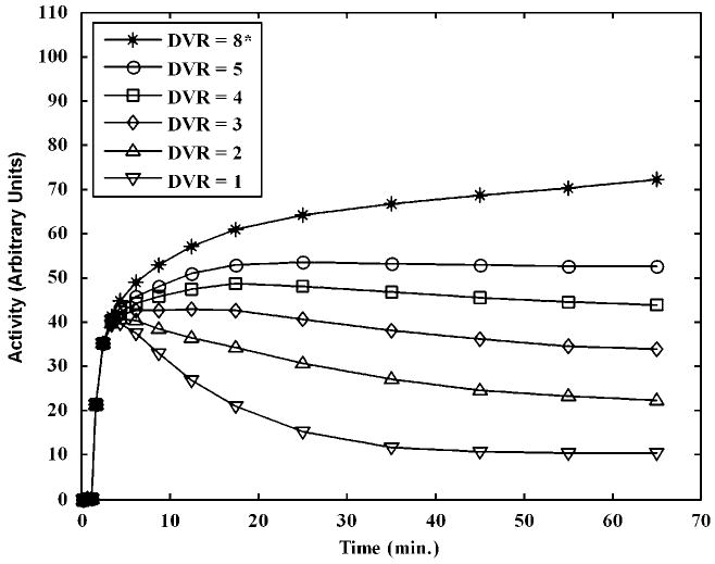
Noiseless time activity curves (TACs) for simulated test data. The test data comprised five hypothetical regions with receptor binding having true DVR values of 8, 5, 4, 3, and 2 and a reference region with no binding (DVR =1). The curve corresponding to DVR = 8* is an atypical curve that is not present in the training set. Realistic voxel-level noise was added to these noiseless curves to obtain 1,024 realizations for each DVR value.

It must be noted that as no blood samples are measured in reference region approaches, correction for blood volume component is not possible. Not correcting for blood volume component will introduce a systematic bias in the DVR estimates unrelated to the noise-induced bias (Logan et al, 1996). To check the magnitude of this systematic bias in the proposed and existing methods, separate simulations were also performed with blood volume component using the following model:

$$C(t)=V_{\text{B}}{C}_{\text{B}}(t)+(1-V_{\text{B}})C_{\text{T}}(t)$$ (10)

where C(t) is the total radioligand concentration measured in a voxel, V_B is the blood volume component (chosen to be 3.5%), and C_B(t) is the blood radioligand concentration.

Intervention Studies (Simulated Data)

Intervention studies were simulated with the same input function and rate parameters as for single-measurement studies (Table 1) with a naloxone intervention simulated 40 min after initiation of the scan. The simulated data consisted of 100 min, 19-frame scan (4 × 0.5 min, 3 × 1 min, 2 × 2.5 min, 2 × 5 min, and 8 × 10 min), which is the same protocol used for human intervention scans at our institution. The training set consisted of TACs with a linear decrease in k₃ to 40%, 50%, and 60% of the initial k₃ value over 10 min after the intervention to model the loss in binding potential after the naloxone intervention. The test set was simulated with a 50% decrease in k₃. The DVR values were estimated from Logan plots using ‘early’ data from 20 to 40 min for pre-intervention DVR (DVR_pre) and ‘late’ data from 60 min until the end of scan data for post-intervention DVR (DVR_post) as shown in Figure 2 (noiseless case). DVR_pre is estimated from 20 to 40 min, when the Logan plot has become linear. The perturbation at 40 min (denoted by the vertical gray line) increases receptor occupancy causing the Logan plot to bend (40 to 60 min) before becoming linear again at around 60 min. The 60 to 100 min period can be used to estimate DVR_post. For both DVR_pre and DVR_post estimations, the integral terms in the numerators of equation (5) are calculated from the beginning of the scan.

Figure 2.

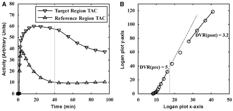
Dual-Logan approach for measurement of the in vivo distribution of a radiotracer before and after perturbation of the system in a single PET study. In the simulation study shown here (noiseless case), a ‘perturbation’ of the system is made 40 mins into the scan. The simulation was for a decrease in the binding potential of the target region by 50% (A). A Logan plot is used to estimate DVR both before and after the intervention (B). The gray lines indicate the point at which the ‘perturbation’ occurs.

Existing Bias-Removal Methods

DVR values for the above simulations were also estimated using existing bias-removal techniques. Thus, DVR values were estimated by the following six methods:

1. ordinary least squares (OLS) (Logan et al, 1996)

2. total least squares (TLS) (Varga and Szabo, 2002)

3. generalized linear least squares (GLLS) (Logan et al, 2001)

4. likelihood estimation graphical analysis (LEGA) (Ogden, 2001)

5. multilinear analysis-1 (MA1) (Ichise et al, 2002)

6. principal component analysis (PCA)

The TLS method (Varga and Szabo, 2002) takes into account errors in both dependent and independent variables of the Logan plot to estimate DVR. This can be classified as a method using an alternate cost function. The LEGA (Ogden, 2001) and MA1 (Ichise et al, 2002) approaches can be classified as methods rearranging the original Logan plot equation. In LEGA, a rearrangement of the operational Logan plot equation makes the error term additive. The problem is then solved by maximum likelihood approach. In MA1, equation (5) is rearranged to bring the noisy term on one side of the equation and DVR is estimated by taking the ratio of two regression coefficients. The GLLS method (Logan et al, 2001) can be classified as a temporal smoothing method. In this method, each noisy TAC is separated into two segments, which are individually fitted to one compartment model using GLLS (Feng et al, 1996). The smoothed segments are put together to get a smooth TAC, which is then used to obtain Logan DVR estimates. Implementation of GLLS requires choosing the frame where the TAC is to be segmented. For single-measurement simulations, the 11th frame (15 to 20 min) was found to be the optimal segmentation point for bias reduction and was used as segmentation point for human data as well. The proposed PCA approach can also be classified as a temporal smoothing method where a PCA-based lower dimension linear model is used to reduce the noise in the tissue curves.

For intervention studies, the intervention is applied at the 14th frame (40 to 50 min) and DVR is estimated from the segments before and after the 14th frame using Logan analysis. As mentioned before, the existing methods, although proposed for single-measurement studies, are also applicable to ‘dual-Logan’ intervention studies. Although this is true for GLLS as well, some practical difficulties exist. To apply the GLLS method exactly as proposed by Logan et al (2001) in the dual-Logan case, temporal segments of the TAC before and after intervention may have to be further cleaved into two parts each. This, although possible, is not practical because of a limited number of points in the TACs (11 pre-intervention and 6 post-intervention). Thus, we implemented GLLS without dividing the segments before and after intervention any further. It should be noted that to fairly compare this method with the other methods, the segments before and after intervention may need to be separated further (work not done).

Single-Measurement Studies (Human Data)

To apply the proposed approach in single-measurement human PET studies, 12 subjects were imaged with [¹¹C]CFN for 70 min and binned into 16 frames (4 × 0.5 min, 3 × 1 min, 2 × 2.5 min, 2 × 5 min, and 5 × 10 min). All scans were performed on a Siemens ECAT Exact HR+ scanner. Images were reconstructed after Fourier rebinning using 2D ordered subsets expectation maximization, 4 iterations, 16 subsets, and no postprocess smoothing, resulting in images with isotropic resolution of approximately 6 mm FWHM. Injected doses of [¹¹C]CFN were 555 to 666 MBq (15 to 18 mCi) at a specific activity of > 2,000Ci/mmol. Carfentanil was administered as partial bolus followed by continuous infusion. Subject motion across frames was corrected using Neurostat (University of Michigan; Minoshima et al, 1994, 1993). Volumes of interest, including the occipital cortex reference region, were obtained using a standardized volume-of-interest template after reorientation and nonlinear warping to the stereotactic Talairach atlas (Talairach and Tournoux, 1988) using Neurostat routines. DVR parametric images were obtained using the proposed and existing methods. The PCA training set consisted of TACs from all the individual voxels in the brain volume and was used to obtain the principal components for each subject. The system matrix was then constructed using the first ‘q’ principal components (‘q’ selected from simulations). All individual voxel TACs in the image volume were then fitted to the system matrix to obtain smooth TACs with reduced noise. DVR values were estimated by substituting these smoothed TAC values in place of the noisy TAC values in the denominators of equation (5). DVR estimates were also obtained by using the existing bias-removal methods and compared with the proposed PCA approach.

Intervention Studies (Human Data)

To apply the proposed approach in intervention studies, four human studies were performed using [¹¹C]CFN with a naloxone dose administered starting 40 min after CFN administration, to block tracer binding. Naloxone was administered as a 0.004 mg/kg bolus followed by 0.00004 mg per kg per min for the remainder of the study, a dosage designed to block approximately 50% of the specific binding sites. Four control subjects were also imaged where no intervention was given during the scan and thus no change in binding was expected between ‘early’ and ‘late’ DVR estimates. Data for these eight subjects were collected as in the single-measurement studies except that scans were acquired for 100 min and binned into 19 frames (4 × 0.5 min, 3 × 1 min, 2 × 2.5 min, 2 × 5 min, and 8 × 10 min). Except for the temporal range of data used, the procedure for estimating DVR using the proposed and existing methods in intervention studies is same as that for single-measurement studies as explained above.

Results

Single-Measurement Studies (Simulated Data)

The mean vector (η̄) and first three principal components (f̄₁, f̄₂, and f̄₃) obtained from the simulated CFN training data without blood volume component are shown in Figure 3. The first three components had eigenvalues of 1.24 × 10³, 278.75, and 7.91, respectively, whereas the second last and last components had eigenvalues of 6.36 × 10⁻³² and < 10⁻⁵⁰, respectively. This progression of eigenvalues (eigenvalue_i–1 ≫ eigenvalue_i) indicates that the first few components are the dominant vectors and capture most of the variance in the training set. The box plots in Figure 4 show the comparison of DVR estimates obtained using OLS with those estimated by increasing numbers of components for true DVR = 5 (PCAn⇒ G = [η̄f̄₁f̄₂ ⋯ f̄_n]). In the proposed PCA approach, we fit the noisy TACs as a linear combination of the mean vector in addition to the chosen principal components (16 possible components). In all, 17 PCA-based models are possible; the model with the smallest degrees of freedom is PCA0 with the mean vector alone G = [η̄]), and the one with the largest degrees of freedom is PCA16 with mean vector and all the 16 principal components (G = [η̄f̄₁ f̄₂ ⋯ F̄₁₆]). Too few components were insufficient to model the data and yielded biased estimates with high precision, as seen for PCA0, which used only the scaling of the mean vector. As the number of components was increased, the bias was reduced at the expense of precision (PCA1, PCA2, and PCA3). However, as the number of components exceeded three, the bias returned, as the added components began to fit noise in the data. Using all the 16 principal components (PCA16), as expected, gave back the original noisy data, and the box plot in this case is identical to the box plot for OLS. As we include the mean vector in all the PCA models, PCA15 (the mean vector and 15 components) can perfectly describe the 16-frame data. Thus, PCA15 and PCA16 give identical results.

Figure 3.

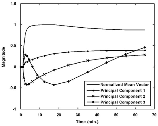
Mean vector and first three principal components for carfentanil-like tracer simulation studies. The mean vector is the mean of the entire training data whereas the three principal components are the dominant vectors obtained from PCA with the three largest eigenvalues.

Figure 4.

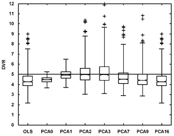
Box plot comparisons of DVR estimates obtained with an increasing number of principal components in single-measurement simulation studies (true DVR = 5). The individual boxes have lines at the lower, median, and upper quartile values. The whiskers extend from the ends of the box to the most extreme value within three times the interquartile range in each direction. DVR estimates beyond the whiskers are marked as outliers (denoted by ‘ + ’). PCAn ⇒ PCA fit with the first n principal components and the mean vector. When all 16 components are used (PCA16), the results are identical to the original OLS estimation.

The PCA1 (G = [η̄ f̄₁]) provided the best bias-variance trade-off for true DVR = 5. This implied that a linear combination of only two curve shapes could sufficiently approximate the simulated test data with DVR = 5 (q = 1). To check the validity of this finding for all the simulated TACs in the test set, we analyzed the residuals between the true noise-less TACs $\left({\overline{y}}_j^{\mathit{\text{true}}}\right)$ and the PCA1-fitted TACs ( ${\widehat{\overline{y}}}_j^{\mathit{\text{PCA}}1}$, 1≤ j ≤1,024). For the jth realization, the residual at the ith frame is given by ${\mathit{\text{residual}}}_j\left(T_i\right)={\overline{y}}_j^{\mathit{\text{true}}}\left(T_i\right)-{\widehat{\overline{y}}}_j^{\mathit{\text{PCA}}1}\left(T_i\right)$ (1≤ i ≤ p, where p = 16 is the number of frames in the study). These residuals were normalized by the true tissue curve values to obtain the percent-normalized residuals

$$=\left({\mathit{\text{residual}}}_j\left(T_i\right)/{\overline{y}}_j^{\text{true}}\left(T_i\right)\right)\times 100.$$

For a model to be valid, the mean of these percent-normalized residuals must lie close to zero (Carson, 1986). Figure 5 shows that for TACs with receptor binding that were part of the training set (DVR = 5, 4, 3, and 2), the mean of percent-normalized residuals was close to zero (between + 3% and −3%). For reference region TAC (DVR = 1, k₃ = 0) and for the atypical TAC not included in the training set (DVR = 8), the mean of the percent-normalized residuals was significantly different from zero, indicating that PCA1 was not a valid model for these curves. This makes intuitive sense as the reference region curve (shown in Figure 1, DVR = 1) has a more complicated shape compared with the curves with receptor binding because of rapid clearing of the tracer. The PCA3 (mean vector and three components) approach was found to be a valid model for the reference region. It should be pointed out that the actual reference region TAC used in the Logan plot calculations is not fitted using PCA but is the raw TAC. As the reference region is not derived from a single voxel, but is obtained from a volume of interest large enough to have minimal statistical noise, the raw reference region curve can be used for all DVR estimations without introduction of bias or loss of precision. Furthermore, the DVR estimates in regions of very low binding were found to be nearly unbiased even with nonzero residuals resulting for the PCA1 fit as seen in the last column of Table 2.

Figure 5.

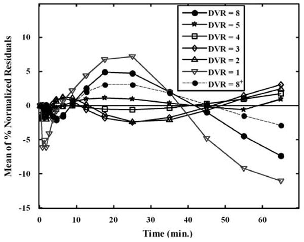
The mean of percent-normalized residuals between the PCA1-based curve approximations and the true tissue curves in single-measurement simulation studies. The plot indicates that PCA1 model is valid for TACs with receptor binding that were part of the training set (DVR = 5, 4, 3, and 2). For reference region curve (DVR = 1) and atypical curve not part of the training set (DVR = 8), however, the model is not valid, as the mean of percent-normalized residuals is significantly different from zero. Including curves similar to the atypical curve in the simulated training set (1% of the total curves) improves the fit (DVR = 8⁺).

Table 2.

Bias, given as percent of true value, and standard deviation in units of percent of true value (n = 1,024)

	DVR = 8	DVR = 8a	DVR = 5	DVR = 4	DVR = 3	DVR = 2	DVR = 1
OLS	77.7 (13.8)		87.1 (12.5)	90.1 (11.5)	92 (10.8)	94.9 (9.0)	97.2 (7.3)
TLS	93.5 (23.5)		95.6 (17.5)	94.8 (13.9)	95.4 (12.1)	96.2 (9.6)	97.4 (7.4)
GLLS	95.4 (26.2)		99.8 (20.0)	99.7 (15.3)	100.7 (13.5)	100.0 (10.3)	98.4 (8.1)
LEGA	100.0 (19.7)		105.5 (22.6)	102.5 (16.9)	102.2 (13.9)	102.2 (11.2)	101.4 (8.5)
MA1	107.4 (34.6)		106.9 (24.9)	103.4 (17.1)	102.9 (14.0)	102.9 (11.2)	103.1 (8.8)
PCA1	87.7 (7.3)	91.1 (9.7)	100.1 (8.1)	101.0 (8.1)	101.3 (8.9)	102.0 (8.3)	97.2 (7.2)
PCA2	98.0 (19.0)	99.2 (16.9)	102.6 (16.3)	102.6 (14.9)	102.8 (12.2)	101.9 (10.2)	98.1 (7.6)

Abbreviations: DVR, distribution volume ratio; GLLS, generalized linear least squares; LEGA, likelihood estimation graphical analysis; MA1, multilinear analysis-1; OLS, ordinary least squares; PCA, principal component analysis; TLS, total least squares.

A value of 100 represents ‘no bias’.

^aPCA training set including curve shapes similar to the atypical curve (1% of total curves).

Invalidity of the PCA1 model for the atypical curve is also expected, as the success of the PCA-based approach depends on the diversity of the training set, and if a curve shape is significantly different from any in the training set, the PCA1 model may not be adequate. However, in human studies, the training set consists of all the TACs in the PET image volume. Thus, a region with unusual kinetics, if any, will contribute curves to the training set. If we include curves similar to the atypical curve in the simulated training set (1% of the total curves), the fit improves as seen in Figure 5 (DVR = 8⁺).

The standard deviations of the percent-normalized residuals for PCA1-based TACs calculated above were approximately 50% of that for original noisy tissue curves. Thus, from this result and Figure 5, we could conclude that PCA1 model was valid for the curves with receptor binding that were part of the training set and provided TACs with reduced noise.

More detailed results have been presented for the curve simulated with DVR = 5. The histograms in Figure 6 show the distribution of the DVR values estimated by each of the existing methods versus PCA1. A Gaussian kernel with unbounded support was used to smooth the histograms. These plots were useful for visualizing asymmetries and tails in the distribution of the estimated DVR values. The vertical line denotes the ‘true’ DVR value. The modes of the histograms of all the existing methods either lie below the true DVR value, show heavy tails, or both. The PCA approach has its mode at the true value but has a heavier tail than PCA1. The PCA approach was seen to be superior to all the existing methods. Figure 7 depicts the trade-off between precision and bias in the DVR estimates of the different approaches, again for DVR = 5. An ideal estimator has no bias and minimal variance, and would lie near the origin. The OLS method (superimposed with PCA16) is on the far right, denoting the bias present because of noise. The TLS method removes only a portion of the bias. The GLLS, LEGA, MA1, PCA2, and PCA3 methods reduce the bias but also have poorer precision. The PCA1 method shows the best performance and is closest to the origin than any other method. Figure 8 shows box plots for DVR estimates from all methods (DVR = 5). The median and range of DVR estimates using OLS are below the true value, as expected. The bias in the median is reduced only slightly using TLS with a decrease in precision. The GLLS, LEGA, MA1, and PCA2 methods reduce the bias almost entirely but have high variance. Principal component analysis 1 eliminates bias almost completely and yields the best precision estimates compared with any of the methods.

Figure 6.

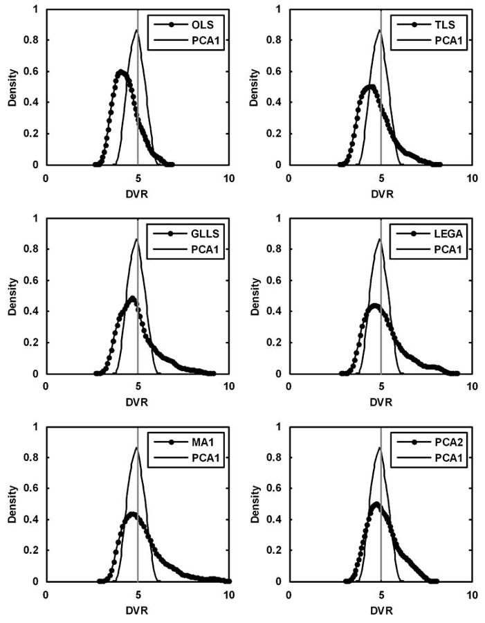
Comparison of distribution of the DVR values estimated by each of the existing methods versus PCA1 in single-measurement simulation studies for true DVR = 5 (discarding the top and bottom 2.5 percentiles). The TLS, GLLS, and LEGA methods have modes lower than the true value but higher than that for OLS. Multilinear analysis-1 has a heavier tail because of overestimations. The PCA1 method proves to be the best estimator with a narrow, unbiased distribution as compared with all the other methods. The distribution of DVR estimates with PCA2 has its mode at the true value but has a heavier tail than PCA1.

Figure 7.

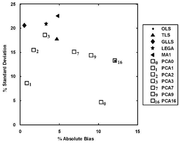
Trade-off between bias and precision for the existing and proposed bias-removal methods in single-measurement simulation studies (discarding the top and bottom 2.5 percentiles). The plot shows percent absolute bias versus percent standard deviation for true DVR = 5. The original OLS method shows high bias, which is removed at the expense of some increase in estimation variability by the existing bias-removal methods. If the proposed method was underparameterized (PCA0) or overparameterized (PCA7, PCA9, and PCA16), bias returned. The PCA1 approach yielded the best compromise between bias and precision.

Figure 8.

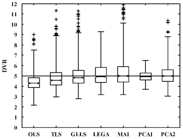
Box plot comparisons of the DVR estimates obtained using the existing bias-removal methods and the proposed bias-removal method for single-measurement simulation studies (true DVR = 5). The TLS method reduces only part of the bias, whereas GLLS, LEGA, and PCA2 (with a wide interquartile distance) and MA1 (with large number of outliers) reduce most of the bias but at the expense of precision. The PCA1 approach reduces bias along with an improvement in estimation precision.

Table 2 summarizes the means and standard deviations of the estimated DVR values in units of percentage of true value for all the simulated test curves. Although the trends for DVR<5 (last four columns) are similar to those seen in Figure 8 (DVR = 5), bias for OLS is lower for curves with lower DVR values, as expected (Slifstein and Laruelle, 2000). The first two columns show the statistics for the atypical TAC with bias in the PCA1 estimate of DVR when the atypical curve is not part of the training set (DVR = 8, column 1), and reduction in bias when atypical curve shapes are included in the training set (DVR = 8^a, column 2). Inclusion of curve shapes similar to the atypical curve in the training set (1% of total curves) improves the fit but does not remove the bias completely for PCA1. The representation of atypical curve shapes in the training set was required to be at least 5% for the bias to be removed completely for PCA1. Thus, very small regions with unusually shaped TACs, if identified before Logan analysis, could be fitted with PCA2, where bias is removed almost completely but at the expense of precision.

Figure 9 shows the box plot for DVR estimates from all methods for curves simulated with but not corrected for the blood volume component (DVR = 5). The box plots have similar bias–variance trends as in Figure 8, apart from the consistent bias seen in Figure 9 for all methods because of uncorrected blood volume component. This bias is minimal (<5%) compared with the noise-induced bias in OLS (>10%) for DVR = 5 and is even smaller for lower DVR values.

Figure 9.

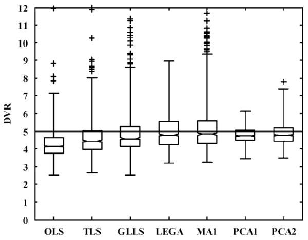
Box plot comparisons of the DVR estimates obtained using the existing and proposed bias-removal methods for single-measurement studies simulated with but without correcting for blood volume component (true DVR = 5). The trends are similar to those seen in Figure 8 along with a consistent but minimal bias (<5%) as compared with the noise-induced bias in OLS (>10%).

Trends similar to those seen in Figures 4–9 were seen for simulations of different levels of noise (results not shown).

Intervention Studies (Simulated Data)

Analyses similar to those shown in Figures 4–9 were performed for intervention studies to determine the appropriate number of principal components for fitting the noisy data. Figure 10 shows percent absolute bias versus percent standard deviation in the DVR estimates for both pre-intervention (‘true’ DVR_pre = 5) and post-intervention (‘true’ DVR_post= 3) data. As the bias in the estimated DVR values is higher for larger DVR values, in general the bias is higher in DVR_pre than DVR_post. It can be seen that PCA1(pre) and PCA3(post) provide the best bias– variance trade-off (by virtue of their proximity to the origin) compared with all the other methods. In fact, DVR estimates using all PCA-based approaches tested (PCA1, PCA2, and PCA3) cluster close to the origin and reduce bias while maintaining good precision. All the existing bias-removal methods reduce bias at the expense of precision.

Figure 10.

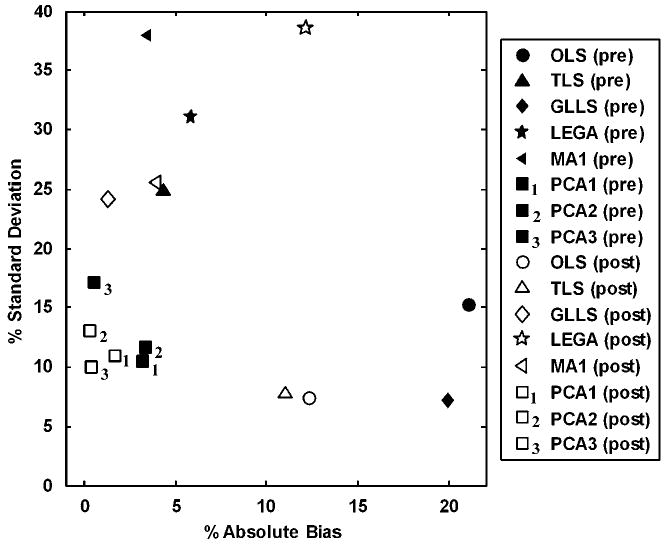
Comparison of DVR estimation using existing and proposed bias-removal methods for simulated intervention studies (discarding the top and bottom 2.5 percentiles). The figure shows the percent standard deviation versus percent absolute bias in DVR_pre and DVR_post for the simulation studies, where the binding density was decreased by 50% postintervention. ‘True’ DVR_pre and DVR_post were 5 and 3, respectively. The OLS method showed the maximum bias similar to single-measurement studies. All the PCA-based methods (PCA1, PCA2, and PCA3) cluster close to the origin and reduce bias while maintaining good precision. The existing bias-removal techniques reduce the bias at the expense of an increase in variance.

Single-Measurement Studies (Human Data)

For the 12 human scans in the single-measurement case, eight regions of interest were placed on the estimated DVR images of each subject obtained from all the methods. The means of DVR values and means of the standard deviations within these regions from 12 subjects are reported in Table 3. The top 50 percentile pixels in these regions of interest were used to obtain the statistics. The performance of the methods in the human data was seen to match closely with the performance in simulation studies. The TLS estimates are higher but quite close to that of OLS for all regions. The estimates of GLLS, LEGA, PCA1, PCA2, and PCA3 are higher than OLS as seen in single-measurement simulation studies indicating reduction in bias. Mean values for MA1 are higher than the other methods because of the presence of outliers. The means of the standard deviations (across-subject means of the within-region standard deviations) also follow the same trend as seen in simulations with PCA1 having the lowest and MA1 having the highest variance compared with the other methods. It is important to note that in general the PCA method yields the smallest standard deviations, which is the strength of the approach.

Table 3.

Mean DVR (mean standard deviation) in subjects imaged with the single-measurement protocol (n = 12)

	Thalamus	Dorsal caudate	Ventral caudate	Amygdala	Anterior cingulate	Cortex	Cerebrum	Occipital cortex
OLS	2.68 (0.23)	2.51 (0.48)	2.82 (0.42)	2.56 (0.53)	1.79 (0.54)	1.52 (0.22)	1.68 (0.18)	1.10 (0.22)
TLS	2.74 (0.26)	2.55 (0.63)	2.92 (0.47)	2.70 (0.69)	1.81 (0.71)	1.53 (0.25)	1.69 (0.20)	1.10 (0.23)
GLLS	2.83 (0.24)	2.62 (0.43)	3.05 (0.39)	2.85 (0.45)	1.85 (0.39)	1.56 (0.22)	1.73 (0.19)	1.12 (0.22)
LEGA	2.90 (0.37)	2.68 (0.68)	3.18 (0.59)	2.98 (0.85)	1.89 (0.83)	1.61 (0.34)	1.78 (0.34)	1.17 (0.31)
MA1	3.13 (1.33)	3.44 (2.95)	3.25 (2.27)	3.15 (3.54)	1.92 (3.69)	1.67 (1.43)	1.78 (1.28)	1.24 (1.10)
PCA0	2.64 (0.17)	2.49 (0.21)	2.71 (0.17)	2.39 (0.24)	1.86 (0.14)	1.54 (0.17)	1.78 (0.11)	1.07 (0.16)
PCA1	3.03 (0.22)	2.77 (0.35)	3.30 (0.31)	3.16 (0.38)	1.89 (0.31)	1.59 (0.20)	1.77 (0.16)	1.11 (0.23)
PCA2	2.87 (0.24)	2.64 (0.43)	3.06 (0.38)	2.83 (0.45)	1.88 (0.44)	1.58 (0.22)	1.75 (0.19)	1.12 (0.23)
PCA3	2.87 (0.26)	2.63 (0.51)	3.06 (0.45)	2.83 (0.59)	1.88 (0.55)	1.58 (0.24)	1.75 (0.21)	1.12 (0.23)

Abbreviations: DVR, distribution volume ratio; GLLS, generalized linear least squares; LEGA, likelihood estimation graphical analysis; MA1, multilinear analysis-1; OLS, ordinary least squares; PCA, principal component analysis; TLS, total least squares.

Mean standard deviation is the across-subject mean of the within-region standard deviation.

Intervention Studies (Human Data)

Figure 11 shows DVR images obtained from the data obtained before and after 40 min of scanning in one of the control subjects where no intervention was given; hence, DVR_pre and DVR_post images should be identical. The OLS, TLS, and GLLS methods show a decrease in global DVR, although no receptor blocking in present. The LEGA and MA1 methods give noisy DVR images, especially for the ‘late’ measure, and hence should not be used to create parametric images in intervention studies. The PCA1 images show little to no change between ‘pre’ and ‘post’ images and do not show any bad fits. The PCA2 and PCA3 images show higher variance but little to no change between early and late DVR images. To quantify these effects, scatter plots of pre and post binding potential estimates for voxels with receptor binding (BP_ND > 1) were made for all the subjects, and the mean values of correlation coefficient, slope, and intercept are reported in Table 4 (n = 4 for both groups). As errors exist in both abscissa and ordinate, the regression slopes and intercepts were estimated using TLS optimization.

Figure 11.

DVR images from a representative control subject estimated from data obtained before and after 40 mins with no intervention. The OLS, TLS, and GLLS show a decrease in global DVR values despite there being no intervention. Likelihood estimation graphical analysis and MA1 give very noisy results. Principal component analysis 1 yields images with high precision for both ‘pre-’ and ‘post’ estimation periods with no noticeable difference in binding magnitudes between the two estimations.

Table 4.

Mean correlation coefficient, mean slope, and mean intercept of the scatter plots of the early and late BP_ND estimates in control subjects with no intervention (n = 4) and with naloxone intervention (n = 4)

	No intervention (control)			With naloxone intervention
	Correlation coefficient	Slope	Intercept	Correlation coefficient	Slope	Intercept
OLS	0.83 (0.02)	0.82 (0.06)	−0.01 (0.02)	0.75 (0.04)	0.44 (0.03)	0.05 (0.03)
TLS	0.80 (0.02)	0.81 (0.08)	−0.01 (0.03)	0.73 (0.04)	0.41 (0.03)	0.06 (0.03)
GLLS	0.84 (0.01)	0.99 (0.08)	−0.12 (0.03)	0.84 (0.03)	0.66 (0.02)	−0.08 (0.01)
LEGA	0.57 (0.07)	1.41 (0.25)	−0.33 (0.17)	0.44 (0.05)	1.01 (0.54)	−0.38 (0.43)
MA1	0.28 (0.04)	2.18 (0.74)	−0.96 (0.59)	0.13 (0.05)	0.30 (0.24)	0.22 (0.25)
PCA1	0.99 (0.00)	0.96 (0.04)	−0.02 (0.01)	0.93 (0.03)	0.54 (0.04)	−0.15 (0.04)
PCA2	0.91 (0.06)	0.96 (0.04)	−0.04 (0.02)	0.84 (0.09)	0.51 (0.03)	0.08 (0.01)
PCA3	0.89 (0.04)	0.93 (0.06)	−0.03 (0.02)	0.80 (0.09)	0.43 (0.04)	−0.00 (0.04)

Abbreviations: BP_ND, nondisplaceable binding potential; GLLS, generalized linear least squares; LEGA, likelihood estimation graphical analysis; MA1, multilinear analysis-1; OLS, ordinary least squares; PCA, principal component analysis; TLS, total least squares.

The values in parentheses are standard deviations from the reported statistics. A total least squares optimization was used to calculate the regression slope and intercept, as errors exist in both abscissa and ordinate measures.

In the case of the controls, the ideal estimator will have correlation coefficient = 1 and slope = 1, with intercept at the origin indicating no variance and no change in occupancy. The PCA1 method behaves closest to the ideal estimator for the control case. The other methods show lower correlations and slopes less than 1, indicating higher variance and an apparent change in occupancy because of higher bias in ‘late’ than in ‘early’ DVR estimates. Figure 12 shows DVR images before and after intervention in one of the subjects who received naloxone. Noise properties of DVR images are similar to those in the no intervention case. The OLS, TLS, and GLLS methods show the expected decrease but are noisier. Similar to the results in the control study, LEGA and MA1 images are much noisier and would have limited utility for intervention studies. The PCA1 images have the lowest variance and show the expected decrease in DVR values; PCA2 and PCA3 again have higher variance, but show the expected effects of naloxone on DVR estimates. The results for scatter plots in the naloxone intervention cases are summarized in Table 4 (right columns). The PCA-based methods have higher correlations than the other methods and the mean slope for PCA1 = 0.54 corresponds well with the expected ∼50% occupancy of receptor sites at the chosen naloxone dose.

Figure 12.

DVR images from a representative subject from scan data before and after injecting naloxone (40 mins after the beginning of radiotracer administration). The OLS, TLS, and GLLS show the expected decrease in global DVR values but lack precision in voxelwise estimates. As in the control study, LEGA and MA1 yield images that are very noisy. The PCA1 method produces high-precision images for both early and late data and shows the expected decreases in binding values because of naloxone.

The performance of each method varied little from subject to subject, as seen by the small across-subject standard deviation values for the mean statistics as reported in Table 4. The performance of all the methods depends primarily on the noise level in the TACs (higher bias and variance with higher noise). As all the subjects were imaged with the same PET scanner, the noise level in all scans was similar and so was the performance of each method from subject to subject.

Discussion

The negative bias in the DVR estimates from Logan plots is because of the noise in the PET TACs that propagates as correlated errors in dependent and independent variables of the Logan plot equation. Although several methods for reducing this bias have been proposed, these methods either remove only a portion of the bias, or reduce bias at the expense of precision. Parameter estimation by TLS removes only a portion of the bias. The GLLS, LEGA, and MA1 methods are quite effective in removing bias, but show poorer precision, especially for intervention studies where two DVR estimations are required. In the proposed approach, fitting the dynamic PET data to a low-dimension PCA-based linear model maintains the appropriate kinetic shape of the TACs while removing noise and hence the source of the correlated errors in the Logan plot equation. This provides DVR estimates with minimal bias and reduced variance. In single-measurement simulation studies, the linear combination of just two curve shapes (the mean vector and first principal component) was successful in modeling the simulated test data curves sampled from the training set and reduced bias and variance associated with their DVR estimates. If a test data curve was not part of the training set, PCA1 was insufficient to model it, leading to bias in DVR estimates as seen for the atypical curve (DVR = 8). In human studies, however, TACs from all the voxels in the image volume are used as training data to obtain the PCA-based linear model. A region of unusual kinetics, if present, will contribute to the total TACs in the training data. Thus, a region of unusual kinetics contributing 1% of the total TACs to the training data was simulated. By including curve shapes similar to the one with DVR = 8 in the training set (1% of total curves), the bias in DVR estimates was reduced but not completely removed. Small regions with atypical TACs, if identified before DVR estimation, could be fitted with PCA2, where bias will be removed at the expense of precision.

Adding another component to the PCA1 model (PCA2) also removed bias, but increased the variance of the DVR estimates. Although the increase in variance between PCA1 and PCA2 is expected because of an increase in degrees of freedom, the magnitude of this increase will vary from tracer to tracer and will depend on the particular curve shapes under consideration, and thus needs to be evaluated for each radiotracer application.

Another source of bias, unrelated to the noise-induced bias, exists for reference region approaches because of lack of accounting for the blood-borne component of the PET signal. This was observed to cause a small but consistent bias in all the methods, but was minor compared to the noise-induced bias in OLS.

It should be pointed out that in both the simulation studies and the human scans, we used a partial bolus followed by continuous infusion for administration of the radiotracer. This may reduce the kinetic complexity of the TACs compared to bolus injection studies, and hence limit the number of principal components required to describe the shape of the TACs. When applying the PCA approach to other PET ligands or radiotracer administration protocols, the optimal number of components for describing the TAC shapes needs to be reevaluated. However, in our experience, the mean vector plus at most two principal components seem sufficient for modeling standard single-measurement PET studies for most radiotracers, whereas the mean vector plus at most three components are sufficient for interventional PET studies that may have more complex kinetic behavior.

Obtaining the components from training data has a closed-form solution and hence is not computationally expensive. While the simulation studies are a necessary step in the validation of any newly proposed approach, the final evaluation must involve real data. Results presented in Tables 3 and 4 and Figures 11 and 12 clearly show the utility of the PCA approach in human data. In particular, it should be emphasized that for intervention studies, the PCA approach is the only approach that produced voxel-by-voxel parametric images with acceptable noise levels and with little observable bias. Figure 11 shows that for the no-intervention case, only PCA1 yielded ‘early’ and ‘late’ DVR values that were of the same magnitude and of the same statistical quality. A similar advantage of PCA1 compared with the other methods for the intervention case is seen in Figure 12, with the expected decrease in DVR because of naloxone. Scatter plots of pre- versus post-intervention binding potential estimates show that PCA-based methods yield the highest correlation and have closer to the expected slopes compared with the other methods (Table 4). These results show both the sensitivity and specificity of the PCA-based approach. The PCA1 approach produced unchanged ‘early’ and ‘late’ measures when no intervention was given, and also showed the ability to detect intervention-induced changes when present. The PCA1 method, however, may not have the necessary degrees of freedom to model very large displacements. The PCA2 or PCA3 methods will capture these large displacements, but at the expense of higher variance.

The proposed PCA method is simple to implement and computationally fast. For relatively slowly equilibrating tracers like [¹¹C]CFN, PCA1 produced DVR images that had less bias, lower variance, or both, compared with existing bias-removal methods. Advantages of the PCA approach were seen not only for standard single-measurement PET studies, but were especially impressive when applied to dual-measurement intervention studies where pre- and post-challenge DVR estimates are required.

References

- Barber DC. The use of principal components in the quantitative analysis of gamma camera dynamic studies. Phys Med Biol. 1980;25:283–92. doi: 10.1088/0031-9155/25/2/008. [DOI] [PubMed] [Google Scholar]
- Carson RE. Parameter estimation in positron emission tomography. In: Phelps M, Mazziotta J, Schelbert H, editors. Positron emission tomography and autoradiography: principles and applications for brain and heart. New York: Raven Press; 1986. pp. 347–90. [Google Scholar]
- Endres CJ, Bencherif B, Hilton J, Madar I, Frost JJ. Quantification of brain mu-opioid receptors with [11C]carfentanil: reference-tissue methods. Nucl Med Biol. 2003;30:177–86. doi: 10.1016/s0969-8051(02)00411-0. [DOI] [PubMed] [Google Scholar]
- Faraway J. Linear models with R. Chapman & Hall/CRC; Boca Raton: 2004. Principal components; pp. 131–7. [Google Scholar]
- Feng D, Huang SC, Wang Z, Ho D. An unbiased parametric imaging algorithm for nonuniformly sampled biomedical system parameter estimation. IEEE Trans Med Imag. 1996;15:512–8. doi: 10.1109/42.511754. [DOI] [PubMed] [Google Scholar]
- Ichise M, Toyama H, Innis RB, Carson RE. Strategies to improve neuroreceptor parameter estimation by linear regression analysis. J Cereb Blood Flow Metab. 2002;22:1271–81. doi: 10.1097/01.WCB.0000038000.34930.4E. [DOI] [PubMed] [Google Scholar]
- Kadrmas DJ, Rust TC. Feasibility of rapid multi-tracer PET tumor imaging. IEEE Trans Nucl Imag. 2005;52:1341–7. [Google Scholar]
- Kimura Y, Senda M, Alpert NM. Fast formation of statistically reliable FDG parametric images based on clustering and principal components. Phys Med Biol. 2002;47:455–68. doi: 10.1088/0031-9155/47/3/307. [DOI] [PubMed] [Google Scholar]
- Koeppe RA. Dual logan plot analysis for PET studies with pharmacological challenge. NeuroImage. 2002;16:S54. [Google Scholar]
- Logan J, Fowler JS, Volkow ND, Ding YS, Wang GJ, Alexoff DL. A strategy for removing the bias in the graphical analysis method. J Cereb Blood Flow Metab. 2001;21:307–20. doi: 10.1097/00004647-200103000-00014. [DOI] [PubMed] [Google Scholar]
- Logan J, Fowler JS, Volkow ND, Wang GJ, Ding YS, Alexoff DL. Distribution volume ratios without blood sampling from graphical analysis of PET data. J Cereb Blood Flow Metab. 1996;16:834–40. doi: 10.1097/00004647-199609000-00008. [DOI] [PubMed] [Google Scholar]
- Minoshima S, Koeppe RA, Frey KA, Kuhl DE. Anatomical standardization: linear scaling and nonlinear warping of functional brain images. J Nucl Med. 1994;35:1528–37. [PubMed] [Google Scholar]
- Minoshima S, Koeppe RA, Mintun MA, Berger KL, Taylor SS, Frey KA, Kuhl DE. Automated detection of the intercommissural (AC-PC) line for stereotactic localization of functional brain images. J Nucl Med. 1993;34:322–9. [PubMed] [Google Scholar]
- Ogden RT. Estimation of kinetic parameters in graphical analysis of PET imaging data. Stat Med. 2001;22:3557–68. doi: 10.1002/sim.1562. [DOI] [PubMed] [Google Scholar]
- Pedersen F, Bergström M, Bengtsson E, Långström B. Principal component analysis of dynamic positron emission tomography images. Eur J Nucl Med. 1994;21:1285–92. doi: 10.1007/BF02426691. [DOI] [PubMed] [Google Scholar]
- Razifar P, Axelsson J, Schneider H, Långström B, Bengtsson E, Bergströmc M. A new application of pre-normalized principal component analysis for improvement of image quality and clinical diagnosis in human brain PET studies—clinical brain studies using [11C]- GR205171, [11C]-l-deuterium-deprenyl, [11C]-5-hydroxy-l-tryptophan, [11C]-l-dopa and Pittsburgh Compound-B. NeuroImage. 2006;33:588–98. doi: 10.1016/j.neuroimage.2006.05.060. [DOI] [PubMed] [Google Scholar]
- Sitek A, Di Bella EVR, Gullberg GT. Factor analysis of dynamic structures in dynamic spect imaging using maximum entropy. Trans Nucl Sci. 1999;46:2227–32. [Google Scholar]
- Slifstein M, Laruelle M. Effects of statistical noise on graphic analysis of PET neuroreceptor studies. J Nucl Med. 2000;41:2083–8. [PubMed] [Google Scholar]
- Talairach J, Tournoux P. Co-planar stereotaxic atlas of the human brain: 3-dimensional proportional system—an approach to cerebral imaging. New York, NY: Thieme Medical Publishers; 1988. [Google Scholar]
- Thireou T, Strauss LG, Dimitrakopoulou-Strauss A, Kontaxakis G, Pavlopoulos S, Santos A. Performance evaluation of principal component analysis in dynamic FDG-PET studies of recurrent colorectal cancer. Comput Med Imaging Graph. 2003;27:43–51. doi: 10.1016/s0895-6111(02)00050-2. [DOI] [PubMed] [Google Scholar]
- Varga JZ, Szabo Z. Modified regression model for the Logan plot. J Cereb Blood Flow Metab. 2002;22:240–4. doi: 10.1097/00004647-200202000-00012. [DOI] [PMC free article] [PubMed] [Google Scholar]