

Abstract
We developed a new method to estimate the spatial extent of summation, the cortical spread, of the local field potential (LFP) throughout all layers of macaque primary visual cortex V1 by taking advantage of the V1 retinotopic map. We mapped multi-unit activity and LFP visual responses with sparse-noise at several cortical sites simultaneously. The cortical magnification factor near the recording sites was precisely estimated by track reconstruction. The new method combined experimental measurements together with a model of signal summation to obtain the cortical spread of the LFP. This new method could be extended to cortical areas that have topographic maps such as S1 or A1, and to cortical areas without functional columnar maps, such as rodent visual cortex. In macaque V1, the LFP was the sum of signals from a very local region, the radius of which was on average 250 μm. The LFP's cortical spread varied across cortical layers, reaching a minimum value of 120 μm in layer 4B. An important functional consequence of the small cortical spread of the LFP is that the visual field maps of LFP and MUA recorded at a single electrode site were very similar. The similar spatial scale of the visual responses, the restricted cortical spread, and their laminar variation led to new insights about the sources and possible applications of the LFP.
Introduction
The local field potential (LFP) is comprised of the slow fluctuations (<100 Hz) of the voltage recorded by extra-cellular microelectrodes. The LFP has been studied in many different brain structures, such as V1, V4, MT, and IT, as well as olfactory, auditory, motor, frontal and parietal cortex and the hippocampus (Mitzdorf, 1987; Eckhorn et al., 1988; Victor et al., 1994; Kruse and Eckhorn, 1996; Fries et al., 2001; Logothetis et al., 2001; Rols et al., 2001; Brosch et al., 2002; Pesaran et al., 2002; Neville and Haberly, 2003; Gail et al., 2004; Henrie and Shapley, 2005; Rickert et al., 2005; Scherberger et al., 2005; Kreiman et al., 2006; Liu and Newsome, 2006; Womelsdorf et al., 2006; Pesaran et al., 2008; Sirota et al., 2008; Katzner et al., 2009). The LFP is of interest because: (1) the LFP is thought to sum the activity from many neurons (Mitzdorf, 1987; Buzsáki, 2004) revealing neuronal activity at the population level; (2) population activity measured by the LFP may be related to the BOLD signal in fMRI (Logothetis et al., 2001; Goense and Logothetis, 2008); (3) the LFP has become a candidate signal for neural prostheses because it is easier to record and more tolerant to recording position compared with spike activity (Andersen et al., 2004; Scherberger et al., 2005; Pesaran et al., 2006).
An important outstanding question is, what is the cortical spread of the LFP, or how far can the LFP propagate in cortical tissue? Although this question has been addressed many times (Mitzdorf, 1987; Victor et al., 1994; Kruse and Eckhorn, 1996; Gail et al., 2003; Kreiman et al., 2006; Liu and Newsome, 2006; Logothetis et al., 2007; Berens et al., 2008; Katzner et al., 2009), the conclusions from different studies are very different. Indeed, two recent studies of the LFP in V1 cortex (Berens et al., 2008; Katzner et al., 2009) use similar approaches yet reach very different conclusions about the LFP's spatial extent. Uncertainty about the cortical spread of the LFP makes it difficult to interpret or to use LFP measurements in applications like neural prostheses (Andersen et al., 2004; Scherberger et al., 2005; Pesaran et al., 2006).
In this study, we developed a new method to estimate the cortical spread of the LFP. This method could be applied to any cortical area with a topographic map, and unlike other methods (Liu and Newsome, 2006; Katzner et al., 2009) it does not require that the cortical area under study has a functional columnar map. Thus our approach could be used to study mouse visual cortex for example. The results of our new method applied to macaque V1 were that the LFP was the sum of cortical signals over a circular region ∼250 μm in radius, and also that there was clear laminar variation in the cortical spread of the LFP. Also, as a consequence of the small cortical spread of LFP signals, the LFP and multi-unit activity (MUA) recorded simultaneously had similar visual field maps. Therefore, the LFP is a good index of local circuit activity.
Materials and Methods
Surgery and preparation.
Acute experiments were performed on adult Old World monkeys (Macaca fascicularis). All surgical and experimental procedures were performed in accordance with the guidelines of the U.S. Department of Agriculture and were approved by the University Animal Welfare Committee of New York University. Animals were sedated with midazolam (0.3 mg/kg, i.m.) and anesthetized initially with ketamine (30 mg/kg, i.m.) and then with isofluorane (1.5–3.5% in air) after being intubated. After intravenous catheters were placed in both hindlimbs, the animal was placed in a stereotaxic frame and maintained on opioid anesthetic (sufentanil citrate, 6–12 μg · kg−1 · h−1, i.v.) during further surgery. A craniotomy (∼5 × 7 mm) was made in one hemisphere posterior to the lunate sulcus (∼15 mm anterior to the occipital ridge, ∼10 mm lateral from the midline). A small opening in the dura (∼3 × 5 mm) was made to provide access for multiple electrodes. After surgery, anesthesia was maintained with a continuous infusion of sufentanil citrate (6–12 μg · kg−1 · h−1, i.v.), and the animal was paralyzed with vecuronium bromide (0.1 mg · kg−1 · h−1, i.v.) and hydration was maintained by infusing fluid at a rate of ∼6 ml · kg−1 · h−1 (the infusion rate was adjusted hourly to keep the urine-specific gravity within the normal range (∼1.010 g/ml)). Vital signs, including heart rate, electroencephalogram, blood pressure, and oxygen level in blood were closely monitored throughout the experiment. Expired carbon dioxide partial pressure was maintained close to 32–38 mmHg and rectal temperature was kept at a constant 37°C using a feedback-controlled heating pad. A broad-spectrum antibiotic (Bicillin, 50,000 iu/kg, i.m.) and anti-inflammatory steroid (dexamethasone, 0.5 mg/kg, i.m.) were given on the first day and every 24 h during the experiment. The eyes were treated with 1% atropine sulfate solution to dilate the pupils and with a topical antibiotic (gentamicin sulfate, 3%) before being covered with gas-permeable contact lenses. Foveae were mapped onto a tangent screen using a reversing ophthalmoscope. The visual receptive fields of isolated neurons were later mapped on the same tangent screen, keeping reference to the foveae. Proper refraction was achieved by placing corrective lenses in front of the eyes on custom-designed lens holders. The eyes were stabilized with ophthalmic rings to minimize drift of visual field position.
Electrophysiological recordings and data acquisition.
A matrix of seven independently moveable electrodes (Thomas Recording) was used to record simultaneously from multiple cortical cells and sites in V1. The seven electrodes were arranged in a straight line with each electrode separated from its neighbor by ∼300 μm. Each electrode consisted of a platinum/tungsten core (25 μm in diameter and 1 μm at the tip) covered with an outer quartz-glass shank (80 μm in diameter), and had an impedance value of 1–4 MΩ. The multi-electrode matrix was precisely positioned before recordings so the tip of the matrix was ∼3 mm above the cortical surface. To keep all seven electrodes at approximately similar cortical depth, we independently moved each electrode from the surface of V1 until we got from each electrode a detectable high-frequency response that was driven by the visual stimulus. The high-frequency response (hash) represents multi-unit spike activity, and usually finding the first hash provided a very good estimation of the upper part of layer 2/3, and helped us to align all seven electrodes at a similar cortical depth (for an example, see Fig. 5A). Once all electrodes were placed in the superficial layer of V1, we built a chamber with bone wax to surround the multielectrode matrix and filled the chamber with a large amount of agar to seal the craniotomy entirely. We found this procedure largely enhanced the stability of recordings throughout the experiment. Then we conducted our experiments advancing the electrode matrix at ∼100 μm intervals in the cortex. This setup allowed simultaneous recordings of multiple neurons within the same cortical layer, all at nearby visual eccentricities. Electrical signals from the seven electrodes were amplified, digitized, and filtered (0.3–10 kHz) with a preamplifier (Tucker-Davis Technologies, model number: RA16SD) configured for multi-channel recording. The Tucker-Davis system was interfaced to a computer (Dell) running a multi-channel version of the OPEQ program (designed by Dr. J. A. Henrie, New York University, New York, NY) to acquire both spike and local field potential data. Visual stimuli were generated also with the custom OPEQ program running in a Linux computer (Dell) with a graphics card with Open GL optimization. Data collection was synchronized with the screen refresh to a precision of <0.01 ms. Stimuli were displayed on a 20-in monitor (IIyama HM 204DTA flat Color Graphic Display; pixels: 1024 × 768; frame rate: 100 Hz; mean luminance: 59.1 cd/m2) with a screen viewing distance of ∼114 cm. The basic attributes of each cell were estimated using small drifting sinusoidal gratings surrounded by a gray background (both the gratings and the gray background had a mean luminance of 59.1 cd/m2).
Figure 5.

Model schematic: visual spread and cortical spread of the LFP and MUA. Visual spread of the LFP is caused by visual spread of single unit activity, SUA (green Gaussian profile), visual variation of SUA (see the inset), and cortical spread for the LFP (blue dashed Gaussian profile). The sum of the squares of spatial spreads for these three components equals the square of the visual spread of the LFP. The inset of this figure demonstrates the concept of visual variation of receptive field centers of SUA. The mean visual position for one SUA (the green neuron plotted in cortical space) is determined by the retinotopic map of V1 (black ellipse in visual space), however, the real visual position (green ellipse in visual space) is different from the expected position because of the scatter of neighboring neurons' receptive field centers.
Signal processing for local field potential and multi-unit activity.
We defined the LFP as the low-pass-filtered (100 Hz) continuous signal (Fig. 1B,C) recorded by each microelectrode. We defined multi-unit activity (MUA) as follows: the high-pass-filtered (1000 Hz) raw signal was full-wave rectified and then low-pass-filtered at 100 Hz (Fig. 1D,E). Both low and high pass filters were created by MATLAB functions.
Figure 1.
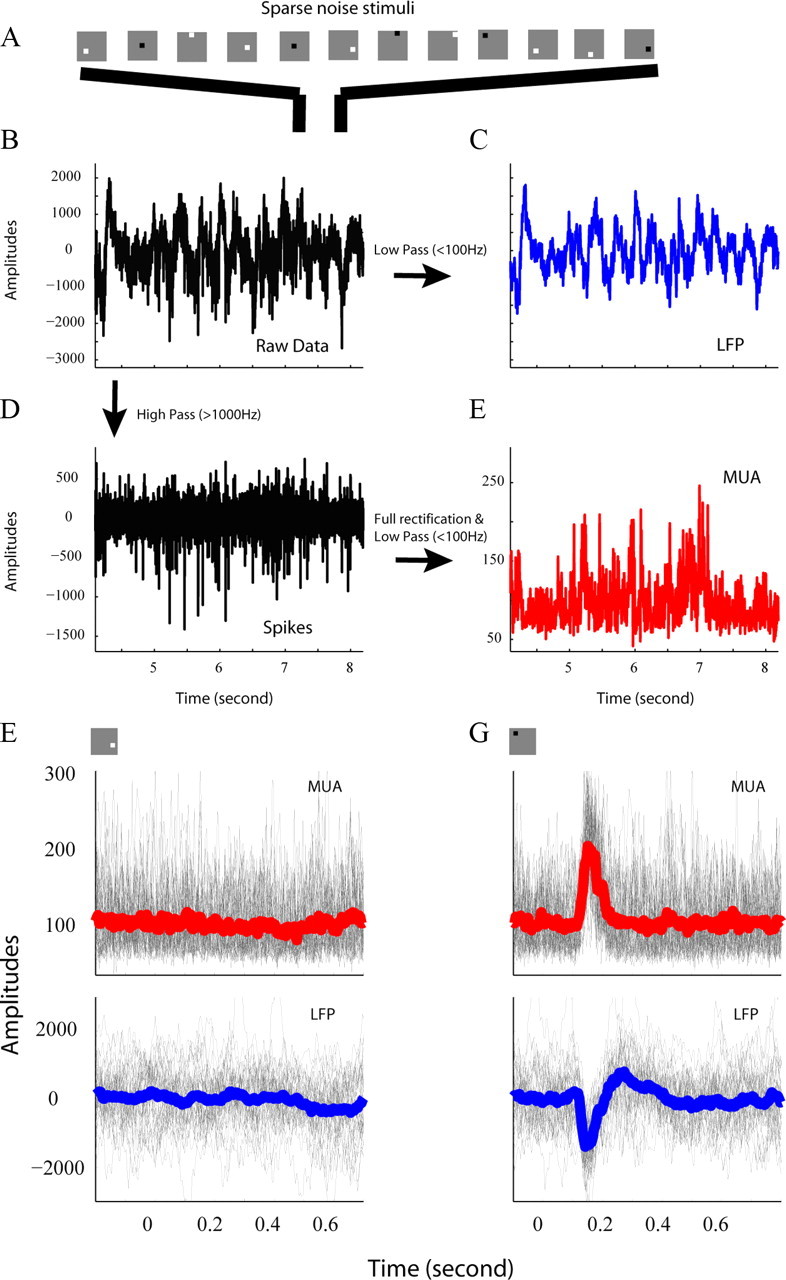
Cross-correlation between sparse noise stimuli and LFP/MUA signals. A, Each individual image in a sequence of randomly positioned (in a 12 × 12 sample grid) dark and bright squares (0.2° × 0.2°) appeared for 40 or 50 ms against a gray background. B, Unfiltered continuous signal recorded by Thomas 7-electrode system. C, Unfiltered signal in B was low-pass (100 Hz) filtered into LFP. D, High-pass-filtered (1000 Hz) raw signal contains spikes from individual neurons. E, High-passed (1000 Hz) signal then was full-wave rectified and low-pass filtered at 100 Hz, and the result was defined as MUA. F, G, LFP (top) and MUA (bottom) signals following each square type (different location and contrast polarity) were aligned by the onset of that stimulus (gray curves in F and G). Red curves in F and G are averaged traces of all MUA signals. Blue curves in F and G are averaged trace of all LFP signals.
Sparse noise mapping and visual spread map.
We used sparse noise (Jones and Palmer, 1987) to estimate the visual spreads of the LFP and MUA. The sparse noise consisted of a sequence of randomly positioned (in a 12 × 12 sample grid) (Fig. 1A) dark and bright squares (0.2° × 0.2°) against a gray background (luminance: 59.1 cd/m2). The luminance of bright and dark squares was adjusted so the contrasts from the light increment (luminance: 107.3 cd/m2) and light decrement (luminance: 11.1 cd/m2) were nearly equal. Each sparse noise image appeared for 40 or 50 ms and the entire sequence lasted ∼14 or ∼18 min (a total of 288 images, each image presented 72 times). The spatial range of all squares allowed us to measure simultaneously the visual spread maps for all recording sites from the seven electrodes. For each recording, the LFP and MUA were cross-correlated with sparse visual noise (Jones and Palmer, 1987), that is VS(x,y,τ) = 〈r(t) |S(x,y,τ − t)|〉, where x and y represent the spatial positions of pixels in the image, S(x,y,t) was the spatiotemporal visual stimulus (+1 for bright square, −1 for dark square and 0 for mean background), and r(t) was the LFP or MUA from a recording site (Fig. 1F,G).
Signal/noise ratio.
We used the signal/noise ratio of the visual spread (VS) map to determine whether or not a cell had a mappable receptive field. To define the signal/noise ratio, we calculated the spatial variance of the map (Malone et al., 2007) as σ2xy(τ) = 〈[VS(x,y,τ) − 〈VS(x,y,τ)〉]2〉x,y at two time delays: τ = 0 and τ = τpeak (τpeak of LFP is the negative peak time of the LFP at the center of the VS map and τpeak of MUA is the positive peak time of MUA at the center of the VS map) (Fig. 2C,E). The S/N ratio was then calculated as the variance at τpeak divided by the spatial variance at time 0, an estimate of the noise in the recording.
Figure 2.

Spatial-temporal Maps for LFP and MUA signals. A, LFP's dynamic responses to each stimulus pixel were plotted as blue curves in the 12 by 12 grid. LFP responses always show a negative peak (red circle in C) followed by a positive rebound (C), except for three sites in lower layer 6. Choosing positive or negative peak for the three layer 6 sites did not change our results. All amplitudes of the LFP at the time of peak negativity were plotted as a 2-D contour plot in H, representing the visual spread of LFP in 2-D visual space (defined as the VSmap). To estimate the spatial scale of the LFP, the map was projected on to x and y axes and then fitted by a 1-D Gaussian profile as illustrated in D and G respectively. B, MUA's dynamic responses to pixels at each position were plotted as red curves in each grid. Unlike the LFP, the response of MUA always had a positive peak (blue circle in E) followed by a very weak or no negative rebound (E). All amplitudes of MUA at positive peak time were plotted in a 2-D contour plot in J, which represents the visual spread of MUA in 2-D visual space (defined as the VSmap). The VSmap was projected onto x and y axes and then fitted by a Gaussian profile in F and I, respectively.
Two-dimensional visual spread for MUA and the LFP.
MUA responses at the time of peak positive response were used for the visual spread of the MUA at each site. And the LFP responses at the time of peak negative response were used for the visual spread of the LFP. The early LFP responses in the database for this study are almost always negative, except for LFPs from three sites in lower layer 6. For these three sites, choosing positive peaks or negative peaks did not affect our results.
Gaussian function fitting for visual spread of LFP and MUA.
Each VS map was fitted with a one-dimensional Gaussian function to estimate the visual spread (Fig. 2). The following is the one-dimensional Gaussian function: g(x) = exp(−(x − x0)2/(2σx)2) where variable x is the measured visual angle, and x0 and σx are respectively the center and the spatial spread of the VS map. In this paper, we only used the estimated visual spread (σvLFP and σvMUA) from the two-dimensional (2-D) map's projection on the x-axis. All results based on the projection on the y-axis are similar to that based on the x-axis (results not shown).
Model of signal summation in MUA and the LFP.
The model we developed for spatial summation in MUA and the LFP is based on the hypothesis that each signal is a sum of the electrical activity of a pool of neurons. MUA is supposed to be the sum of nerve impulse activity in the neuronal pool sampled by the recording microelectrode while the LFP is supposed to be the sum of (slow) membrane potentials. We define the visual spread of a single cortical cell to be VSSUA(y) where distance y is in units [degrees of visual angle]. We begin with the assumption that each single cell's receptive field maps precisely to a point in the visual field and each single neuron's visual spreads in terms of its spike response and membrane potential are the same (Priebe et al., 2004; Priebe and Ferster, 2005), denoted by VSSUA(y). Then equations that describe the VS maps of MUA and LFP are:
 |
 |
where gcMUA(y) and gcLFP(y) are the spatial weighting functions for cortical spatial summation of MUA and the LFP respectively, and MF is the cortical magnification factor in units of millimeters of cortex per degree of visual angle. The experimental data indicate that VSMUA(y) and VSLFP(y) are well approximated by Gaussian functions of position, so we assume that gcMUA(y) and gcLFP(y) are also Gaussians.
The data require us to revise our initial assumption about precise point-to-point mapping because the observed visual spreads VSMUA(y) and VSLFP(y) are larger than one would expect on that assumption. The simplest explanation for the larger visual spreads is scatter of the retinotopic map on the cortex (Albus, 1975). Then we need to replace the single cell spatial profile VSSUA(yi) with an average single cell profile, 〈VSSUA(yi)〉 averaged over the possible positions of the single cell spatial positions. For the sake of simplicity and computational convenience we make the approximation that the scatter is also Gaussian and therefore the average single cell signal can be approximated as:
where gVV(y) is an equivalent spatial weighting function for receptive field scatter at a point. Based on Equations 1–3, we obtain VSMUA(y) = gcMUA(MF · y) * gVV(y) * VSSUA(y) and VSLFP(y) = gcLFP(MF · y) * gVV(y) * VSSUA(y), in which all functions gcMUA, gcLFP, gVV, and VSSUA were assumed to be Gaussian functions. The Gaussian functions were used for analytical convenience because if one convolves two Gaussian functions a(y) and b(y) with spatial spread parameters σa and σb, then the result c(y) will be a Gaussian function with σc2 = σa2 + σb2. Applying this useful property to the two equations derived from Equations 1–3 we obtain:
 |
 |
where MF is the cortical magnification factor we measured in Figure 5, σvMUA and σvLFP are the visual spreads of MUA and LFP as measured in Figure 2, σvv is the spread parameter for the receptive field scatter, and σvSUA is the spread parameter for a single cell's Gaussian VS map. If one subtracts Equation 4 from Equation 5 one obtains the following:
Then the quantity we want to calculate, the spatial spread parameter for LFP signal summation in the cortex, σcLFP, is
In Equation 7, the terms σvLFP and σvMUA were derived from VS map measurements, and σcMUA, the spatial spread of multi-unit recording was estimated to lie between 30 and 100 μm based on estimates from the literature and our own experience with multi-unit recording.
Precision of estimates for parameters.
To evaluate the precision of our estimates for cortical spread of LFP, we have done simulations to obtain the bias and variation of our estimates for different pairs of σvMUA and σcLFP (50–350 μm for σcLFP; 400–700 μm for σvMUA; and 30 μm for σcMUA). For each condition, σvMUA and σcLFP -were fixed; therefore we could calculate σvLFP based on Equations 4 and 5. Then we generated Gaussian profiles of visual spread for the LFP and MUA. The spatial profiles for LFP and MUA were then sampled at a spatial resolution of 500 μm (the estimated cortical projection of the 0.2° * 0.2° dark/bright square in the experiments). We then added Gaussian noise to the down-sampled profiles. The noise level was set at 1/5 of the SD for Gaussian profile. This simulated noise level was chosen to match the Gaussian fitting error for fitting the neural data. Then σvMUA' and σvLFP' were estimated by fitting Gaussian profiles to the simulated data (note: we use the symbol x' to mean the estimated value of x). σcLFP' then was estimated from Equation 7, with the values of σvMUA' and σvLFP'. Such a procedure was repeated 35 times (35 is the number of cells for the running averages in Figs. 4 and 7), and then we calculated the mean value of the 35 σcLFP's as one estimate of the cortical spread for LFP. For each condition (a pair of σvMUA and σcLFP), we have repeated the whole procedure 1000 times to get the mean and SD of our estimate for the LFP. The simulation (supplemental Fig. 1, available at www.jneurosci.org as supplemental material) shows that, although the spatial resolution of our sample interval was 500 μm, we were able to estimate the cortical spread with a resolution of 100 μm.
Figure 4.

Visual spreads of LFP and MUA at different cortical depths. Running-averaged visual spread for the LFP and MUA are plotted as a function of cortical depth. The SEs of running-averaged visual spread for the LFP and MUA were drawn as shaded blue and red regions around corresponding running-averaged visual spreads. Running average is computed as following: for each relative cortical depth, the spread for this depth is defined as averaged spread of all recording sites within 0.1 unit of relative cortical depth.
Figure 7.

Cortical spread of LFP at different cortical depth. Running-averaged cortical spread of the LFP is plotted at different cortical depths. The solid curve was estimated by assuming that cortical spread of MUA was 60 μm and the shaded region represents the SD of the estimated cortical spread for the LFP. The running average is computed as follows: for each relative cortical depth, the spread for this depth is defined as averaged spread of all recording sites within 0.1 unit of relative cortical depth.
Histology.
Cells were assigned to different layers of V1 based on the results of track reconstruction (Hawken et al., 1988; Ringach et al., 2002). Along each track, we recorded the depths of every recording site during the experiment, and then made 3–4 electrolytic lesions at 600–900 μm intervals at the end of the experiment. A lesion was made by passing a 3 μA DC current for 2 s through the quartz platinum/tungsten microelectrodes (Thomas Recording) with a stimulus generator (ALA Scientific Instruments; model number: STG-1001). After killing, the animal was perfused through the heart with 1 L of heparinized saline (0.01 m phosphate buffered saline) followed by 2–3 L of fixative (4% paraformaldehyde, 0.25% glutaraldehyde in 0.1 m phosphate buffer). After the brain was blocked and sectioned at 0.05 mm, the lesions were initially located in unstained sections and then the lesion sections were stained for cytochrome oxidase. Cytochrome oxidase provides good anatomical localization of the laminar boundaries. Cortical layers were determined based on the cell density and cytochrome oxidase-specific labeling (Wong-Riley, 1979). After locating the lesions within the sections, we reconstructed the electrode penetration using a camera lucida, and determined the location of each recorded site relative to the reference lesions and the layers of the cortex. Our estimate of cortical depths of recording sites was quite precise: the difference between the estimated unit distance between lesion sites and the physical unit distance between two parallel electrodes (which was relatively constant across layers, e.g., tracks 2 and 3 in Fig. 6) was <5% of the average unit distance from the two measures. Therefore, factors such as the shrinkage of the brain section would not affect our estimates substantially. The mean thickness of each layer was then used to determine each cell's normalized cortical depth ranging from 0 (representing the surface) to 1 (representing the boundary between layer 6 and the white matter). The assignment of cells to layers is crucial since the cortical connectivity of different layers in the primate cortex is very different and important for their function (Rockland and Lund, 1983; Lund, 1988).
Figure 6.

Retinotopic map and magnification factor. A, Reconstruction of tracks for all seven electrodes (red lines) and recording sites (filled dots). B, VS maps of the LFP for signals simultaneously recorded from seven electrodes are shown in the upper panels as 2-D contour plots. Visual spread maps of MUA for signals simultaneously recorded from seven electrodes are shown in the lower panels as 2-D contour plots. C, VS centers of LFP (red circles) and MUA (blue circles), for seven simultaneously recorded sites, are plotted in visual field. D, Estimation of Magnification factor for the seven electrodes. Visual distance between each pair of sites is plotted on the x-axis, and cortical distance between each pair of sites is plotted on the y-axis. (red points are from the LFP map and blue points are from the MUA map).
Results
Visual spread of LFP and MUA: example
We recorded both spike activity (MUA) and field potential (LFP) with a Thomas multielectrode system in macaque V1. Data were taken from 338 recording sites in four monkeys. To estimate the cortical spread of the LFP, we used an additive model of cortical voltage summation to calculate the cortical spread of the LFP from only three physiological measures: the visual spreads of LFP and MUA (Victor et al., 1994; Gail et al., 2003) and the cortical magnification factor (MF) near the recording sites. The visual spread tells us how extensive is the region of visual space that can evoke an LFP at a recording site, while the cortical spread tells us how far the LFP from a source can propagate in the cortical tissue.
As detailed in Materials and Methods, for each recording site the simultaneously recorded responses of LFP and MUA at each location in the visual field (Fig. 2A,B) were measured by cross correlating the neural response with sparse visual noise (Jones and Palmer, 1987). The 2-D VS maps of LFP and MUA (Fig. 2H,J) were constructed by plotting the 2-D graph of the response amplitudes at their peak times (Fig. 2C,E). A VS map was called well defined on the basis of its signal/noise ratio, SNR (the criterion was SNR >1.5 for LFP and MUA; SNR = SD [VSmap when t = peak time]/SD [VSmap when t = 0]). There were 251/338 sites with well defined VS maps; this population of 251 sites forms the database for this paper.
The spatial spread of the VS map was computed by fitting a Gaussian function to horizontal (x) and vertical (y) projections of the 2-D spatial map (Fig. 2D,F,G,I), for instance along the x-axis as r = exp(−x2/(2σ)2). We defined σvLFP and σvMUA as the visual spreads of LFP and MUA.
Comparison of LFP and MUA visual spread
The visual spreads of the LFP and MUA were very similar and highly correlated (r = 0.67 in Fig. 3; means and SEs of visual spread of the LFP and MUA were: 0.263 ± 0.062°, 0.242 ± 0.049°, respectively). Therefore, independent of any further inferences, the results in Figure 3 establish that in V1 cortex visual spatial summation by the LFP signal is very similar to that of the spike activity recorded on the same microelectrode.
Figure 3.

A comparison of visual spread for the LFP and MUA. A scatter plot of visual spreads for the LFP (x-axis) and MUA (y-axis). Dashed line represents the unity line, where visual spreads for the LFP and MUA are equal.
The visual spreads of LFP and MUA depended on the cortical layer in which they were recorded (Fig. 4). Figure 4 is the first report of the laminar dependence of the visual spreads for both the LFP and MUA signals. Consistent with the graph in Figure 3, the dependence of visual spread on laminar location was very similar for the LFP and MUA. The visual spread of MUA and LFP was smallest in layer 4C. The mean difference of visual spread between layer 4C and layer 2/3 was ∼0.08° in visual angle and this interlaminar difference in visual spread was statistically significant (p < 0.001 for both LFP and MUA signals, Wilcoxon rank sum test). The layer dependence of visual spread indicates that LFP and MUA could not be signals coming from very distant locations, because otherwise there would not be such a clear laminar variation.
Model of the cortical spread of the LFP and MUA
To determine the cortical spread of the LFP, we built a schematic model to illustrate the relationship between visual spread and cortical spread of the LFP, MUA, and single-unit activity (SUA) (Fig. 5).
The minimum unit in the cortex is the individual neuron. Suppose that the LFP signal sums a pool of signals from single neurons. Then the visual spread of the LFP (σvLFP) must be the convolution of the cortical spread function of the LFP (approximated as a Gaussian function, and characterized by its spread parameter, σcLFP) and the visual spread of SUA (σvSUA). We also took into consideration another factor: σvv, the local visual variation of the locations of the visual fields of individual neurons (Albus, 1975). For simplicity, the spatial profile of visual spread, cortical spread, and visual variation were all modeled as Gaussian functions. We justify the Gaussian approximation by the goodness of fit of Gaussian functions to the VS measurements as in Figure 2. Across all recording sites, the average fractional error of the Gaussian fits to LFP and MUA maps was <0.04.
In Materials and Methods we analyze the additive model presented here and obtain a compact expression for σcLFP, the cortical spread of the LFP (from Eq. 7 in Materials and Methods), as follows: σcLFP = [MF2σvLFP2 − MF2σvMUA2 + σcMUA2]½, where σvLFP is the measured visual spread of the LFP as in Figure 2, σvMUA is the measured visual spread of MUA, and σcMUA is the cortical spread parameter of multi-unit activity. We did not measure σcMUA. However, based on the literature (Gray et al., 1995; Buzsáki, 2004) and our own experimental experience, σcMUA, the cortical spread of MUA, should not be larger than 60 μm. Because we did not know the exact cortical spread of MUA, we have used 30 and 100 μm as reasonable lower and upper bounds of MUA cortical spread. We found that such a range of MUA cortical spread did not significantly affect our estimate of the cortical spread of the LFP (data not shown). Another term in Equation 7 is MF, the cortical magnification factor. We measured MF directly with the multi-electrode matrix in the following way.
Retinotopic map and magnification factor
A critical step for the estimation of cortical spread was to estimate the MF of the cortex near our recording sites. Our seven-electrode system with microelectrodes arranged along a straight line gave us a great opportunity to estimate the cortical magnification factor precisely. For each sparse-noise experiment, we recorded simultaneously from seven cortical sites (Fig. 6A) and therefore mapped the visual spread of LFP and MUA for all seven sites simultaneously (Fig. 6B). The relative positions of VS maps for LFP and MUA (Fig. 6C) were very consistent with the relative positions of the seven sites in cortex (Fig. 6A). Distances of all site pairs in visual space were highly correlated with distances of all site pairs in the cortex (r > 0.98). For the four monkeys, the magnification factors around the cortical projection of 5° retinal eccentricity were ∼2.25–2.5 mm/deg, in good agreement with anatomical estimates (Daniel and Whitteridge, 1961; Dow et al., 1981). Based on these estimated magnification factors, the visual spreads of LFP and MUA in units of cortical distance, averaged across all sites, were: σvLFP = 622 ± 142 μm, σvMUA = 573 ± 113 μm.
Cortical spread of LFP
From calculations of cortical spread from Equation 7, we plotted the estimated cortical spread of the LFP at different cortical depths (Fig. 7) assuming the cortical spread of MUA was 60 μm (Gray et al., 1995; Buzsáki, 2004). There are two important results of our calculation of the cortical spread of the LFP: (1) the small value (∼250 μm) of the mean cortical spread of the LFP across all cortical layers; (2) a very obvious laminar variation of LFP cortical spread between layer 4B and layer 2/3. The cortical spread of the LFP is on average ∼150 μm in layer 4B and ∼280 μm in layer 2/3, and these values are significantly different (p < 0.05). Another functionally significant result is that the cortical spread of the LFP, σcLFP, is much smaller than the average visual spreads of the LFP and MUA in cortical distance, depicted in Figure 7 as the vertical blue and red lines respectively. What this means is that the spatial scale of the LFP's visual field map is not determined by σcLFP but rather by other factors. Furthermore, the relatively small value of σcLFP is one important reason why the visual spreads of MUA and LFP are so similar.
Signal/noise ratio of LFP and MUA in all layers of V1
It is also important to know how the LFP compares to the MUA as a communication signal. One way to determine this is to compare the signal/noise ratios (SNRs) of the VS maps of the two signals. A population analysis of 338 recording sites reveals that, at most sites across all layers, both LFP and MUA signals were visually driven (Fig. 8) and their SNRs were well correlated (r = 0.6). Furthermore, there was little laminar difference in the amount of visual driving (Fig. 8); there were highly responsive and weakly responsive sites in all laminae. The MUA signal consistently had a higher SNR than the LFP recorded simultaneously, as indicated by the scatter plot and also the histograms in Figure 8. These results from our dataset are consistent with the calculations of information content reported previously (Berens et al., 2008), and support the idea that the LFP in V1 carries a substantial amount of visual stimulus information though less than the MUA does.
Figure 8.

Signal to noise ratios of LFP and MUA. A, The scatter plot of LFP S/N ratio (x-axis) and MUA S/N ratio (y-axis). Vertical and horizontal dashed lines (at the value of 1.5) represent the criteria we used to determine whether a VSmap has large enough S/N ratio for LFP and MUA for the site to be considered “mappable.” The distribution of LFP S/N ratios and MUA S/N ratios are plotted in two subplots along the x and y axes of A. B, S/N ratio of the LFP was plotted as a function of cortical depth. C, S/N ratio of MUA was plotted as a function of cortical depth.
Discussion
LFP and laminar structure
How much the spatial spread of the LFP varies with location in the cortical laminae is an important and challenging question. Studies have shown that functional properties of individual neurons in different cortical layers vary substantially (Gilbert, 1977; Hawken et al., 1988; Sceniak et al., 2001; Ringach et al., 2002). However, before now it had not been determined to what extent the cortical spread of the LFP depends on cortical depth. The answer to this question provided here should significantly improve the application of the LFP to studying functional properties of the cortex and to monitoring cell populations for prostheses.
Our estimate of the laminar variation of functional properties and in particular the laminar dependence of the cortical spread of the LFP depended on the use of track reconstruction with multi-electrode recordings, and the application of our new method of relating visual to cortical spread. This new method revealed that the cortical spread of the LFP indeed varies with cortical depth in the gray matter. For example, in layer 4B the LFP on average sums from cells within a region ∼150 μm in radius around the recording electrode, while in layer 2/3, the extent of LFP signal summation is on average 280 μm.
The laminar variation of cortical spread for LFP is likely caused by layer-dependent impedance in the gray matter. Studies have shown that each layer in cortical depth has its own unique anatomical properties (Lund, 1973, 1988). This might lead to a variation of the impedance, which will determine the cortical spread of the LFP at different cortical depths. A study that directly measured the impedance of brain tissue at different cortical depths (Logothetis et al., 2007) had suggested that there might be a laminar variation of impedance in macaque V1.
In this study, we have assumed that the cortical spread of MUA is independent of cortical depth and is fixed at 60 μm. But if cortical spread for the LFP varies at different depth due to tissue impedance, the cortical spread of MUA should also vary in a similar pattern, which is: MUA spread in 2/3 is larger than that in layer 4B. This would lead to more variation of the LFP spread at different depths (based on Eq. 7). However, we think the effect of MUA spread is relatively small, because cortical spread of MUA is not the dominant term in Equation 7. We have tried estimating cortical spread of the LFP at different cortical spreads of MUA (from 30 to 100 μm), and we found the change of the LFP spread was rather small.
In addition to estimating the cortical spread of the LFP, another important question is: can the LFP represent the laminar variation of functional properties as single units can? This question, in addition to the cortical spread of the LFP, is very critical for the further application of LFP recordings, such as for neural prostheses (Andersen et al., 2004; Scherberger et al., 2005; Pesaran et al., 2006). In a given cortical area, neurons at different cortical depths usually encode different signals, and therefore their functional properties could be very different (Gilbert, 1977; Hawken et al., 1988; Sceniak et al., 2001; Ringach et al., 2002). Our results showed that one of the LFP's functional properties, the visual spread, varied across cortical laminae (Fig. 4) in a way that was highly correlated with MUA on average across cortical layers (Fig. 4) and also highly correlated site by site (Fig. 3). The implication of this result is that the LFP can be used to study laminar structure and function and can serve as the input to a neural prosthesis.
Similarity between LFP and MUA
Our results also may be relevant to the interpretation of the fMRI BOLD signal and its relation to neuronal activity in the cerebral cortex. In recent years, some experimental results on the relation between the LFP and the BOLD signal have been interpreted to mean that the dynamics of the BOLD signal are correlated with LFPs, but less correlated with neuronal spike activity (Viswanathan and Freeman, 2007). This has cast doubt on whether results from fMRI represent neuronal activity accurately. However, our study shows that LFPs in V1 cortex not only have good visual spatial resolution (Figs. 2, 6), but also the visual spreads of the spatial maps of the LFP are highly correlated, site by site, with the simultaneously recorded spatial maps of neuronal spike activity (Fig. 3). Therefore, both LFP and MUA signals give high-resolution information about the active populations of cortical neurons, and both signals are likely to be similarly correlated with the BOLD signal since they are so highly correlated with each other spatially (Fig. 3).
Model of the LFP and precision of the estimate of cortical spread
Our estimate of the average cortical spread of the LFP is similar to an estimate in layer 2/3 of cat V1 reported recently (Katzner et al., 2009) with a different approach, but is much smaller than many others'. Our result seems to contradict a number of studies (Mitzdorf, 1987; Kruse and Eckhorn, 1996; Kreiman et al., 2006; Liu and Newsome, 2006; Berens et al., 2008) that concluded that the spread of LFP signals ranges from ∼500 μm to a few millimeters. However, all such estimates rely on a model associating the LFP with functional properties of cortical neurons. For most studies (Mitzdorf, 1987; Kruse and Eckhorn, 1996; Kreiman et al., 2006; Liu and Newsome, 2006; Berens et al., 2008; Katzner et al., 2009), estimates of the cortical spread of the LFP were indirect and were associated with columnar structures of certain feature selectivities, such as orientation, direction, or speed selectivity. Because the feature selectivity of the LFP is usually broader than that of single unit activity or MUA (Kreiman et al., 2006; Liu and Newsome, 2006; Berens et al., 2008), the LFP was thought to be a signal from a cortical area wider than 500 μm. To have a precise estimate of cortical spread of the LFP in such models, one has to be very sure about what causes the feature selectivity of the LFP, a signal that probably is related to the membrane potentials of single neurons. Because of the difficulty of knowing the tuning of membrane potentials, the intracellular measure was usually replaced by extracellular measures of spikes [except in the study by Katzner et al. (2009)]. However, it is known that the feature selectivity of a cell's membrane potential is usually broader than that of spike activity (Volgushev et al., 1993; Cardin et al., 2007; Finn et al., 2007). Therefore the difference of feature selectivities between the LFP and single units probably is not completely due to wide spatial summation by the LFP.
Our estimation procedure is not as affected as others by the intracellular-extracellular tuning differences because the reverse correlation technique we used on both the LFP and on extracellular spike activity in MUA and single-unit recordings provides an estimate of underlying membrane potential tuning even for the spike activity (in our case tuning for spatial position). A more direct justification for our reverse correlation technique is from intracellular studies (Priebe et al., 2004; Priebe and Ferster, 2005). Priebe et al. (2004, 2005) have shown there is not much difference between membrane potential and spike rate maps in sparse noise mapping experiments. However, we could not rule out the possibility that some cells' visual spreads for membrane potentials were larger than those for spikes, due to a nonlinear relationship between membrane potential and spikes. To the extent that nonlinearity sharpens the spike map, it would make us overestimate the LFP cortical spread. It is also possible that the larger cortical spread in layer 2/3 might be affected by such nonlinearity. We should point out that estimates of the LFP spread by different methods are all providing an upper bound of the LFP spread. Even though we may not have avoided totally the effect of nonlinearity between spikes and membrane potentials, our estimate has set the LFP spread in a very small spatial range.
Similar to other studies, we have modeled the electrode tip as a point in space. However, a real electrode tip is more like a surface, and the size of tip exposure in principle could affect the estimate of cortical spread for the LFP. It is possible that the difference of estimation of the LFP spread is partly due to different types of electrodes used in different laboratories. However, given that the electrodes used in different laboratories can pick up well isolated single neuron spikes, we think the size difference of electrode tips is probably small. Therefore, we made the approximation that there is no practical effect of tip size on the estimated LFP spread.
In this study, we have provided a general method to estimate cortical spread of the LFP in any cortical area that has a topographic map. We were able to use the retinotopic map in V1 for this purpose. However, the key to our novel method, associating cortical space with physical space that is mapped onto the cortex, could also be used in other topographically mapped cortical areas, such as somatosensory cortex, S1. Our method does not rely on a columnar structure for feature selectivity, so it has a wider range of application than previous methods (Liu and Newsome, 2006; Katzner et al., 2009). Specifically, the method we have used for estimating the cortical spread of the LFP in macaque V1 could be extended to mouse (and other rodent) visual cortex where there is a retinotopic map but where there are no orientation columns (Hübener, 2003).
Footnotes
This work was supported by grants from the US National Science Foundation (Grant 0745253) and the US National Institutes of Health (T32 EY-07158 and R01 EY-01472) and by fellowships from the Swartz Foundation and the Robert Leet and Clara Guthrie Patterson Trust. We thank Drs. Patrick Williams and Marianne Maertens for help collecting data, and Drs. Mike Hawken, Siddhartha Joshi, and Anita Disney for advice about Histology. We would also like to thank Drs. Bijan Pesaran, Dario Ringach, and Jonathan Victor for their valuable comments and insights on this study.
References
- Albus K. A quantitative study of the projection area of the central and the paracentral visual field in area 17 of the cat. I. The precision of the topography. Exp Brain Res. 1975;24:159–179. doi: 10.1007/BF00234061. [DOI] [PubMed] [Google Scholar]
- Andersen RA, Burdick JW, Musallam S, Scherberger H, Pesaran B, Meeker D, Corneil BD, Fineman I, Nenadic Z, Branchaud E, Cham JG, Greger B, Tai YC, Mojarradi MM. Recording advances for neural prosthetics. Conf Proc IEEE Eng Med Biol Soc. 2004;7:5352–5355. doi: 10.1109/IEMBS.2004.1404494. [DOI] [PubMed] [Google Scholar]
- Berens P, Keliris GA, Ecker AS, Logothetis NK, Tolias AS. Feature selectivity of the gamma-band of the local field potential in primate primary visual cortex. Front Neurosci. 2008;2:199–207. doi: 10.3389/neuro.01.037.2008. [DOI] [PMC free article] [PubMed] [Google Scholar]
- Brosch M, Budinger E, Scheich H. Stimulus-related gamma oscillations in primate auditory cortex. J Neurophysiol. 2002;87:2715–2725. doi: 10.1152/jn.2002.87.6.2715. [DOI] [PubMed] [Google Scholar]
- Buzsáki G. Large-scale recording of neuronal ensembles. Nat Neurosci. 2004;7:446–451. doi: 10.1038/nn1233. [DOI] [PubMed] [Google Scholar]
- Cardin JA, Palmer LA, Contreras D. Stimulus feature selectivity in excitatory and inhibitory neurons in primary visual cortex. J Neurosci. 2007;27:10333–10344. doi: 10.1523/JNEUROSCI.1692-07.2007. [DOI] [PMC free article] [PubMed] [Google Scholar]
- Daniel PM, Whitteridge D. The representation of the visual field on the cerebral cortex in monkeys. J Physiol. 1961;159:203–221. doi: 10.1113/jphysiol.1961.sp006803. [DOI] [PMC free article] [PubMed] [Google Scholar]
- Dow BM, Snyder AZ, Vautin RG, Bauer R. Magnification factor and receptive field size in foveal striate cortex of the monkey. Exp Brain Res. 1981;44:213–228. doi: 10.1007/BF00237343. [DOI] [PubMed] [Google Scholar]
- Eckhorn R, Bauer R, Jordan W, Brosch M, Kruse W, Munk M, Reitboeck HJ. Coherent oscillations: a mechanism of feature linking in the visual cortex? Multiple electrode and correlation analyses in the cat. Biol Cybern. 1988;60:121–130. doi: 10.1007/BF00202899. [DOI] [PubMed] [Google Scholar]
- Finn IM, Priebe NJ, Ferster D. The emergence of contrast-invariant orientation tuning in simple cells of cat visual cortex. Neuron. 2007;54:137–152. doi: 10.1016/j.neuron.2007.02.029. [DOI] [PMC free article] [PubMed] [Google Scholar]
- Fries P, Reynolds JH, Rorie AE, Desimone R. Modulation of oscillatory neuronal synchronization by selective visual attention. Science. 2001;291:1560–1563. doi: 10.1126/science.1055465. [DOI] [PubMed] [Google Scholar]
- Gail A, Brinksmeyer HJ, Eckhorn R. Simultaneous mapping of binocular and monocular receptive fields in awake monkeys for calibrating eye alignment in a dichoptical setup. J Neurosci Methods. 2003;126:41–56. doi: 10.1016/s0165-0270(03)00067-0. [DOI] [PubMed] [Google Scholar]
- Gail A, Brinksmeyer HJ, Eckhorn R. Perception-related modulations of local field potential power and coherence in primary visual cortex of awake monkey during binocular rivalry. Cereb Cortex. 2004;14:300–313. doi: 10.1093/cercor/bhg129. [DOI] [PubMed] [Google Scholar]
- Gilbert CD. Laminar differences in receptive field properties of cells in cat primary visual cortex. J Physiol. 1977;268:391–421. doi: 10.1113/jphysiol.1977.sp011863. [DOI] [PMC free article] [PubMed] [Google Scholar]
- Goense JB, Logothetis NK. Neurophysiology of the BOLD fMRI signal in awake monkeys. Curr Biol. 2008;18:631–640. doi: 10.1016/j.cub.2008.03.054. [DOI] [PubMed] [Google Scholar]
- Gray CM, Maldonado PE, Wilson M, McNaughton B. Tetrodes markedly improve the reliability and yield of multiple single-unit isolation from multi-unit recordings in cat striate cortex. J Neurosci Methods. 1995;63:43–54. doi: 10.1016/0165-0270(95)00085-2. [DOI] [PubMed] [Google Scholar]
- Hawken MJ, Parker AJ, Lund JS. Laminar organization and contrast sensitivity of direction-selective cells in the striate cortex of the Old World monkey. J Neurosci. 1988;8:3541–3548. doi: 10.1523/JNEUROSCI.08-10-03541.1988. [DOI] [PMC free article] [PubMed] [Google Scholar]
- Henrie JA, Shapley R. LFP power spectra in V1 cortex: the graded effect of stimulus contrast. J Neurophysiol. 2005;94:479–490. doi: 10.1152/jn.00919.2004. [DOI] [PubMed] [Google Scholar]
- Hübener M. Mouse visual cortex. Curr Opin Neurobiol. 2003;13:413–420. doi: 10.1016/s0959-4388(03)00102-8. [DOI] [PubMed] [Google Scholar]
- Jones JP, Palmer LA. The two-dimensional spatial structure of simple receptive fields in cat striate cortex. J Neurophysiol. 1987;58:1187–1211. doi: 10.1152/jn.1987.58.6.1187. [DOI] [PubMed] [Google Scholar]
- Katzner S, Nauhaus I, Benucci A, Bonin V, Ringach DL, Carandini M. Local origin of field potentials in visual cortex. Neuron. 2009;61:35–41. doi: 10.1016/j.neuron.2008.11.016. [DOI] [PMC free article] [PubMed] [Google Scholar]
- Kreiman G, Hung CP, Kraskov A, Quiroga RQ, Poggio T, DiCarlo JJ. Object selectivity of local field potentials and spikes in the macaque inferior temporal cortex. Neuron. 2006;49:433–445. doi: 10.1016/j.neuron.2005.12.019. [DOI] [PubMed] [Google Scholar]
- Kruse W, Eckhorn R. Inhibition of sustained gamma oscillations (35–80 Hz) by fast transient responses in cat visual cortex. Proc Natl Acad Sci U S A. 1996;93:6112–6117. doi: 10.1073/pnas.93.12.6112. [DOI] [PMC free article] [PubMed] [Google Scholar]
- Liu J, Newsome WT. Local field potential in cortical area MT: stimulus tuning and behavioral correlations. J Neurosci. 2006;26:7779–7790. doi: 10.1523/JNEUROSCI.5052-05.2006. [DOI] [PMC free article] [PubMed] [Google Scholar]
- Logothetis NK, Pauls J, Augath M, Trinath T, Oeltermann A. Neurophysiological investigation of the basis of the fMRI signal. Nature. 2001;412:150–157. doi: 10.1038/35084005. [DOI] [PubMed] [Google Scholar]
- Logothetis NK, Kayser C, Oeltermann A. In vivo measurement of cortical impedance spectrum in monkeys: implications for signal propagation. Neuron. 2007;55:809–823. doi: 10.1016/j.neuron.2007.07.027. [DOI] [PubMed] [Google Scholar]
- Lund JS. Organization of neurons in the visual cortex, area 17, of the monkey (Macaca mulatta) J Comp Neurol. 1973;147:455–496. doi: 10.1002/cne.901470404. [DOI] [PubMed] [Google Scholar]
- Lund JS. Anatomical organization of macaque monkey striate visual cortex. Annu Rev Neurosci. 1988;11:253–288. doi: 10.1146/annurev.ne.11.030188.001345. [DOI] [PubMed] [Google Scholar]
- Malone BJ, Kumar VR, Ringach DL. Dynamics of receptive field size in primary visual cortex. J Neurophysiol. 2007;97:407–414. doi: 10.1152/jn.00830.2006. [DOI] [PubMed] [Google Scholar]
- Mitzdorf U. Properties of the evoked potential generators: current source-density analysis of visually evoked potentials in the cat cortex. Int J Neurosci. 1987;33:33–59. doi: 10.3109/00207458708985928. [DOI] [PubMed] [Google Scholar]
- Neville KR, Haberly LB. Beta and gamma oscillations in the olfactory system of the urethane-anesthetized rat. J Neurophysiol. 2003;90:3921–3930. doi: 10.1152/jn.00475.2003. [DOI] [PubMed] [Google Scholar]
- Pesaran B, Pezaris JS, Sahani M, Mitra PP, Andersen RA. Temporal structure in neuronal activity during working memory in macaque parietal cortex. Nat Neurosci. 2002;5:805–811. doi: 10.1038/nn890. [DOI] [PubMed] [Google Scholar]
- Pesaran B, Musallam S, Andersen RA. Cognitive neural prosthetics. Curr Biol. 2006;16:R77–R80. doi: 10.1016/j.cub.2006.01.043. [DOI] [PubMed] [Google Scholar]
- Pesaran B, Nelson MJ, Andersen RA. Free choice activates a decision circuit between frontal and parietal cortex. Nature. 2008;453:406–409. doi: 10.1038/nature06849. [DOI] [PMC free article] [PubMed] [Google Scholar]
- Priebe NJ, Ferster D. Direction selectivity of excitation and inhibition in simple cells of the cat primary visual cortex. Neuron. 2005;45:133–145. doi: 10.1016/j.neuron.2004.12.024. [DOI] [PubMed] [Google Scholar]
- Priebe NJ, Mechler F, Carandini M, Ferster D. The contribution of spike threshold to the dichotomy of cortical simple and complex cells. Nat Neurosci. 2004;7:1113–1122. doi: 10.1038/nn1310. [DOI] [PMC free article] [PubMed] [Google Scholar]
- Rickert J, Oliveira SC, Vaadia E, Aertsen A, Rotter S, Mehring C. Encoding of movement direction in different frequency ranges of motor cortical local field potentials. J Neurosci. 2005;25:8815–8824. doi: 10.1523/JNEUROSCI.0816-05.2005. [DOI] [PMC free article] [PubMed] [Google Scholar]
- Ringach DL, Shapley RM, Hawken MJ. Orientation selectivity in macaque V1: diversity and laminar dependence. J Neurosci. 2002;22:5639–5651. doi: 10.1523/JNEUROSCI.22-13-05639.2002. [DOI] [PMC free article] [PubMed] [Google Scholar]
- Rockland KS, Lund JS. Intrinsic laminar lattice connections in primate visual cortex. J Comp Neurol. 1983;216:303–318. doi: 10.1002/cne.902160307. [DOI] [PubMed] [Google Scholar]
- Rols G, Tallon-Baudry C, Girard P, Bertrand O, Bullier J. Cortical mapping of gamma oscillations in areas V1 and V4 of the macaque monkey. Vis Neurosci. 2001;18:527–540. doi: 10.1017/s0952523801184038. [DOI] [PubMed] [Google Scholar]
- Sceniak MP, Hawken MJ, Shapley R. Visual spatial characterization of macaque V1 neurons. J Neurophysiol. 2001;85:1873–1887. doi: 10.1152/jn.2001.85.5.1873. [DOI] [PubMed] [Google Scholar]
- Scherberger H, Jarvis MR, Andersen RA. Cortical local field potential encodes movement intentions in the posterior parietal cortex. Neuron. 2005;46:347–354. doi: 10.1016/j.neuron.2005.03.004. [DOI] [PubMed] [Google Scholar]
- Sirota A, Montgomery S, Fujisawa S, Isomura Y, Zugaro M, Buzsáki G. Entrainment of neocortical neurons and gamma oscillations by the hippocampal theta rhythm. Neuron. 2008;60:683–697. doi: 10.1016/j.neuron.2008.09.014. [DOI] [PMC free article] [PubMed] [Google Scholar]
- Victor JD, Purpura K, Katz E, Mao B. Population encoding of spatial frequency, orientation, and color in macaque V1. J Neurophysiol. 1994;72:2151–2166. doi: 10.1152/jn.1994.72.5.2151. [DOI] [PubMed] [Google Scholar]
- Viswanathan A, Freeman RD. Neurometabolic coupling in cerebral cortex reflects synaptic more than spiking activity. Nat Neurosci. 2007;10:1308–1312. doi: 10.1038/nn1977. [DOI] [PubMed] [Google Scholar]
- Volgushev M, Pei X, Vidyasagar TR, Creutzfeldt OD. Excitation and inhibition in orientation selectivity of cat visual cortex neurons revealed by whole-cell recordings in vivo. Vis Neurosci. 1993;10:1151–1155. doi: 10.1017/s0952523800010257. [DOI] [PubMed] [Google Scholar]
- Womelsdorf T, Fries P, Mitra PP, Desimone R. Gamma-band synchronization in visual cortex predicts speed of change detection. Nature. 2006;439:733–736. doi: 10.1038/nature04258. [DOI] [PubMed] [Google Scholar]
- Wong-Riley M. Columnar cortico-cortical interconnections within the visual system of the squirrel and macaque monkeys. Brain Res. 1979;162:201–217. doi: 10.1016/0006-8993(79)90284-1. [DOI] [PubMed] [Google Scholar]