

Abstract
Near-Poisson variability in auditory-nerve (AN) responses limits the accuracy of automated tuning-curve algorithms. Here, a typical adaptive tuning-curve algorithm was used with a physiologically realistic AN model with and without the inclusion of neural randomness. Response randomness produced variability in Q10 estimates that was nearly as large as in AN data. Results suggest that it is sufficient for AN models to specify frequency selectivity based on mean Q10 values at each characteristic frequency (CF). Errors in estimates of CF, which decreased from ±0.2 octaves at low frequencies to ±0.05 octaves at high frequencies, are significant for studies of spatiotemporal coding.
1. Introduction
Automated tuning-curve algorithms have been used for many years to characterize the tuning properties of auditory-nerve (AN) fibers (Liberman, 1978; Miller et al., 1997; Heinz and Young, 2004). The sound pressure level necessary to increase the AN response to a 50-ms tone by a small criteria (typically 1 spike) is determined as a function of tone frequency in order to map the threshold tuning curve. The near-Poisson variability of AN responses limits the accuracy with which individual thresholds can be estimated quickly. For example, empirical data suggest that a standard deviation of 1.25 spikes is expected within a 50-ms window for a fiber with an overall discharge rate of 50 spikes/ s (Young and Barta, 1986; Winter and Palmer, 1991). Thus, a typical high spontaneous-rate (SR) fiber has a standard deviation that is larger than the typical criterion used to estimate threshold. Adaptive tracking procedures are used as an efficient method to estimate thresholds given the random nature of AN responses. However, the relatively short holding time for AN-fiber recordings requires a compromise between an adaptive algorithm with great accuracy and one that is quick enough to allow other stimuli of interest to be presented.
Given the necessarily quick nature of the automated algorithms, there is some amount of variability in parameters that are estimated from tuning curves. Characteristic frequency [(CF) the frequency to which a fiber responds to the lowest sound level], fiber threshold (the threshold sound level at CF), and Q10 (a measure of sharpness of tuning equal to the ratio of CF to the bandwidth 10 dB above threshold) are typical parameters derived from tuning curves. Population plots of thresholds and Q10 values derived from tuning curves typically show a range of values at each CF (e.g., Liberman, 1978; Miller et al., 1997). Although much of the variability in threshold arises from the dependence of threshold on SR, thresholds for individual fibers have been shown to differ from thresholds estimated from rate-level functions by ±10 dB (Liberman, 1978). The observed variability in Q10 values has provided a challenge to AN modeling studies because AN fibers with similar CF and different Q10 values would be expected to show somewhat different responses to complex stimuli, such as vowels (Bruce et al., 2003). However, it is possible that much of the Q10 variation observed in the data may simply be due to variability in Q10 estimates derived from automated tuning-curve algorithms. Finally, although it is not apparent in typical AN-fiber population plots, there is also likely to be variability in estimates of CF. Although such variability may be insignificant for single-fiber response properties, there has been a long-standing interest in spatiotemporal coding mechanisms that rely on the relative temporal patterns across AN fibers with slightly different CFs (Shamma, 1985; Deng and Geisler, 1987; Heinz et al., 2001; Carney et al., 2002; Cedolin and Delgutte, 2007; Heinz, 2007). Such across-CF mechanisms have a strong parametric dependence on the CF difference between AN fibers and this parameter will have a variability that is roughly twice as large as the variability in individual CF estimates. Thus, it is also important to examine the precision with which CF is estimated from typical automated tuning-curve algorithms.
2. Methods
2.1 Auditory-nerve model
The AN model described by Zilany and Bruce (2006) was used in this study. This phenomenological AN model represents an extension of several previous versions of the AN model that have been extensively tested against physiological responses to both simple and complex stimuli, including tones, two-tone complexes, broadband noise, and speech (Zhang et al., 2001; Bruce et al., 2003). Important for the purposes of the present study, the model has been fit well to tuning curves and to the statistical properties of AN responses. Tuning-curve parameters derived from the model were shown to match very well with those derived from neurophysiological data collected from cats (Miller et al., 1997). Model thresholds match well across CF to the lowest thresholds from the cat data, whereas Q10 values derived from model tuning curves fit well with the 50th percentile of the Q10 data from cats as a function of CF. The statistics of AN responses are represented in the model by using the time-varying discharge rate waveform as the driving function to a nonhomogeneous Poisson process, which has been modified to include both absolute and relative refractory effects. Although this Poisson-based model does not capture all of the detailed stochastic properties of AN fiber activity (e.g., Heil et al., 2007), the main statistical properties that are most relevant to the present study are well represented by this model (e.g., Young and Barta, 1986).
In the present study, tuning curves were measured based on outputs at two different model stages to evaluate the effect of randomness on tuning-curve estimates. To include the neural variability associated with AN responses, tuning curves were first measured based on the spike outputs of the model. To remove the effects of randomness (and refractoriness), model tuning curves were also measured based on the time-varying discharge rate waveforms prior to the generation of spikes. Note that this version of the model contains all other response properties, including the adaptation associated with synaptic transmission. Because of the adaptive nature of the tuning-curve algorithm, separate tuning curves had to be derived for each of these cases. All model simulations are for high-SR fibers and are based on the SR value (50 spikes/ s) for which this AN model was designed and tested (Zilany and Bruce, 2006).
2.2 Automated tuning-curve algorithm
The adaptive algorithm used here has been used in numerous experimental studies to measure frequency threshold tuning curves of AN fibers (e.g., Liberman, 1978; Miller et al., 1997; Heinz and Young, 2004). This algorithm, which is described in detail by Liberman (1978), represents an efficient method to track the threshold sound level necessary to elicit a small increase in AN-fiber response as a function of frequency. At each frequency, the number of spikes occurring in the final 50 ms of a 60-ms tone (with 5-ms rise/fall ramps) is compared to the number of spikes occurring in the final 50 ms of the 60-ms window following the offset of the tone. If the difference is larger than a specified criterion (0 spikes here), then the sound level is decreased by one step (2 dB), otherwise the sound level is raised by two steps (4 dB). Tone bursts are presented every 120 ms and the sound level is tracked adaptively until a threshold is determined for the current frequency. Threshold is determined when a specified pattern of tracked sound levels is observed for the current frequency; specifically the current sound level must be (1) equal to the sound level three and six steps previous in the track and (2) a decrease from the previous level. This pattern indicates that the current sound level is a reasonable estimate of the threshold level needed to increase the rate by 0–20 spikes/ s based on a criterion of 0 spikes (Liberman, 1978). Between 20 and 35 frequencies per octave are used, depending on the expected CF. The three parameters CF, threshold, and Q10 are estimated from each tuning curve, following five-point triangular smoothing (consistent with Miller et al., 1997, see their Fig. 8).
2.3 Neurophysiological recordings
Repeated measures of tuning curves were collected for three AN fibers during two experiments that were part of other studies in the lab. Single-unit AN responses were measured from chinchillas, weighing 400–600 g, using standard techniques (Heinz and Young, 2004) that were approved by the Purdue Animal Use and Care Committee. Animals were anesthetized initially with xylazine (0.5–1 mg/kg im) and ketamine (40–50 mg/kg im). Supplemental doses of sodium pentobarbital (~10 mg/h iv) were given to maintain an areflexic state of anesthesia throughout the experiment. A tracheotomy was performed to allow a low-resistance airway. The bulla was vented with PE tubing to equalize the middle-ear pressure. The animal’s rectal temperature was maintained near 37.5 °C with a feedback heating pad. A craniotomy was made in the posterior fossa to expose the cerebellum that overlies the auditory-nerve/cochlear-nucleus complex. AN-fiber recordings were made by inserting a 15–30 MΩ glass micropipette filled with 3M NaCl into the AN under visual control after aspiration of the overlying cerebellum. Recordings were made in an electrically shielded, double-walled sound-proofed room, and computer-controlled stimuli were presented via a calibrated closed-field acoustic system. Isolated fibers were characterized by the automated tuning-curve algorithm described earlier. Spontaneous rate was estimated from the off-time of a CF-tone rate-level function. Between 5 and 11 repeated tuning curves were recorded from each AN fiber depending on the holding time.
3. Results
Figure 1 illustrates the effect of AN response variability on individual tuning curves estimated from a single modelAN fiber. Figure 1(A) shows the resulting tuning curve as measured by the adaptive algorithm when the effects of randomness were excluded from the AN model. For comparison, Fig. 1(B) shows a tuning curve measured when the effects of randomness were included in the AN model. Note that the individual data points, which represent the thresholds obtained at each frequency from the adaptive algorithm, are extremely orderly in the non-random case and are quite variable when randomness was included in the model. The smoothed curve (as typically used with experimental data), eliminates much of the variability in the random case; however, some differences are still apparent. Figure 1(C) shows five repeated tuning curves using the same AN model CF with randomness included and illustrates the extent of variability across repeated measures. The derived parameter estimates from the five repeated measures of the tuning curve are listed in the figure caption. The CFs ranged from 1.97 to 2.08 kHz (a 0.08-octave range), thresholds ranged from 0.7 to 2.7 dB SPL, and Q10 values ranged from 3.0 to 4.6. Thus, even with the typical smoothing applied to the tuning curve data, variability remains in each of the parameters. Note that the range of estimated thresholds was 6–8 dB higher in the random case than the nonrandom case, whereas the range of Q10 and CF estimates with randomness surrounded the values obtained without randomness.
Fig. 1.
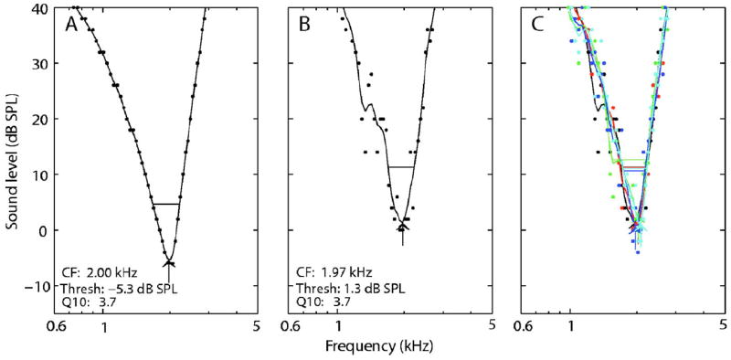
(Color online) Tuning curves measured by the adaptive algorithm with and without randomness for an AN-model fiber with CF = 2.0 kHz and SR = 50 spikes/ s. (A) AN model without randomness. Individual data points represent the thresholds estimated by the adaptive algorithm at each frequency. Solid lines represent a smoothed curve (see the text). Identical tuning curves were obtained with repeated measures. (B) AN model with randomness. (C) Five repeated tuning curves with randomness. Derived parameters for the individual repetitions are: CF (kHz) = 1.97,2.02,2.02,1.97,2.08; geometric mean = 2.01; and range = 0.08 octaves. Threshold (dB SPL) = 1.3,1.3,2.7,0.7,1.1; mean = 1.4; range = 2.0 dB. Q10 = 3.7,3.7,3.0,4.6,4.2; geo. mean = 3.8; range=0.62 octaves. The information may not be properly conveyed in black and white.
The effects of randomness on population estimates of threshold and Q10 values are illustrated in Figs. 2(A) and 2(B). Tuning curves were measured from model AN fibers with nominal CFs spaced logarithmically from 0.3 to 10 kHz. Red lines in Figs. 2(A) and 2(B) shows results when randomness was excluded from the AN model and blue symbols show derived parameters when randomness was included. In the nonrandom case [red lines, Fig. 2(A)], model thresholds were consistent with those reported by Zilany and Bruce (2006), ranging down to −5 dB SPL between 1 and 2 kHz and showing an increase at low frequencies and near 4 kHz based on the cat middle-ear filter. The inclusion of randomness [symbols, Fig. 2(A)] produced thresholds that were consistently higher than the nonrandom case and that spanned a range of about 10 dB in each CF region. This variation was not seen in the non-random case. The derived Q10 values in the nonrandom case [red lines, Fig. 2(B)] showed an increasing trend with CF that matched the mean of the physiological data (Miller et al., 1997), but showed little variability in each CF region (except for the 4–5 kHz region corresponding to the middle-ear notch). When randomness was included [symbols, Fig. 2(B)], an increasing trend across CF was observed with large variability within each CF region. Predicted Q10 values spanned much of the 5th–95th percentile range (dashed lines) of Q10 values measured from cats (Miller et al., 1997). Note that the Q10 variability spans above and below the nonrandom Q10 values, unlike the threshold estimates that were consistently above the nonrandom values.
Fig. 2.
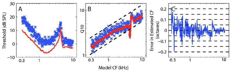
(Color online) (A) Populations of thresholds, (B) Q10 values, and (C) CF errors estimated from tuning curves measured for 250 model AN fibers. (A and B) Each symbol (X) represents the estimated value with randomness and red lines represent nonrandom estimates. (B) Black dashed lines represent the range between the 5th and 95th percentile of experimental Q10 values within each CF region (Miller et al., 1997). (C) Error in estimated CFs from tuning curves measured when randomness was included. CF error in octaves is computed as log2 (estimated CF/model CF). The information in (A) and (B) may not be properly conveyed in black and white.
The effect of neural randomness on the variability in tuning-curve estimates of CF is shown in Fig. 2(C). The error in the CF estimates for the 250 tuning curves that were included in Figs. 2(A) and 2(B) is plotted as a function of the model CF. Although the errors are centered around zero, i.e., tuning-curve estimates are essentially unbiased, there is a range of errors at all model CFs. The largest errors are observed at the lowest CFs (0.3–0.4 kHz), where errors fall within a ±0.2-octave range. For mid CF values (0.7–2.0 kHz), errors generally fall within a ±0.1-octave range. At the highest CFs, errors are restricted to within a ±0.05-octave range, with the exception of the region surrounding 4 kHz. The cat middle-ear transfer function has a sharp notch in gain (of almost 20 dB) centered between 4 and 5 kHz (Bruce et al., 2003), which creates a sharp increase in CF thresholds near 4 kHz [Fig. 2(A)]. This sharp gain reduction leads to slightly biased CF estimates and larger errors at model CFs surrounding the notch. Note that the bias is in opposite directions above and below the center frequency of the notch, with CFs below the notch having CF estimates that are biased downwards and CFs above the notch having an upward bias. Overall, the observation of larger octave errors at lower CFs is consistent with shallower tuning curves (lower Q10 values) having a less-well defined CF, for which alternative estimates of CF based on spike timing have been proposed (Joris et al., 2006).
The general model predictions were tested by measuring repeated tuning curves for several AN fibers recorded from chinchillas. Figure 3 shows the variability across repeated tuning curves for three AN fibers ranging in CF and SR. The variability in estimated tuning-curve parameters for each fiber is listed in the figure caption, along with the SR values. The qualitative variability in tuning-curve shape was larger for the high-SR fibers [Figs. 3(A) and 3(B)] as compared to the fiber with lower SR [Fig. 3(C)]. This resulted in less variability in threshold and Q10 estimates for the lower-SR fiber. However, the range of CF estimates was largest for the lower-SR fiber (0.14 octaves) because of its low CF, consistent with the model predictions shown in Fig. 2(C). The ranges of CF estimates for the three AN fibers (0.08–0.14 octaves) are quantitatively consistent with the modeling predictions shown in Fig. 2(C).
Fig. 3.
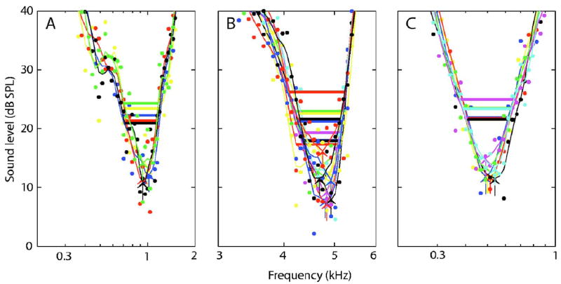
(Color online) Repeated tuning curves measured from three AN fibers from chinchillas, which vary in SR and CF. Derived parameters for the individual repetitions are: (A: SR = 58.8 spikes/ s) CF (kHz) = 1.00,1.00,0.96,0.96,0.93; geometric mean = 0.97; range = 0.11 octaves. Threshold (dB SPL) = 13.4,12.3,11.4,10.9,14.3; mean = 12.5; range = 3.4. Q10 = 2.3,1.9,2.4,2.2, 2.0; geo. mean = 2.2; range = 0.34 octs. (B: SR = 54.6) CF = 4.75, 4.75,4.84,4.93,4.66,4.84,4.93,4.93,4.93,4.75,4.66; geo. mean = 4.78; range = 0.08 octs. Threshold = 11.5,8.0,7.3,7.9,12.9,9.3,11.5,12.6,11.2,16.2,11.6; mean = 9.5; range = 5.6. Q10 = 4.4,5.9,5.5,6.0,4.5,5.7,6.1,4.9,5.4,4.1,5.6; geo. mean = 5.2; range = 0.45 octs. (C: SR = 3.7) CF = 0.50,0.49, 0.51,0.54,0.49,0.49,0.54; geo. mean = 0.51; range = 0.14 octs. Threshold = 11.5,11.9,11.7,11.5,13.4,15.0,13.3; mean = 12.0; range = 1.9. Q10 = 2.2,2.4,2.3,2.1,2.0,1.7,2.2; geo. mean = 2.2; range = 0.26 octs. The information may not be properly conveyed in black and white.
4. Discussion
The modeling and experimental results presented here are based on one specific automated tuning-curve algorithm; however, the effects shown are likely to play a significant role in the variability observed in tuning-curve estimates derived from other techniques as well, including nonadaptive methods (e.g., Kiang et al., 1965; Evans, 1972). The modeling results shown in Fig. 2(B) suggest that the variability observed in Q10 values derived from experimental AN data is largely due to the effects of response variability on the precision of Q10 estimates derived from tuning curves. The Q10 values derived from the AN model without randomness fell in the middle of the range of Q10 values derived from the model with randomness. This results suggests that it is sufficient for AN models to fit frequency selectivity based on the 50th percentile of Q10 values at each CF (Bruce et al., 2003; Zilany and Bruce, 2006). It does not appear to be necessary to assume that different AN fibers with similar CFs have inherently different frequency selectivity. The finding that the range of threshold estimates was above the nonrandom threshold, while the variability in Q10 estimates ranged above and below the nonrandom case supports the typical interpretation of such data (e.g., Miller et al., 1997; Bruce et al., 2003).
The range of errors in CF estimates was shown to decrease from ±0.2 octaves at low frequencies to ±0.05 octaves at high frequencies. These errors appear to be quite small, consistent with the qualitative impression that the automated algorithm provides a reasonably consistent estimate of frequency selectivity across repeated tuning-curve measurements [Figs. 1(C) and 3(A)–3(C)]. This degree of variability in CF estimates may be adequate for most population studies, including those that quantify rate-place coding (e.g., Sachs and Young, 1979) and those that quantify temporal-place coding in terms of metrics that depend on the average magnitude of phase locking within a range of CFs [e.g., the average localized synchronized rate (ALSR) (Young and Sachs, 1979)]. However, the variability in CF estimates is significant for studies of spatiotemporal coding that depend on the relative phase response across nearby CFs (e.g., Shamma, 1985; Palmer, 1990). This is because narrow cochlear filters have sharp phase transitions near CF that translate a small error in CF into a large phase shift. For example, two AN fibers with CFs surrounding (±0.05 octaves) a vowel formant at 1 kHz are predicted to have a 1/4-cycle phase difference between their phase-locked responses (Heinz, 2007). The model predictions in Fig. 3 suggest that CF estimates near 1 kHz could be in error by up to ±0.1 octaves, implying that the estimate of CF difference could be in error by up to ±0.2 octaves. Given the sharp phase transition, a 0.4-octave range in CF difference corresponds to a ±1/2-cycle range in phase shift. The large effect of small CF errors on spatiotemporal response patterns is likely to be why it has been hard to study spatiotemporal cues quantitatively with experimental data (e.g., Palmer, 1990), and why many spatiotemporal studies have used models where the CF difference is controllable (Deng and Geisler, 1987; Heinz et al., 2001; Carney et al., 2002). The limitations imposed by the variability in CF estimates for spatiotemporal coding studies can be overcome by techniques that predict the response of a population of AN fibers with similar CFs responding to a single stimulus from the response of a single AN fiber responding to frequency-shifted stimuli (Cedolin and Delgutte, 2007; Heinz, 2007).
Acknowledgments
The authors thank Ian Bruce for initial discussions and suggestions related to evaluating the variability in experimental Q10 values. Thanks are also given to Ian Bruce, Sushrut Kale, and Jayaganesh Swaminathan for providing valuable comments on a previous version of the manuscript. Special thanks are given to Sushrut Kale for his help with collection of the neurophysiological AN data. This research was supported by NIH-NIDCD.
Contributor Information
Ananthakrishna Chintanpalli, Weldon School of Biomedical Engineering, Purdue University, 206 S. Martin Jischke Drive, West Lafayette, Indiana 47907, cananthk@purdue.edu.
Michael G. Heinz, Department of Speech, Language and Hearing Sciences and Weldon School of Biomedical Engineering, Purdue University, 500 Oval Drive, West Lafayette, Indiana 47907, mheinz@purdue.edu
References and links
- Bruce IC, Sachs MB, Young ED. An auditory-periphery model of the effects of acoustic trauma on auditory nerve responses. J Acoust Soc Am. 2003;113:369–388. doi: 10.1121/1.1519544. [DOI] [PubMed] [Google Scholar]
- Carney LH, Heinz MG, Evilsizer ME, Gilkey RH, Colburn HS. Auditory phase opponency: A temporal model for masked detection at low frequencies. Acust Acta Acust. 2002;88:334–347. [Google Scholar]
- Cedolin L, Delgutte B. Spatio-temporal representation of the pitch of complex tones in the auditory nerve. In: Kollmeier B, Klump G, Hohmann V, Langemann U, Mauermann M, Uppenkamp S, Verhey J, editors. Hearing–From Sensory Processing to Perception. Springer; Berlin: 2007. pp. 61–70. [Google Scholar]
- Deng L, Geisler CD. A composite auditory model for processing speech sounds. J Acoust Soc Am. 1987;82:2001–2012. doi: 10.1121/1.395644. [DOI] [PubMed] [Google Scholar]
- Evans EF. The frequency response and other properties of single fibres in the guinea-pig cochlear nerve. J Physiol. 1972;226:263–287. doi: 10.1113/jphysiol.1972.sp009984. [DOI] [PMC free article] [PubMed] [Google Scholar]
- Heil P, Neubauer H, Irvine DR, Brown M. Spontaneous activity of auditory-nerve fibers: Insights into stochastic processes at ribbon synapses. J Neurosci. 2007;27:8457–8474. doi: 10.1523/JNEUROSCI.1512-07.2007. [DOI] [PMC free article] [PubMed] [Google Scholar]
- Heinz MG. Spatiotemporal encoding of vowels in noise studied with the responses of individual auditory nerve fibers. In: Kollmeier B, Klump G, Hohmann V, Langemann U, Mauermann M, Uppenkamp S, Verhey J, editors. Hearing–From Sensory Processing to Perception. Springer-Verlag; Berlin: 2007. pp. 107–115. [Google Scholar]
- Heinz MG, Colburn HS, Carney LH. Rate and timing cues associated with the cochlear amplifier: Level discrimination based on monaural cross-frequency coincidence detection. J Acoust Soc Am. 2001;110:2065–2084. doi: 10.1121/1.1404977. [DOI] [PubMed] [Google Scholar]
- Heinz MG, Young ED. Response growth with sound level in auditory-nerve fibers after noise-induced hearing loss. J Neurophysiol. 2004;91:784–795. doi: 10.1152/jn.00776.2003. [DOI] [PMC free article] [PubMed] [Google Scholar]
- Joris PX, Van de Sande B, Louage DH, van der Heijden M. Binaural and cochlear disparities. Proc Natl Acad Sci U S A. 2006;103:12917–12922. doi: 10.1073/pnas.0601396103. [DOI] [PMC free article] [PubMed] [Google Scholar]
- Kiang NYS, Watanabe T, Thomas EC, Clark LF. Discharge Patterns of Single Fibers in the Cat’s Auditory Nerve. MIT Press; Cambridge, MA: 1965. [Google Scholar]
- Liberman MC. Auditory-nerve response from cats raised in a low-noise chamber. J Acoust Soc Am. 1978;63:442–455. doi: 10.1121/1.381736. [DOI] [PubMed] [Google Scholar]
- Miller RL, Schilling JR, Franck KR, Young ED. Effects of acoustic trauma on the representation of the vowel /ε/ in cat auditory nerve fibers. J Acoust Soc Am. 1997;101:3602–3616. doi: 10.1121/1.418321. [DOI] [PubMed] [Google Scholar]
- Palmer AR. The representation of the spectra and fundamental frequencies of steady-state single- and double-vowel sounds in the temporal discharge patterns of guinea pig cochlear-nerve fibers. J Acoust Soc Am. 1990;88:1412–1426. doi: 10.1121/1.400329. [DOI] [PubMed] [Google Scholar]
- Sachs MB, Young ED. Encoding of steady-state vowels in the auditory nerve: Representation in terms of discharge rate. J Acoust Soc Am. 1979;66:470–479. doi: 10.1121/1.383098. [DOI] [PubMed] [Google Scholar]
- Shamma SA. Speech processing in the auditory system. I: The representation of speech sounds in the responses of the auditory nerve. J Acoust Soc Am. 1985;78:1612–1621. doi: 10.1121/1.392799. [DOI] [PubMed] [Google Scholar]
- Winter IM, Palmer AR. Intensity coding in low-frequency auditory-nerve fibers of the guinea pig. J Acoust Soc Am. 1991;90:1958–1967. doi: 10.1121/1.401675. [DOI] [PubMed] [Google Scholar]
- Young ED, Barta PE. Rate responses of auditory nerve fibers to tones in noise near masked threshold. J Acoust Soc Am. 1986;79:426–442. doi: 10.1121/1.393530. [DOI] [PubMed] [Google Scholar]
- Young ED, Sachs MB. Representation of steady-state vowels in the temporal aspects of the discharge patterns of populations of auditory-nerve fibers. J Acoust Soc Am. 1979;66:1381–1403. doi: 10.1121/1.383532. [DOI] [PubMed] [Google Scholar]
- Zhang X, Heinz MG, Bruce IC, Carney LH. A phenomenological model for the responses of auditory-nerve fibers: I. Nonlinear tuning with compression and suppression. J Acoust Soc Am. 2001;109:648–670. doi: 10.1121/1.1336503. [DOI] [PubMed] [Google Scholar]
- Zilany MSA, Bruce IC. Modeling auditory-nerve responses for high sound pressure levels in the normal and impaired auditory periphery. J Acoust Soc Am. 2006;120:1446–1466. doi: 10.1121/1.2225512. [DOI] [PubMed] [Google Scholar]