Quadratic Regularization Design for 2D CT

Abstract

Statistical methods for tomographic image reconstruction have improved noise and spatial resolution properties that may improve image quality in X-ray CT. Penalized weighted least squares (PWLS) methods using conventional quadratic regularization lead to nonuniform and anisotropic spatial resolution due to interactions between the weighting, which is necessary for good noise properties, and the regularizer. Previously, we addressed this problem for parallel-beam emission tomography using matrix algebra methods to design data-dependent, shift-variant regularizers that improve resolution uniformity. This paper develops a fast Angular Integral Mostly Analytical, AIMA, regularization design method for 2D fan-beam X-ray CT imaging, for which parallel-beam tomography is a special case. Simulation results demonstrate that the new method for regularization design requires very modest computation and leads to nearly uniform and isotropic spatial resolution in transmission tomography when using quadratic regularization.

I. Introduction

Statistical image reconstruction methods for X-ray Computed Tomography (CT) imaging have the potential to reduce patient dose, reduce artifacts from beam hardening and metal objects, and accommodate scanning geometries that are poorly suited for conventional FBP reconstruction. Unregularized image reconstruction leads to excessively noisy images, which necessitates noise control such as a penalized weighted least squares¹ (PWLS) method, or a penalized-likelihood (PL) method [1].

Although PL and PWLS methods can control noise, interactions between a conventional quadratic roughness penalty and the weighting that is explicit in PWLS methods [2], and is implicit in PL methods, results in images with nonuniform and anisotropic spatial resolution, even for idealized shift-invariant imaging systems [3]. Fan-beam geometries used in X-ray CT are shift-variant and contain additional variations in spatial resolution over the field of view (FOV) [4]. The resulting non-uniformities and anisotropy could be avoided in part by using a conventional penalized unweighted least-squares (PULS) estimation method. However without the weighting, PULS yields poor noise properties (akin to FBP).

Much previous work on regularization design focuses on matrix-based approaches to fit the local impulse response of the estimator to a target impulse response. A shift-variant regularizer based on the aggregate certainty of measurement rays intersecting each pixel was developed that yielded uniform but anisotropic spatial resolution [3]. Stayman parameterized the quadratic regularizer to produce uniform and isotropic spatial resolution [5] and generalized regularization design to other non-Poisson noise models [6]. [7] presents a regularization design method for uniform and isotropic spatial resolution that is not based on an explicit target point spread function (PSF), but rather focuses on circular symmetry and uniformity. Extensions to 3D PET have also been proposed [8], [9].

We previously proposed an analytical approach to regularization design for 2D parallel-beam emission reconstruction that uses continuous space analogs to simplify the regularization design problem [10]. This paper extends [10] by developing a mostly analytical approach to regularization design for fan-beam geometries [11]. §II reviews the concept of a local impulse response (LIR) and discusses the design of regularizers that yield approximately uniform and isotropic spatial resolution. §III uses the frequency domain to gain some insight into the problem and derives a minimization problem to solve for the appropriate regularization coefficients. §IV describes efficient techniques for computing the regularization coefficients. §V presents the results of our simulations using simulated and real X-ray CT data, and §VI analyzes them.

II. Local Impulse Reponse

Let y = (y₁, …, y_M) denote the vector of noisy transmission sinogram measurements recorded in a CT system. For simplicity, we consider the following mono-energetic formulation for the ensemble mean of the measured data:

$${\overline{y}}_{\mathit{\text{i}}}(\mathit{x})=E[y_{\mathit{\text{i}}}]=b_{\mathit{\text{i}}}{e}^{-{[\mathit{\text{Ax}}]}_{\mathit{\text{i}}}}+r_{\mathit{\text{i}}},$$ (1)

where A is the system matrix, x = (x₁, x₂, …, x_N) is a discretized version of the object being imaged, b_i denotes the blank scan, r_i denotes the additive contribution of scatter, and ${[\mathit{\text{Ax}}]}_{\mathit{\text{i}}}={\sum }_{j=1}^N{a}_{\mathit{\text{i}}j}{x}_j$. The spatial resolution and therefore regularization design techniques are applicable to PL methods when appropriate weightings are chosen [3]. We estimate x by minimizing the following cost function:

$$\Psi (\mathit{\text{y}},\mathit{\text{x}})\triangleq {\Vert \ell (\mathit{\text{y}})-\mathit{\text{Ax}}\Vert }_{\mathit{\text{W}}}^2+\zeta \text{R}(\mathit{x})$$ (2)

$$\widehat{\mathit{\text{x}}}(\mathit{\text{y}})=\underset{\mathit{\text{x}}}{\text{arg}min}\Phi (\mathit{\text{y}},\mathit{x}),$$ (3)

where $\ell (\mathit{\text{y}})\triangleq -\text{ln}\left(\frac{\mathit{\text{y}}-\mathit{\text{r}}}{\mathit{\text{b}}}\right)$ using element-wise division, R(x) is a regularizer that controls noise, ζ is a scalar that determines the resolution-noise tradeoff, and W = diag{w_i} is a statistical weighting matrix. For transmission tomography with the model in (1), usually we have the plug-in weighting w_i = y_i corresponding to the PL estimator for (1) [12]. For emission tomography, the plug-in weighting is w_i = 1/y_i; for low count levels alternative weightings are preferable [13]. The regularization design methods in this paper apply to other statistical models than (1) by simply changing the weighting matrix W.

The goal of this work is to design R(x) so that the reconstructed image has approximately uniform and isotropic spatial resolution. The tools developed for this purpose could be modified to achieve other resolution design goals. Analyzing the local impulse response (LIR) is an essential part of assessing the resolution. Here we use the following definition of local impulse response for the jth pixel:

$$\begin{array}{ll}{\mathit{\text{l}}}^j\hfill & \triangleq \underset{\epsilon \to 0}{lim}\frac{\widehat{\mathit{\text{x}}}(\overline{\mathit{\text{y}}}({\mathit{\text{x}}}_{\text{true}}+\epsilon {\mathit{\delta }}^j))-\widehat{\mathit{\text{x}}}(\overline{\mathit{\text{y}}}({\mathit{\text{x}}}_{\text{true}}))}{\epsilon }\hfill \\ \hfill & ={\nabla }_{\mathit{\text{y}}}\widehat{\mathit{\text{x}}}(\mathit{y}){|}_{\mathit{y}=\overline{\mathit{y}}({\mathit{\text{x}}}_{\text{true}})}{\nabla }_{\mathit{\text{x}}}\overline{\mathit{y}}(\mathit{x}){|}_{\mathit{x}={\mathit{x}}_{\text{true}}}{\mathit{\delta }}^j,\hfill \end{array}$$ (4)

where δ^j is a Kronecker impulse at the jth pixel and the gradient operations are matrices such that ${[{\nabla }_{\mathit{\text{y}}}\widehat{\mathit{x}}(\mathit{\text{y}})]}_{j\mathit{\text{i}}}=\frac{\partial }{\partial {\text{y}}_{\mathit{\text{i}}}}{\widehat{x}}_j(\mathit{y})$ and ${[{\nabla }_{\mathit{\text{x}}}\overline{\mathit{y}}(\mathit{\text{x}})]}_{\mathit{\text{i}}j}=\frac{\partial }{\partial {\text{x}}_j}{\overline{y}}_{\mathit{\text{i}}}(\mathit{x})$ (this definition depends on the mean of the data, rather than the mean of x̂ and differs slightly from that used in [3], but yields the same final expression without requiring further approximations). Evaluating (4) [3], the LIR for the PWLS estimator (3) is

$${\mathit{\text{l}}}^j={\mathit{\text{l}}}^j({\mathit{\text{x}}}_{\text{true}},\mathit{\text{R}})={[\mathit{\text{A}}\prime \mathit{\text{W A}}+\zeta \mathit{\text{R}}]}^{-1}\mathit{\text{A}}\prime \mathit{\text{W A}}{\mathit{\delta }}^j,$$ (5)

where R is the Hessian of the regularizer R(x).

As is evident from (5), the local impulse response depends on the regularizer through its Hessian, R. We would like to design R such that the local impulse response l^j best matches a target response l⁰ at every pixel j. We could phrase this matrix optimization problem as:

$$\underset{\mathit{\text{R}}}{\text{arg}min}\sum _{\text{j}}{\Vert {\mathit{\text{S}}}^j{\mathit{\text{l}}}^j({\mathit{\text{x}}}_{\text{true}},\mathit{\text{R}})-{\mathit{\text{l}}}^0\Vert }^2,$$ (6)

where S^j is a shift operator that recenters l^j to the center pixel. This matrix formulation of the design problem seems intractable, so we turn to the frequency domain to simplify the problem.

III. Frequency Domain Analysis

This section first reviews the use of discrete Fourier transforms for resolution analysis, leading to a computationally intensive approach to regularization design. We then consider continuous-space analogs that lead to simplified designs.

A. Discrete Fourier Analysis

An analytical expression for A′W Aδ^j is derived in Appendix §B, showing that A′W Aδ^j changes slowly with j. Thus A′W A is approximately locally circulant. The R matrix in (5) can be designed to be locally circulant as well. This allows us to factor out a Fourier transform matrix in (5).

Let Q denote an orthonormal discrete Fourier transform matrix centered at pixel j (we recenter the Fourier matrix to avoid the complex exponentials caused by non-centered impulse responses). Then A′W A ≈ Q′ Λ^j Q, where ${\mathbf{\Lambda }}^j=\text{diag}\left\{{\lambda }_k^{\mathit{\text{j}}}\right\}$ and λ^j ≜ F(A′W Aδ^j), and R ≈ Q′Γ^jQ, where ${\mathbf{\Gamma }}^j=\text{diag}\left\{{\gamma }_{\mathit{\text{k}}}^j\right\}$ and γ^j ≜ F(Rδ^j), where F(·) denotes the 2D DFT [8], [14]. Then we can approximate the LIR in (5) as:

$${\mathit{\text{l}}}^j\approx {\left[\mathit{\text{Q}}\prime {\mathbf{\Lambda }}^j\mathit{\text{Q}}+\zeta \mathit{\text{Q}}\prime {\mathbf{\Gamma }}^j\mathit{\text{Q}}\right]}^{-1}\mathit{\text{Q}}\prime {\mathbf{\Lambda }}^j\mathit{\text{Q}}{\mathit{\delta }}^j$$ (7)

$$={\mathit{\text{Q}}}^{\prime }\left[\frac{{\mathbf{\Lambda }}^j}{{\mathbf{\Lambda }}^j+\zeta {\mathbf{\Gamma }}^j}\right]\mathit{Q}{\mathit{\delta }}^j,$$ (8)

where the matrices in the bracketed term are diagonal and the division operation is element-wise on the diagonal. These approximations are accurate only for row and column indices that are “sufficiently close” to pixel j. The terms in brackets in (8) correspond to the local frequency response of our estimator. We would like to match these to the frequency response L⁰ of a target PSF (that will be discussed in §III-B) as closely as possible, i.e., we want

$${\mathit{\text{L}}}^j\triangleq \frac{{\mathbf{\Lambda }}^j}{{\mathbf{\Lambda }}^j+\zeta {\mathbf{\Gamma }}^j}\approx {\mathit{\text{L}}}^0.$$ (9)

Based on (9), one might consider a DFT formulation of the regularization design using the following minimization approach:

$${\widehat{\mathbf{\Gamma }}}^j=\underset{\Gamma \in \mathcal{T}}{\text{arg}min}\Vert {\mathit{L}}^0-\frac{{\mathbf{\Lambda }}^j}{{\mathbf{\Lambda }}^j+\zeta {\mathbf{\Gamma }}^j}\Vert ,$$ (10)

where L⁰ is the frequency response of l⁰ and denotes the set of possible frequency responses for the regularizer limited by its structure that will be enumerated in §III-B. Alternatively, as a preview of the methods in §IV-A, we can cross multiply the terms in (9) yielding the simpler design criterion:

$${\widehat{\mathbf{\Gamma }}}^{\text{j}}=\underset{\Gamma \in \mathcal{T}}{\text{arg}min}\Vert {\mathit{L}}^0({\mathbf{\Lambda }}^{\text{j}}+\zeta {\mathbf{\Gamma }}^j)-{\mathbf{\Lambda }}^j\Vert .$$ (11)

This approach is similar to the formulation in [6]. Because Λ^j is the DFT of A′W Aδ^j, calculating Λ^j requires one forward projection and backward projection per pixel. Thus, regularization design based on (10) or (11) would be very slow.

Prior to [10], regularization design methods were based on discrete Fourier transforms. As shown in Appendix B, the continuous-space analog of Λ^j in polar coordinates (ρ, Φ) is the frequency response $\frac{w^{\mathit{\text{j}}}(\Phi )}{\left|\rho \right|}$, where w^j(Φ) is an expression that incorporates the Jacobian from the change of coordinates from parallel-beam to fan-beam geometry, and weights from W that correspond to rays that intersect pixel j at angle Φ. Substituting this into (9) and using continuous space analogs of Γ^j yields the following expression for the continuous space analog of L^j:

$$\begin{array}{ll}{ℒ}^{\mathit{\text{j}}}(\rho ,\Phi )\hfill & \approx \frac{w^{\mathit{\text{j}}}(\Phi )\frac{1}{\left|\rho \right|}}{w^{\mathit{\text{j}}}(\Phi )\frac{1}{\left|\rho \right|}+\zeta R^{\mathit{\text{j}}}(\rho ,\Phi )}\hfill \\ \hfill & =\frac{w^{\mathit{\text{j}}}(\Phi )}{w^{\mathit{\text{j}}}(\Phi )+\zeta \left|\rho \right|R^j(\rho ,\Phi )},\hfill \end{array}$$ (12)

where R^j(ρ, Φ) is the local frequency response of the regularizer near pixel j. The continuous space analogs of Λ^j and Γ^j simplify (12) to provide a more efficient approach to regularization design than (11), as detailed below in (27).

B. Regularization Structure

Regularizers control roughness by penalizing differences between neighboring pixels. Indexing the image x as a 2D function x(n, m), we define a first-order differencing function for a regularizer that penalizes the lth direction as

$$c_l(n,m)=\frac{1}{\sqrt{n_{\mathit{\text{l}}}^2+m_{\mathit{\text{l}}}^2}}(\delta (n,m)-\delta (n-n_{\mathit{\text{l}}},m-m_{\mathit{\text{l}}})),$$ (13)

where typically (n_l, m_l) ∈ {(0, 1), (1, 0), (1, 1), (−1, 1)}, corresponding to horizontal, vertical, and diagonal differences. A conventional quadratic regularizer can then be expressed as

$$R(\mathit{\text{x}})=\sum _{n,m}\sum _{l=1}^L\frac{1}{2}{\left|(c_{\mathit{\text{l}}}\ast \ast x)(n,m)\right|}^2,$$ (14)

where ** denotes 2D convolution. This conventional regularizer assigns the same weight to the differences between each neighbor. In this paper, we make the regularizer spatially adaptive with the addition of weighting coefficients $r_{\mathit{\text{l}}}^j$ as follows:

$$R(\mathit{\text{x}})=\sum _{n,m}\sum _{l=1}^L{r}_{\mathit{\text{l}}}^j\frac{1}{2}{\left|(c_{\mathit{\text{l}}}\ast \ast x)(n,m)\right|}^2,$$ (15)

where j is the columnized pixel index which is a function of (n, m). The objective of this paper is to design coefficients $\left\{r_{\mathit{\text{l}}}^j\right\}$. To this end, we must analyze the local frequency response R^j(ρ, Φ) of the Hessian R of the space-variant regularizer (15).

Taking the Fourier transform of (13) yields:

$$\begin{array}{cc}|C_{\mathit{\text{l}}}({\omega }_1,{\omega }_2){|}^2\hfill & =\frac{1}{n_{\mathit{\text{l}}}^2+m_{\mathit{\text{l}}}^2}|1-e^{-\mathit{\text{i}}({\omega }_1{n}_{\mathit{\text{l}}}+{\omega }_2{m}_{\mathit{\text{l}}})}{|}^2\\ & =\frac{1}{n_{\mathit{\text{l}}}^2+m_{\mathit{\text{l}}}^2}(2-2cos({\omega }_1,n_{\mathit{\text{l}}}+{\omega }_2,m_{\mathit{\text{l}}}).\hfill \end{array}$$ (16)

Combining (16) and (15) yields an accurate expression for the local frequency response of our regularizer that leads to the slower but more accurate Full Integral Iterative NNLS, FIIN, method, described in Appendix §A. Next we use an approximation to simplify (16) that will lead to a fast, Angular Integral Mostly Analytical, AIMA method.

C. Efficient Approximation for R

Using the approximation 2 − 2 cos(x) ≈ x², which we will refer to as the AIMA approximation, (16) simplifies to

$${\left|C_{\mathit{\text{l}}}({\omega }_1,{\omega }_2)\right|}^2\approx \frac{1}{n_{\mathit{\text{l}}}^2+m_{\mathit{\text{l}}}^2}{({\omega }_1{n}_{\mathit{\text{l}}}+{\omega }_2{m}_{\mathit{\text{l}}})}^2.$$ (17)

One can think about isotropy intuitively in polar coordinates as eliminating angular dependence. Therefore we convert (17) to polar frequency coordinates to simplify the analysis. Using frequency and sampling relationships from the DFT, ω₁ = 2πΔ_xρ cos(Φ) and ω₂ = 2πΔ_yρ sin(Φ), where Δ_x, Δ_y denotes pixel size and (ρ, Φ) are polar frequency coordinates. For simplicity, we assume Δ_x = Δ_y = 1 for square pixels. Then:

$$\begin{array}{ll}{\left|C_{\mathit{\text{l}}}({\omega }_1,{\omega }_2)\right|}^2\hfill & \approx \hfill \\ \hfill & \frac{1}{n_{\mathit{\text{l}}}^2+m_{\mathit{\text{l}}}^2}{(n_{\mathit{\text{l}}}2\pi {\Delta }_x\rho cos(\Phi )+m_{\mathit{\text{l}}}2\pi {\Delta }_y\rho sin(\Phi ))}^2\hfill \\ \hfill & =\frac{1}{n_{\mathit{\text{l}}}^2+m_{\mathit{\text{l}}}^2}{(2\pi \rho )}^2{(n_{\mathit{\text{l}}}cos(\Phi )+m_{\mathit{\text{l}}}sin(\Phi ))}^2\hfill \\ \hfill & ={(2\pi \rho )}^2{cos}^2(\Phi -{\Phi }_l),\hfill \end{array}$$ (18)

where ${\Phi }_l\triangleq {tan}^{-1}\frac{m_{\mathit{\text{l}}}}{n_{\mathit{\text{l}}}}$. Taking the Fourier transform of (15) and combining with (18), our final expression for the local frequency response of the regularizer near the jth pixel is

$$R^{\mathit{\text{j}}}(\rho ,\Phi )=\sum _{l=1}^L{r}_{\mathit{\text{l}}}^j{(2\pi \rho )}^2{cos}^2(\Phi -{\Phi }_l).$$ (19)

For the usual choice of L = 4 and for (n_l, m_l) described below (13), Φ_l ∈ {0, π/2, π/4, 3π/4}.

D. Target Local Frequency Response

Substituting (19) into (12) yields a simple expression for the local frequency response of a PWLS estimator. We want to design each regularization coefficient vector ${\mathit{\text{r}}}^j=(r_1^j,\dots ,r_{\mathit{\text{L}}}^j)$ such that our frequency response matches that of the target as closely as possible. We know that the local frequency response associated with PULS is isotropic at the center of the field of view so we select that to be our target.

Using (n_l, m_l) ∈ {(0, 1), (1, 0)}, the squared magnitude response of a conventional regularizer in (14) using the AIMA approximation is,

$$R_0(\rho ,\Phi )={(2\pi \rho )}^2$$ (20)

and without the approximation is

$$R_0(\rho ,\Phi )=4-2cos(2\pi \rho cos\Phi )-2sin(2\pi \rho sin\Phi ).$$ (21)

For an unweighted cost function and a parallel beam geometry, the continuous-space frequency response that is analogous to F(A′ Aδ^j) is $\frac{1}{|\mathit{\rho }|}$. As shown in (49) in Appendix §B, for uniform weights (w_i = 1) we have the following local frequency response for fan-beam geometries

$$H^j(\rho ,\Phi )=\frac{2}{J(s^j(\Phi ))\left|\rho \right|},$$ (22)

where J(s^j(Φ)) is the Jacobian for the change of coordinates from parallel-beam to fan-beam geometries as defined in (44), and s^j(Φ) is an index into the sinogram based on pixel j and angle Φ. Setting s^j(Φ) = 0 to correspond with the center pixel in (49), the target local frequency response is:

$${ℒ}^0\triangleq \frac{\frac{2}{J(0)\left|\rho \right|}}{\frac{2}{J(0)\left|\rho \right|}+\zeta R_0(\rho ,\Phi )}$$ (23)

$$=\frac{1}{1+\zeta \left|\rho \right|0.5J(0)R_0(\rho ,\Phi )},$$ (24)

where ⁰ is the continuous-space analog of L⁰ in (9). Next we will use these continuous-space analogs to solve for the regularization coefficients r^j.

IV. The AIMA Approach

This section describes the Angular Integral Mostly Analytical, AIMA, approach. This approach is appropriately named because the continuous space approximations removes all dependence on ρ leaving a single integral over the angular coordinate Φ. This also results in a very simple problem that can be solved mostly analytically.

A. Solving for regularization coefficients

We try to design regularization coefficients r^j to match our designed local frequency response (12) to the target local frequency response (24) as follows:

$$\frac{w^{\mathit{\text{j}}}(\Phi )}{w^{\mathit{\text{j}}}(\Phi )+\zeta \left|\rho \right|R^{\mathit{\text{j}}}(\rho ,\Phi )}\approx \frac{1}{1+\zeta \left|\rho \right|0.5J(0){(2\pi \rho )}^2}.$$ (25)

Cross multiplying and simplifying yields

$$\begin{array}{c}{w}^{\mathit{\text{j}}}(\Phi )\zeta \left|\rho \right|0.5J(0){(2\pi \rho )}^2\approx \zeta \left|\rho \right|R^{\mathit{\text{j}}}(\rho ,\Phi )\hfill \\ w^{\mathit{\text{j}}}(\Phi )0.5J(0){(2\pi \rho )}^2\approx \sum _{l=1}^L{r}_{\mathit{\text{l}}}^j{(2\pi \rho )}^2{cos}^2(\Phi -{\Phi }_l)\hfill \\ {\stackrel{\sim }{w}}^j(\Phi )\triangleq w^{\mathit{\text{j}}}(\Phi )0.5J(0)\approx \sum _{l=1}^L{r}_{\mathit{\text{l}}}^j{cos}^2(\Phi -{\Phi }_l).\hfill \end{array}$$ (26)

We design r^j by minimizing the difference between both sides of (26):

$${\mathit{r}}^{\mathit{\text{j}}}=\underset{\mathit{\text{r}}\ge 0}{\text{arg}min}\frac{1}{2\pi }{{\int }_0^{2\pi }\left({\stackrel{\sim }{w}}^j(\Phi )-\sum _{l=1}^L{r}_l{cos}^2(\Phi -{\Phi }_l)\right)}^{2}d\Phi .$$ (27)

We solve for L coefficients using the above minimization for each pixel j. We constrain the L coefficients to be non-negative which ensures that the penalty function is convex. This expression also applies to parallel-beam geometries, where J(0) = 1.

We can think of the minimization in (27) as a projection of w̃^j = (Φ) onto the space spanned by {cos²(− Φ_l)}, which allows us to greatly simplify the problem and derive a computationally efficient and mostly analytical solution to the regularization design problem. Expanding these cosines in terms of a three term basis that is orthonormal with respect to the inner product $\langle f,g\rangle =\frac{1}{2\pi }{\int }_0^{2\pi }f(\Phi )g(\Phi )d\Phi$ yields

$${cos}^2(\Phi -{\Phi }_l)=\frac{1}{2}\cdot 1+\frac{cos(2{\Phi }_l)}{2\sqrt{2}}\left[\sqrt{2}cos(2\Phi )\right]+\frac{sin(2{\Phi }_l)}{2\sqrt{2}}\left[\sqrt{2}sin(2\Phi )\right].$$ (28)

The three orthonormal basis functions are

$$\begin{array}{l}{p}_1(\Phi )=1\\ p_2(\Phi )=\sqrt{2}cos(2\Phi )\\ p_3(\Phi )=\sqrt{2}sin(2\Phi ).\end{array}$$

Using (27), we write ${\sum }_{l=1}^L{r}_{\mathit{\text{l}}}^j{cos}^2(\Phi -{\Phi }_l)={\mathit{\text{PTr}}}^j$, where P is an operator whose columns are p₁, p₂, and p₃, and T is a 3 × L matrix of linear combination coefficients whose lth column is ${\left[\frac{1}{2}\frac{cos(2{\Phi }_l)}{2\sqrt{2}}\frac{sin(2{\Phi }_l)}{2\sqrt{2}}\right]}^T.$. T is computed by taking the inner products of cos²(Φ − Φ_l) and p₁, p₂, and p₃, i.e., T_mn = ∫ cos²(Φ − Φ_m) p_n(Φ)dΦ.

Using (28), the minimization problem (27) simplifies to the following expression:

$${\mathit{\text{r}}}^j=\underset{\mathit{\text{r}}\ge 0}{\text{arg}min}{\Vert \mathit{\text{Tr}}-{\mathit{\text{b}}}^j\Vert }^2,$$ (29)

where b^j ≜ P*w̃^j (·) and P* denotes the adjoint of P, i.e., $b_{\mathit{\text{k}}}^j=\int p_{\mathit{\text{k}}}(\Phi ){\stackrel{\sim }{w}}^j(\Phi )d\Phi$, k = 1, 2, 3.

B. Zeros in the Hessian

If there are too many zeros in r^j, there will be zeros in the Hessian, possibly degrading x̂. This can cause elongated impulse responses that may contribute to streak artifacts in the reconstructed image. This phenomenon occurred in [10] however we did not notice the artifacts due to the coarser spatial resolution in PET. It is present when using AIMA with the ring phantom in §V. The problem improves when using FIIN method of §A, thus we believe this phenomenon is caused by the approximation error in (17) as well as the non-negativity constraint. For AIMA, and to be safe using FIIN, we modify (29) to ensure that an adequate number of $r_{\mathit{\text{l}}}^j$ values are greater than some ${\epsilon }_{\mathit{\text{l}}}^j>0$. Requiring the penalty coefficients for the vertical and horizontal directions be nonzero is sufficient to eliminate zeros in the Hessian. (A similar constraint could be created using the 2 diagonals instead of the vertical and horizontal neighbors; however the approximation in (17) is worse for diagonal neighbors). We turn to previous work to select ${\epsilon }_{\mathit{\text{l}}}^j$. In [3], we derived a certainty based weighting using a spatially variant ${({\kappa }^j)}^2=\frac{{\sum }_{\mathit{\text{i}}}{a}_{\mathit{\text{i}}j}^2{\stackrel{\sim }{w}}_{\mathit{\text{i}}}}{{\sum }_{\mathit{\text{i}}}{a}_{\mathit{\text{i}}j}^2}$ that seeks to provide uniform spatial resolution. In terms of the continuous space analogs used in this paper, ${({\kappa }^{\mathit{\text{j}}})}^2=\frac{1}{\pi }{\int }_0^{\pi }{\stackrel{\sim }{w}}^j(\Phi )d\Phi$. This regularization design method can be implemented using the regularization structure presented in this paper by setting $r_{\mathit{\text{l}}}^j={({\kappa }^{\mathit{\text{j}}})}^2$ for (m_l, n_l) = (0, 1), (1, 0). This approach provides a convenient nominal value for the regularization strength at each pixel. We define the lower constraint vector ε^j such that ${\epsilon }_{\mathit{\text{l}}}^j=\alpha {({\kappa }^{\mathit{\text{j}}})}^2$ for vertical and horizontal neighbors, (m_l, n_l) = (0, 1), (1, 0), and ${\epsilon }_{\mathit{\text{l}}}^j=0$ for all other neighbors. Using a nonzero coefficient α improves noise at the expense of isotropy. For the results presented in this paper, we used α = 0.1.

Now we formulate our problem so that non-negative least squares (NNLS) algorithms will accommodate this new constraint. Let r̄^j ≜ r^j + ε^j. Solving with the constraint of r^j ≥ 0 ensures that r̄^j ≥ ε^j. Substituting r̄^j into (29) yields Tr̄^j − b^j = T(r^j + ε^j) − b^j = Tr^j − (b^j − Tε^j). So our final cost function for regularization design is

$$\begin{array}{ll}{\widehat{\mathit{\text{r}}}}^j\hfill & =\underset{\mathit{r}\ge 0}{\text{arg}min}\Vert \mathit{\text{Tr}}-({\mathit{\text{b}}}^j-\mathit{\text{T}}{\mathit{\epsilon }}^j)\Vert \hfill \\ \hfill & =\underset{\mathit{r}\ge 0}{\text{arg}min}\Vert \mathit{\text{Tr}}-{\overline{\mathit{b}}}^j\Vert ,\hfill \end{array}$$ (30)

where b̄^j ≜ b^j − Tε^j. We use coefficients r̄^j = r̂^j + ε^j in the regularizer (15). We next solve (30) analytically. It is this analytical solution that makes the AIMA more efficient than the FIIN method of Appendix §A.

C. A Mostly Analytical Solution

Using a second-order neighborhood (L = 4) we select (n_l, m_l) to be (1, 0), (0, 1), (1, 1), (1, −1) leading to the following Φ_l: Φ₁ = 0, Φ₂ = π/2, Φ₃ = π/4, Φ₄ = −π/4. So the terms in (30) are

$$\begin{array}{c}\mathit{\text{T}}=\frac{1}{2}\left[\begin{array}{cccc}\hfill 1\hfill & \hfill 1\hfill & \hfill 1\hfill & \hfill 1\hfill \\ \hfill 1/\sqrt{2}\hfill & \hfill -1/\sqrt{2}\hfill & \hfill 0\hfill & \hfill 0\hfill \\ \hfill 0\hfill & \hfill 0\hfill & \hfill 1/\sqrt{2}\hfill & \hfill -1/\sqrt{2}\hfill \end{array}\right]\\ {\overline{\mathit{\text{b}}}}^{\text{j}}=\left[\begin{array}{c}{\text{d}}_1^{\text{j}}\\ \sqrt{2}{d}_2^j\\ \sqrt{2}{d}_3^j\end{array}\right],d^{\mathit{\text{j}}}=\left[\begin{array}{c}\frac{1}{2\pi }(1-\alpha ){\int }_0^{2\pi }{\stackrel{\sim }{w}}^j(\Phi )d\Phi \\ \frac{1}{2\pi }{\int }_0^{2\pi }{\stackrel{\sim }{w}}^j(\Phi )cos(2\Phi )d\Phi \\ \frac{1}{2\pi }{\int }_0^{2\pi }{\stackrel{\sim }{w}}^j(\Phi )sin(2\Phi )d\Phi \end{array}\right].\end{array}$$ (31)

Observe that Tε^j = [α(κ^j)² 0 0]^T, so ε^j affects only d₁. Ignoring α, d₁ is the continuous space analog of the certainty-based regularization weighting in [3], d₂ is related to the horizontal and vertical directions, and d₃ is related to the diagonal directions.

The system (31) is under-determined, which is somewhat intuitive since one can obtain approximately isotropic smoothing using only the horizontal and vertical neighbors, or only the diagonal neighbors. For the purposes of regularization design, an under-determined situation is desirable since it allows us to use the “extra” degrees of freedom to ensure non-negativity even when anisotropic regularization is needed.

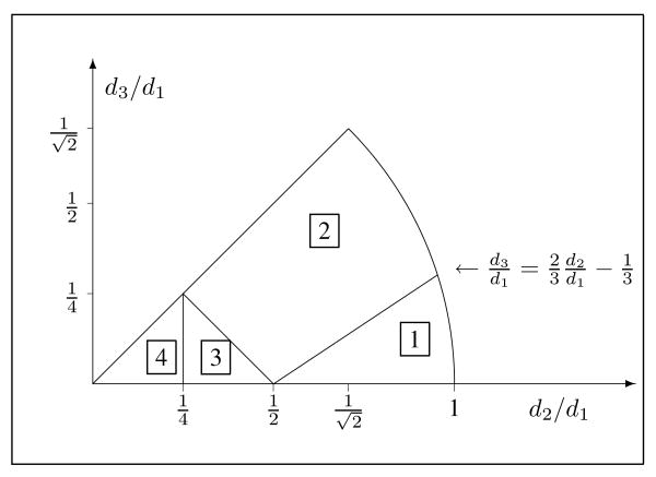
We could solve the minimization (30) using an iterative NNLS algorithm [15, p. 158]. However, using the properties of T and d, we can avoid iterations almost entirely by solving (30) analytically using the KKT conditions. When α = 0, $\sqrt{d_2^2+d_3^2}\le d_1$. as outlined in Appendix C. This inequality is usually true for the values of α used (typically around 0.1), however for pixels where it is not, the problem would have to be solved using a NNLS algorithm rather than this analytical solution. To use NNLS, one must add Tikhonov regularization to help (30) converge to a minimum norm solution which ensures that r^j is a continuous function of d^j which is a continuous function of w̃^j(Φ). For more details on using NNLS to solve the regularization problem, see §IV-A in [9]. For the results presented in this paper, all pixels of both simulations satisfie $\sqrt{d_2^2+d_3^2}\le d_1$ for all pixels and NNLS was not used. The structure of T leads to eight-fold symmetry that simplifies analysis. If d₂ < 0 we can solve for r using |d₂| and then swap r₁ with r₂. If d₃ < 0 we can solve for r using |d₃| and then swap r₃ with r₄. If d₃ > d₂ we can solve for r with d₂ and d₃ interchanged, and then swap r₁ with r₃ and r₂ with r₄. Therefore, hereafter we focus on cases where 0 ≤ d₃ ≤ d₂ ≤ d₁. Fig. 1 shows these first octant cases, numbered according to the number of nonzero elements of r.

Fig. 1.

First octant of quadratic penalty design space showing the four regions where different constraints are active.

1. If $d_2\ge \frac{1}{2}{d}_1$ and $d_3\le \frac{2}{3}{d}_2-\frac{1}{3}{d}_1$, then $r_1=\frac{4}{3}\left(d_1+d_2\right)$, r₂ = r₃ = r₄ = 0.

2. If $d_3\ge \frac{2}{3}{d}_2-\frac{1}{3}{d}_1$ and $d_3+d_2\ge \frac{1}{2}{d}_1$, then $r_1=\frac{8}{5}\left[\frac{1}{2}{d}_1+\frac{3}{2}{d}_2-d_3\right]$, r₂ = r₄ = 0, $r_3=\frac{12}{5}\left[d_3-\left(\frac{2}{3}{d}_2-\frac{1}{3}{d}_1\right)\right]$.

3. If $d_3+d_2\le \frac{1}{2}{d}_1$ and $d_2\ge \frac{1}{4}{d}_1$, then there are multiple non-negative r that exactly solve ∇Ψ(r) = 0. The minimum-norm solution is r₁ = 4d₂, r₂ = 0,

   r₃ = d₁ − 2d₂ + 2d₃, $r_4=2\left[\frac{1}{2}{d}_1-(d_2+d_3)\right]$.

4. If $d_2\le \frac{1}{4}{d}_1$, then there are multiple non-negative r that are exact solutions. The natural choice is the minimum-norm r given by the pseudo-inverse solution r = T^†d, where $r_1=2\left(\frac{1}{4}{d}_1+d_2\right)$, $r_2=2\left(\frac{1}{4}{d}_1-d_2\right)$, $r_3=2\left(\frac{1}{4}{d}_1+d_3\right)$, $r_4=2\left(\frac{1}{4}{d}_1-d_3\right)$.

The analytical solution presented above is for the usual first-order differences (13). For higher-order differences or neighborhoods, it would appear to become increasingly cumbersome to solve (27) analytically, so an iterative NNLS approach may be more appealing. This can still be practical since T is quite small. The analytical solution above is a continuous function of d, which in turn is a continuous function of w̃^j(Φ). This continuity property would seem to be desirable for avoiding artifacts in the reconstructed images.

For practical implementation, we simply discretize the integrals in (31) [16]. This presents interpolation issues in extracting a discretized version of w̃^j(Φ), from W. For the fan beam case, we use the analytical formula for w̃^j(Φ) presented in Appendix §B (48). Those equations are presented with continuous space coordinates s that spans the length of the detector, and β, the angle of rotation of the system. In discrete implementation, we round these off to the nearest neighbor to get indices into W. The analytical solution presented in this section is very efficient over all values of j, and the bulk of the computation time is spent computing w̃^j(Φ) which has the compute time of approximately one back-projection. For further speed optimizations, down-sampled back-projections could be explored. In practice, w̃^j(Φ) is fairly smooth and the basis functions that we use to approximate w̃^j(Φ) are even smoother. One can achieve good results by calculating w̃^j(Φ) for fewer angles and interpolating the rest. The performance and efficacy of such a scheme still needs to be explored.

V. Results

We first investigated imaging a phantom consisting of two uniform rings that highlight the effects of non-uniformities and anisotropy [7]. Afterwards, we studied real CT data.

We simulated a 2D 3rd-generation fan-beam CT system using distance-driven forward and backprojections [17]. The rotation center is 40.8cm from the detector, and the source is 94.9cm from the detector. The axis of rotation is at the center of the object. The simulated imaging system has 888 rays per view spaced 1mm apart, and 984 evenly spaced view angles over a 2π rotation. The reconstructed images consisted of a 512 × 512 grid of 1 mm pixels. We chose a ζ in (24) such that the target PSF has a full width half max (FWHM) of 3.18 mm.

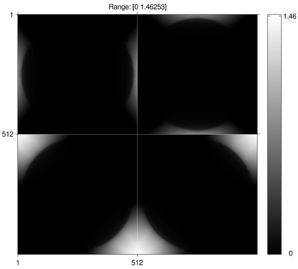
We simulated a noiseless fan-beam sinogram without scatter using a phantom consisting of a background disk and two rings each of thickness 1mm shown in Fig. 2. We generated the noiseless sinogram by taking line-integrals through the analytical phantom with the same system geometry. We used the plug-in weighting w_i = y_i for this experiment. Fig. 3 shows penalty coefficients {r^j} designed using the method of section IV-C that yielded the following results. The top images show coefficients in the horizontal and vertical neighbors, and the bottom images show coefficients for diagonal neighbors. There are substantial spatial variations in these coefficients.

Fig. 2.

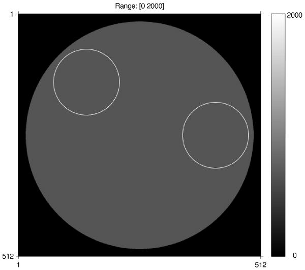
Ring phantom used for simulation study

Fig. 3.

Regularization penalty coefficients used in reconstruction of ring phantom. The four images are $r_{\mathit{\text{l}}}^j$ for l = 1, …, 4

We reconstructed images x̂ using several methods. We first created an image uniformly blurred by the target PSF. We then reconstructed images using (i) conventional regularization, r^j = 1, (m_l, n_l) = (0, 1), (1, 0), (ii) certainty based regularization [3], (iii) AIMA method with α = 0.1, (iv) AIMA method with α = 0, and (v) FIIN method with α = 0. Fig. 4 is a closeup of the right-most ring reconstructed with the various methods listed above and Fig. 5 is a closeup of the left-most ring.

Fig. 4.

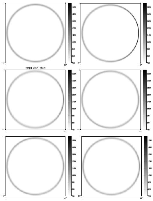
Images of right-most ring, Upper-Left: uniformly blurred by target PSF. Upper-Right: reconstructed using conventional regularization. Mid-Left: reconstructed using certainty-based regularization. Mid-Right: reconstructed using AIMA regularization, with α = 0.1. Lower-Left: reconstructed using AIMA regularization, with α = 0. Lower-Right: reconstructed using FIIN regularization, with α = 0.

Fig. 5.

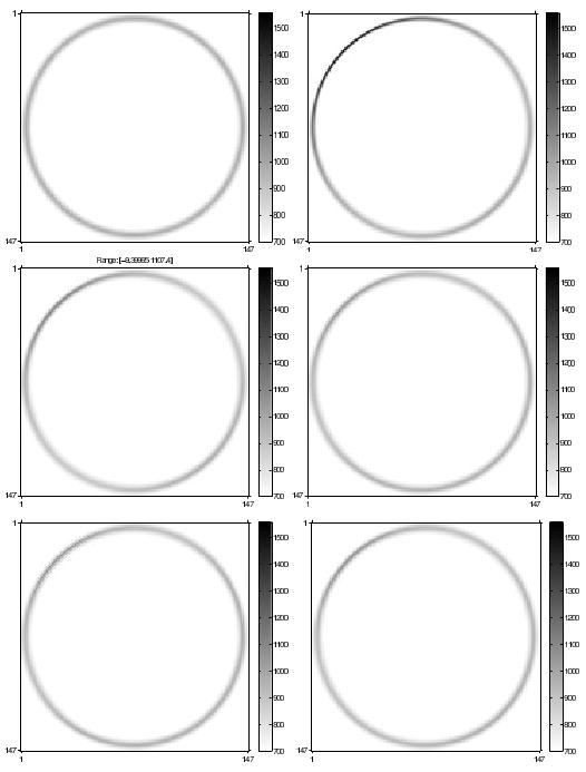
Images of left-most ring, Upper-Left: uniformly blurred by target PSF. Upper-Right: reconstructed using conventional regularization. Mid-Left: reconstructed using certainty-based regularization. Mid-Right: reconstructed using AIMA regularization, with α = 0.1. Lower-Left: reconstructed using AIMA regularization, with α = 0. Lower-Right: reconstructed using FIIN regularization, with α = 0.

Fig. 6 and Fig. 7 show profiles around the two rings of the reconstructed images using the various regularization methods relative to the mean intensity of the rings from our target, PULS reconstruction with conventional regularization. This verifies that AIMA and FIIN improve resolution uniformity. Here, 0 radians corresponds to the rightmost point of that ring and the angles are measured clockwise.

Fig. 6.

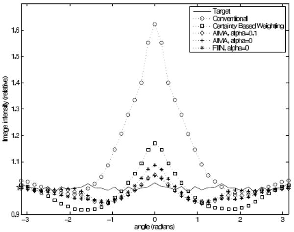
Profiles through the right-most ring from each reconstructed image.

Fig. 7.

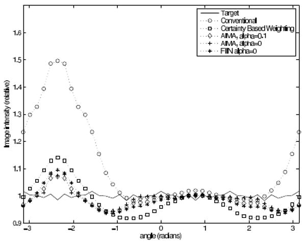
Profiles through the left-most ring from each reconstructed image.

The second study used a similar imaging geometry using one slice of real CT data from a GE scanner described in [18] with weightings W computed in the same way as [19]. ζ was selected such that the target PSF had a FWHM of 1.51 mm.

Fig. 8 displays an image reconstructed by PWLS using conventional regularization. The impulse response locations are denoted with crosses and a region is marked which will be displayed in Fig. 9. Fig. 9 show windowed reconstructions using conventional regularization, certainty based regularization, AIMA with α = 0.1 and α = 0, and FIIN with α = 0.

Fig. 8.

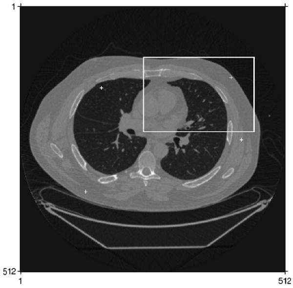
Reconstruction with conventional regularization without windowing with impulse responses marked

Fig. 9.

Reconstructions windowed from 800 to 1200 HUs using, from top to bottom, conventional regularization, certainty based regularization, AIMA with α = 0.1, AIMA with α = 0, FIIN with α = 0.

Fig. 10-13 show local impulse responses for the five regularization methods at several locations calculated analytically using (5). These figures show from left to right, the target impulse response, and local impulses responses for conventional regularization, certainty based regularization [3], AIMA with α = 0.1, AIMA with α = 0, and FIIN with α = 0. Contour plots of the LIR are displayed below at 0.9, 0.75, 0.5, 0.25, and 0.1 of the maximum value of the target PSF. The LIR becomes more anisotropic near the edge of the FOV. Our Fourier-based regularization scheme compensates for this anisotropy better than the certainty-based approach of [3].

Fig. 10.

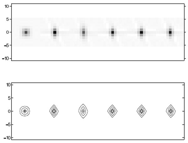
Impulse Responses at (-100,-100). From left to right, target, conventional regularization, certainty based regularization, AIMA regularization with α = 0.1, AIMA regularization with α = 0, FIIN regularization with α = 0.

Fig. 13.

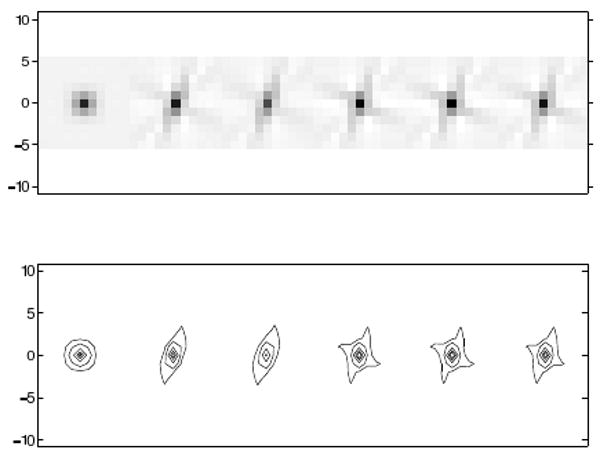
Impulse Responses at (-130,100). From left to right, target, conventional regularization, certainty based regularization, AIMA regularization with α = 0.1, AIMA regularization with α = 0, FIIN regularization with α = 0.

To quantify the performance of these regularizers on real CT data, we computed the PSF of the regularizers at every 10 pixels within the body. Then we calculated the FWHM of the PSFs at 181 evenly spaced angles, and computed the RMS error between the actual FWHM and the FWHM of the target. Histograms of these errors are displayed in Fig. 14. The mean of the RMS errors for conventional regularization, certainty based regularization, the AIMA method with α = 0.1, the AIMA method with α = 0, and the FIIN method with α = 0 are 2.7, 2.7, 2.3, 2.5, and 2.0 respectively.

Fig. 14.

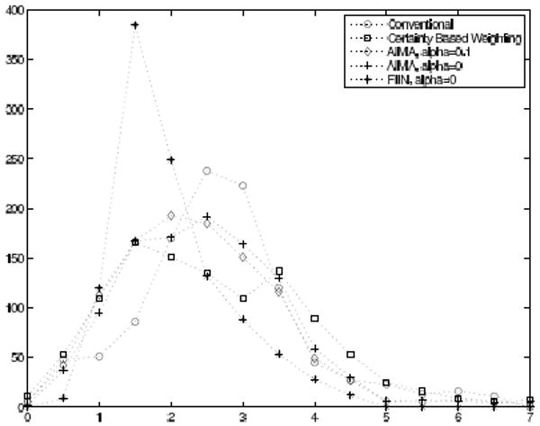
Plots of the error histogram for different impulse responses.

VI. Discussion

A. Spatial Resolution Properties

Fig. 4 and Fig. 5 provide a qualitative understanding of the spatial resolution properties of various regularization methods for the ring phantom. The phantom used consists of rings of uniform intensity and uniform width, thus images with uniform spatial resolution should have rings with uniform width and uniform intensity. Conventional regularization creates rings with sharper spatial resolution near the edge of the field of view. Certainty based regularization improves ring uniformity but anisotropy remains. The last three reconstructions using AIMA with α = 0.1, AIMA with α = 0 and FIIN provide rings that look almost identical, and which have a more uniform ring width than conventional, and certainty based regularization.

Fig. 6 and Fig. 7 show the amplitude of the rings traced clockwise. This confirms our initial assessment, that certainty based regularization achieves more uniform spatial resolution than conventional regularization, and that the AIMA and FIIN methods are all very similar and outperform the previous approaches.

Fig. 9 display a quadrant of windowed reconstructions using real CT data to illustrate the images produced using these regularization design methodologies. However, since we do not know the “truth” for this data, these images provide only a qualitative illustration of the effect of regularization design on spatial resolution. The impulse responses in Fig. 10-Fig. 13 illustrate the effect of regularization design on spatial resolution at various locations. These figures confirm that AIMA and FIIN methods improved isotropy over conventional and certainty-based regularization. The histogram plot of Fig. 14 and the mean of the PSF errors mentioned previously confirm this. AIMA has lower FWHM RMS error both certainty based regularization and conventional regularization. FIIN has the lowest FWHM RMS error, however it is much slower than AIMA.

The resulting impulse responses from the AIMA and FIIN methods are not completely isotropic. This may seem to contradict the dramatic improvement these regularization design methods achieved with the ring phantom. However, recall that we are trying to approximate w̃^j(Φ) using 3 basis functions (see §IV-A) for the AIMA, and 4 basis functions (see §A) for FIIN. With real data, w̃^j(Φ) is a complicated function that cannot be parameterized using 3 or 4 basis functions. This aspect, along with the non-negativity constraint limits the performance of any regularization design technique with a finite number of parameters. w̃^j(Φ) is much simpler for simple phantoms like the ring phantom, so AIMA yields better results there. Extensions of this regularization design to higher order penalties have the potential for more basis functions, and better performance.

The analysis of this paper focuses on the resolution nonuniformities cased by statistical weightings, not the resolution variation due to detector response and magnification. A more general regularization design with similar parameterization is discussed in [6]. Using the techniques in this paper to account for these effects is an open problem.

B. Computation Time

AIMA is quite efficient. Computing certainty based regularization takes the time of about 1 backprojection. In AIMA, we must first compute w̃^j(Φ) which takes the time of about 1 backprojection, and then solve the analytical solution which is very fast. FIIN also requires 1 backprojection to compute w̃^j(Φ), however it then has to run a non-negative least squares problem for every pixel. Though this is a fairly small NNLS problem, T is 4 × 4, it adds much compute time since it must be calculated for each pixel. In general, due to the faster compute times, we recommend AIMA with α = 0.1. If accuracy is more important than compute time, FIIN can be used instead.

VII. Conclusion and Future Work

The results presented indicate that we have a functional and efficient regularization design structure that yields approximately uniform and isotropic spatial resolution for 2D fan-beam systems. The methods also apply to the simpler case of 2D (parallel-beam) PET as described in [10]. In the future, we will extend these methods to 3D PET [9] and cone-beam CT. We will also study the noise properties. Another open question is how to design non-quadratic regularization [20].

Fig. 11.

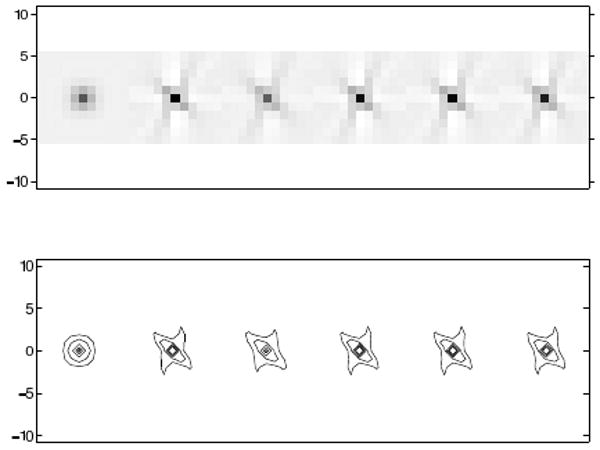
Impulse Responses at (150,-120). From left to right, target, conventional regularization, certainty based regularization, AIMA regularization with α = 0.1, AIMA regularization with α = 0, FIIN regularization with α = 0.

Fig. 12.

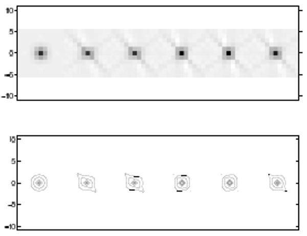
Impulse Responses at (170,0). From left to right, target, conventional regularization, certainty based regularization, AIMA regularization with α = 0.1, AIMA regularization with α = 0, FIIN regularization with α = 0.

Appendix A: Slower Regularization Design

This appendix describes the slower Double Integral Iterative NNLS, FIIN, method that does not use the AIMA approximation 2 − 2 cos(x) ≈ x² in (17) in the expression of the local frequency response of R. This design method is appropriately named because it uses the full integral over all frequency domain polar coordinates instead of just the angular coordinates. The matrices involved in this method are slightly more complex than those in AIMA so an iterative technique is needed. Converting (16) in §III-C into polar coordinates and combining with (15) yields

$$R^{\mathit{\text{j}}}(\rho ,\Phi )=\sum _{l=1}^L\frac{r_{\mathit{\text{l}}}^j}{n_l^2+m_l^2}(2-2cos(u_{\mathit{\text{l}}}(\rho ,\Phi ))),$$

where u_l(ρ, Φ) = n_l2πΔ_xρ cos(Φ) +m_l2πΔ_yρ sin(Φ). The target we use in regularization is the LIR associated with PULS at the center of the image, expressed in (23).

Following (25), we try to match the LIR at each pixel j to the target:

$$\begin{array}{l}\frac{w^j(\Phi )}{w^j(\Phi )+\beta \left|\rho \right|R^j(\rho ,\Phi )}\approx \frac{1}{1+\beta \left|\rho \right|0.5J(0)R_0(\rho ,\Phi )}\hfill \\ w^j(\Phi )+\beta \left|\rho \right|R^j(\rho ,\Phi )\approx w^j(\Phi )(1+\beta \left|\rho \right|0.5J(0)R_0(\rho ,\Phi ))\hfill \\ \beta \left|\rho \right|R^j(\rho ,\Phi )\approx \beta \left|\rho \right|0.5J(0)w^j(\Phi )R_0(\rho ,\Phi ))\hfill \\ R^j(\rho ,\Phi )\approx {\stackrel{\sim }{w}}^j(\Phi )R_0(\rho ,\Phi )),\hfill \end{array}$$

where w̃^j(Φ) = 0.5J(0)w^j(Φ). To design R, we use a method similar to that of §IV-A and project w̃^j(Φ)R₀(ρ, Φ)) onto the space spanned by {1 − cos(u_l(ρ, Φ))} that can be orthonormalized into L basis functions, {p_l(ρ, Φ)} using Gramm-Schmidt. Then our regularization design problem simplifies to

$${\text{r}}^j=\underset{\mathit{r}\ge 0}{\text{arg}min}{\Vert \mathit{\text{Tr}}-{\mathit{\text{b}}}^j\Vert }^2,$$ (32)

where b^j is a vector of inner products between w̃^j(Φ)R₀(ρ, Φ)) and the L orthonormal basis functions {p_l(ρ, Φ)}, $b_{\mathit{\text{k}}}^j=\int \int p_{\mathit{\text{k}}}(\rho ,\Phi ){\stackrel{\sim }{w}}^j(\Phi )R_0(\rho ,\Phi )d\mathit{\rho }d\Phi$, and T is a L × L matrix whose elements are the inner products between 2 − 2 cos(u_l(ρ, Φ)) and {p_l(ρ, Φ)}, T_mn = ∫ ∫ 2 − 2cos(u_m(ρ, Φ))p_n(ρ, Φ)dρdΦ. We define P to be an operator whose columns are {p₁, p₂, …p_L} so R(ρ, Φ) = PTr^j. This design problem is then solved with an NNLS algorithm. This more accurate version is slower than that presented in §IV-A because there is no apparent analytical solution similar to the one presented in §IV-C.

Appendix B: Analysis of Grammian Operator

This appendix considers fan-beam geometries and uses continuous-space analysis to analyze the Fourier transform of the Grammian operator A′W A to simplify the regularization design problem in (12). One can use polar coordinates Φ, ρ, and continuous-space analysis to separate the angular and radial components of A′W A. Using this framework, isotropy can be thought of as eliminating dependence on the angular component Φ.

A. Fan-Beam Geometry

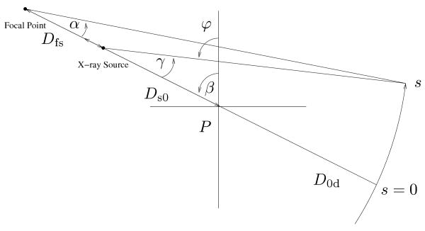
Fig. 15 illustrates the fan-beam geometry that we consider. Let P be the rotation isocenter. D_0d denotes the distance from the point P to the detector, D_s0 denotes the distance from the X-ray source to P, and D_fs denotes the distance from the X-ray source to the focal point of the detector arc. Define D_sd ≜ D_0d + D_s0 to be the total distance from the X-ray source to the center of the detector, and D_fd ≜ D_sd + D_fs to be the total distance from the focal point to the center of the detector. This formulation encompasses a variety of system configurations by allowing the detector focal point to differ from the X-ray source location. For flat detectors, D_fs = ∞. For third-generation X-ray CT systems, D_fs = 0. For fourth generation X-ray CT systems, D_fs = −D_s0.

Fig. 15.

Illustration of fan beam geometry.

Let s ∈ [−s_max, s_max] denote the (signed) arc length along the detector, where s = 0 corresponds to the detector center. Assuming detector elements are equally spaced along the detector, arc length is the natural parameterization. The various angles have the following relationships:

$$\begin{array}{l}\alpha (s)=\frac{s}{D_{\text{fd}}}\\ \gamma (s)={tan}^{-1}\left(\frac{\left(D_{\text{fd}}\right)sin\alpha (s)}{\left(D_{\text{fd}}\right)cos\alpha (s)-D_{\text{fs}}}\right)\end{array}$$

where the two most important cases are

$$\gamma (s)=\{\begin{array}{ll}\alpha (s),\hfill & D_{fs}=0\hfill \\ {tan}^{-1}s/D_{sd},\hfill & D_{fs}=\infty .\hfill \end{array}$$ (33)

The relationship between s and γ is:

$$s=\{\begin{array}{l}(D_{\text{fd}})\left[\gamma -arcsin\left(\frac{D_{\text{fs}}}{D_{\text{fd}}}sin\gamma \right)\right],\hfill \\ D_{\text{sd}}tan\gamma ,D_{\text{fs}}=\infty .\hfill \end{array}0\le D_{\text{fs}}<\infty$$ (34)

The ray corresponding to detector element s and angle β is (s, β) = {(x, y) : x cos φ(s, β) + y sin φ(s, β) = r(s)}, where

$$\begin{array}{c}\varphi (s,\beta )\triangleq \beta +\gamma (s)\hfill \\ r(s)\triangleq D_{\text{s}0}sin\gamma (s).\hfill \end{array}$$ (35)

The range of r depends on the position of the X-ray source and the size of the detector:

$$\left|r(s)\right|\le r_{max}\triangleq D_{\text{s}0}sin{\gamma }_{max},$$ (36)

where γ_max ≜ γ(s_max) and s_max is half the total detector arc length. The radius r_max defines the circular field of view of the imaging system. The fan angle is 2 γ_max.

The line-integral projection p(s, β) of f along (s, β) is²:

$$\begin{array}{ll}p(s,\beta )\hfill & ={\int }_{ℒ(s,\beta )}f(x,y)\text{d}\ell \hfill \\ \hfill & =\iint f(x,y)\delta (xcos(\varphi (s,\beta ))+ysin\varphi (s,\beta )-r(s))\text{d}x\text{d}y,\hfill \end{array}$$ (37)

for |s| ≤ s_max and 0 ≤ β < β_max. We require β_max ≥ π+2 γ_max to ensure complete sampling of the FOV (otherwise the impulse response would be highly anisotropic).

The usual inner product for fan-beam projection space is

$$\langle p_1,p_2\rangle ={\int }_{-s_{max}}^{s_{max}}{\int }_0^{{\beta }_{max}}{p}_1\left(s,\beta \right)p_2\left(s,\beta \right)\text{d}s\text{d}\beta .$$

Using this inner product in projection space, and the usual ² inner product in image space, the adjoint of is given by

$$\begin{array}{l}(\mathcal{P}\ast p)(x,y)={\int }_{-s_{max}}^{s_{max}}{\int }_0^{{\beta }_{max}}p\left(s,\beta \right)\hfill \\ \delta (xcos\varphi \left(s,\beta \right)+ysin\varphi \left(s,\beta \right)-r(s))p(s,\beta )\text{d}s\text{d}\beta ,\hfill \end{array}$$ (38)

where r(s) and φ(s, β) were defined in (35). We will next extend a common derivation of backproject then filter (BPF) tomographic reconstruction to accommodate a user defined weighting, and then change the coordinates from parallel-beam to fan-beam space.

B. Parallel-Beam Grammian Analysis

When we analyze the local impulse response, we typically consider recentered local impulse functions. In this derivation we will start with an uncentered local impulse response, and center it at the end by removing a phase term in the frequency domain. The un-centered local impulse response of the Grammian operator is,

$$\mathcal{\text{P}}\ast \mathcal{\text{WP}}{\mathit{\delta }}^j\left(x,y\right)={\int }_0^{\pi }{\int }_{-\infty }^{\infty }\delta (x^{j}cos(\phi )+y^{j}sin(\phi )-r)w(r,\phi )\delta (xcos(\phi )+ysin(\phi )-r)\mathit{\text{drd}}\phi .$$

Using the sampling property with the first δ, define

$$w^j(\phi )\triangleq w(r,\phi )=w(x^{j}cos(\phi )+y^{j}sin(\phi ),\phi ).$$ (39)

We denote the Fourier transform of δ^j(x, y) as F^j(ρ, Φ). Then, using the Fourier slice theorem,

$$\begin{array}{ll}\mathcal{P}\ast \mathcal{\text{WP}}{\mathit{\delta }}^j(x,y)\hfill & ={\int }_0^{\pi }{\int }_{-\infty }^{\infty }{\int }_{-\infty }^{\infty }{F}^j(\rho ,\phi )e^{\mathit{\text{i}}2\pi \rho r}d\rho w^j(\phi )\delta (xcos\phi +ysin\phi -r)\mathit{\text{drd}}\phi \hfill \\ \hfill & ={\int }_0^{\pi }{\int }_{-\infty }^{\infty }{F}^j(\rho ,\Phi )w^j(\phi )e^{\mathit{\text{i}}2\pi \rho (xcos\phi +ysin\phi )}d\rho d\phi .\hfill \end{array}$$ (40)

This is nearly the inverse Fourier transform in signed polar coordinates except for a ρ scale factor. Dividing by ρ,

$$\mathcal{P}\ast \mathcal{\text{WP}}{\mathit{\delta }}^j(x,y)={\int }_0^{\pi }{\int }_{-\infty }^{\infty }\frac{w^j(\phi )F({\delta }^j(x,y))}{\rho }{e}^{\mathit{\text{i}}2\pi \rho (xcos\phi +ysin\phi )}d\rho d\phi .$$

The local impulse response is recentered, h^j(x, y) = *δ^j(x+x^j, y+y^j) which eliminates the complex phase term F^j(ρ, φ). Then, the local frequency response is

$$H^j\left(\rho ,\Phi \right)=\frac{w^j(\Phi )}{\rho }.$$ (41)

C. Fan Beam Grammian Analysis

The natural indexing for fan-beam data is arc-length s and angle β. The analogs to r, ϕ for parallel-beam systems are r(s), ϕ(s, β) as defined in (35). The weighting expression w(r, ϕ) is indexed as w(s, β) in fan-beam coordinates. We start by looking at the fan-beam projection in terms of the analogs to parallel-beam coordinates,

$$\left(\mathcal{P}\ast \mathcal{\text{WP}}{\mathit{\delta }}^j\right)\left(x,y\right)={\int }_{-{\beta }_{max}}^{{\beta }_{max}}{\int }_{-s_{max}}^{s_{max}}w\left(s,\beta \right)\delta (x^{j}cos(\varphi (s,\beta ))+y^{j}sin(\varphi (s,\beta ))-r(s))\delta (xcos(\varphi (s,\beta ))+ysin(\varphi (s,\beta ))-r(s))\mathit{\text{dsd}}\beta .$$

We use the change of variables

$$r\prime =r(s)=D_{\text{s}0}sin\gamma (s)$$ (42)

$$\varphi \prime =\varphi (s,\beta )=\beta +\gamma (s)$$ (43)

as defined in (35) which has the corresponding Jacobian determinant

$$J(s)=\left|D_{\text{s}0}cos\gamma (s)\left|\right|\dot{\gamma }(s)\right|.$$ (44)

Then,

$$\begin{array}{l}(\mathcal{P}\ast \mathcal{\text{WP}}{\mathit{\delta }}^j)(x,y)={\int }_0^{2\pi }{\int }_{-r_{max}}^{r_{max}}w(r\prime ,\varphi \prime )\delta (x^{\mathit{\text{j}}}cos\varphi \prime +y^{\mathit{\text{j}}}sin\varphi \prime -r\prime )\delta (xcos\varphi \prime +ysin\varphi \prime -r\prime )\frac{1}{J(s(r\prime ))}\mathit{\text{drd}}\varphi .\end{array}$$

In this expression,

$$\begin{array}{c}w(r,\varphi )\triangleq w(s(r),\beta (r,\varphi ))\hfill \\ s(r)={\gamma }^{-1}(arcsin(r/D_{\text{s}0}))\hfill \\ \beta (r,\varphi )=\varphi -arcsin(r/D_{\text{s}0}).\hfill \end{array}$$

Using the sampling property of the first δ as in the parallel beam case,

$$w^j(\varphi \prime )\triangleq w(x^{j}cos\varphi \prime +y^{j}sin\varphi \prime ,\varphi \prime )$$ (45)

$$s^j(\varphi \prime )\triangleq s(r\prime ){\mid }_{r\prime =x^{j}cos\varphi \prime +y^{j}sin\varphi \prime }.$$ (46)

Again, let F^j(ρ, Φ) denote the Fourier transform of δ^j(x, y). Then, using the Fourier slice theorem,

$$\begin{array}{l}(\mathcal{P}\ast \mathcal{\text{WP}}{\mathit{\delta }}^j)(x,y)\\ ={\int }_{-r_{max}}^{r_{max}}{\int }_0^{2\pi }{\int }_{-\infty }^{\infty }\frac{F^j(\rho ,\Phi )w^j(\varphi \prime )}{J(s^j(\varphi \prime ))}{e}^{\mathit{\text{i}}2\pi pr\prime }\delta (xcos\varphi \prime +ysin\varphi \prime -r\prime )d\rho d\varphi \prime dr\prime \\ ={\int }_0^{2\pi }{\int }_{-\infty }^{\infty }\frac{F^j(\rho ,\Phi )w^j(\varphi )}{J(s^j(\varphi \prime ))}{e}^{\mathit{\text{i}}2\pi \rho (xcos\varphi \prime +ysin\varphi \prime )}d\rho d\varphi \prime \\ ={\int }_0^{\pi }{\int }_{-\infty }^{\infty }\frac{F^j(\rho ,\Phi )w^j(\varphi \prime )}{J(s^j(\varphi \prime ))}{e}^{\mathit{\text{i}}2\pi \rho (xcos\varphi \prime +ysin\varphi \prime )}d\rho d\varphi \prime \\ +{\int }_0^{\pi }{\int }_{-\infty }^{\infty }\frac{F^j(\rho ,\Phi )w^j(\varphi ″)}{J(s^j(\varphi ″))}{e}^{\mathit{\text{i}}2\pi \rho (xcos\varphi ″+ysin\varphi ″)}d\rho d\varphi ″,\end{array}$$

where φ″ = φ′ + π. This is similar to the parallel-beam derivation except that we have two integrals. We can convert each integral into the inverse Fourier transform as we did in the parallel-beam case and strip out the phase term F^j(ρ, Φ) by recentering the local impulse response. The local frequency responses of the Grammian operator is

$$H^j(\rho ,\Phi )=\frac{{\stackrel{\sim }{w}}^j(\Phi )}{\left|\rho \right|},$$ (47)

where,

$${\stackrel{\sim }{w}}^j(\Phi )=\frac{1}{J(s^j(\Phi ))}\left[w^j(\varphi ){|}_{\varphi =\Phi }+w^j(\varphi ){|}_{\varphi =\Phi +\pi }\right].$$ (48)

Because of the absolute value function in (44), J(s) is invariant to the π phase shift. For the case where we have uniform weighting, w(s, β) = 1 and therefore W = I, and (47) simplifies to

$$H^j(\rho ,\Phi )=\frac{2}{J(s^j(\Phi ))\left|\rho \right|}.$$ (49)

We use this equation in the calculation of a target local impulse response (24).

Appendix C: Derivations of the analytical solution

In this appendix, we show that $\sqrt{d_2^2+d_3^2}\le d_1$, as claimed below (31) in §IV-C. Squaring the integrals in (31), we have:

$$\begin{array}{l}{d}_1^2=\frac{1}{\pi }{\int }_0^{\pi }{\int }_0^{\pi }{w}^{\mathit{\text{j}}}(X)w^{\mathit{\text{j}}}(Y)\mathit{\text{dX dY}}\\ d_2^2=\frac{1}{\pi }{\int }_0^{\pi }{\int }_0^{\pi }cos(2X)w^{\mathit{\text{j}}}(X)cos(2Y)w^{\mathit{\text{j}}}(Y)\mathit{\text{dX dY}}\\ d_3^2=\frac{1}{\pi }{\int }_0^{\pi }{\int }_0^{\pi }sin(2X)w^{\mathit{\text{j}}}(X)sin(2Y)w^{\mathit{\text{j}}}(Y)\mathit{\text{dX dY}}.\end{array}$$

In particular,

$$\begin{array}{ll}{d}_2^2+d_3^2\hfill & =\frac{1}{\pi }{\int }_0^{\pi }{\int }_0^{\pi }{w}^{\mathit{\text{j}}}(X)w^{\mathit{\text{j}}}(Y)\left[cos(2X)cos(2Y)+sin(2X)sin(2Y)\right]\mathit{\text{dX dY}}\hfill \\ \hfill & =\frac{1}{\pi }{\int }_0^{\pi }{\int }_0^{\pi }{w}^{\mathit{\text{j}}}(X)w^{\mathit{\text{j}}}(Y)cos(2X-2Y)\mathit{\text{dX dY}}.\hfill \end{array}$$

Thus, $d_2^2+d_3^2\le d_1^2$ since w^j(Φ) ≥ 0 for all Φ and cos(2X − 2Y) ≤ 1 for all X and Y.

References

- 1.Fessler JA. Statistical image reconstruction methods for transmission tomography. In: Sonka M, Fitzpatrick J Michael, editors. Handbook of Medical Imaging, Volume 2. Medical Image Processing and Analysis. SPIE; Bellingham: 2000. pp. 1–70. [Google Scholar]
- 2.Fessler JA. Penalized weighted least-squares image reconstruction for positron emission tomography. IEEE Trans Med Imag. 1994 Jun;13(2):290–300. doi: 10.1109/42.293921. [DOI] [PubMed] [Google Scholar]
- 3.Fessler JA, Rogers WL. Spatial resolution properties of penalized-likelihood image reconstruction methods: Space-invariant tomographs. IEEE Trans Im Proc. 1996 Sep;5(9):1346–58. doi: 10.1109/83.535846. [DOI] [PubMed] [Google Scholar]
- 4.Joseph PM. The influence of modulation transfer function shape on CT image quality. Radiology. 1982 Oct;145(1):179–85. doi: 10.1148/radiology.145.1.7122876. [DOI] [PubMed] [Google Scholar]
- 5.Stayman JW, Fessler JA. Regularization for uniform spatial resolution properties in penalized-likelihood image reconstruction. IEEE Trans Med Imag. 2000 Jun;19(6):601–15. doi: 10.1109/42.870666. [DOI] [PubMed] [Google Scholar]
- 6.Stayman JW, Fessler JA. Compensation for nonuniform resolution using penalized-likelihood reconstruction in space-variant imaging systems. IEEE Trans Med Imag. 2004 Mar;23(3):269–84. doi: 10.1109/TMI.2003.823063. [DOI] [PubMed] [Google Scholar]
- 7.Nuyts J, Fessler JA. A penalized-likelihood image reconstruction method for emission tomography, compared to post-smoothed maximum-likelihood with matched spatial resolution. IEEE Trans Med Imag. 2003 Sep;22(9):1042–52. doi: 10.1109/TMI.2003.816960. [DOI] [PubMed] [Google Scholar]
- 8.Qi J, Leahy RM. Resolution and noise properties of MAP reconstruction for fully 3D PET. IEEE Trans Med Imag. 2000 May;19(5):493–506. doi: 10.1109/42.870259. [DOI] [PubMed] [Google Scholar]
- 9.Shi H, Fessler JA. Quadratic regularization design for 3d cylindrical PET. Proc IEEE Nuc Sci Symp Med Im Conf. 2005;4:2301–5. [Google Scholar]
- 10.Fessler JA. Analytical approach to regularization design for isotropic spatial resolution. Proc IEEE Nuc Sci Symp Med Im Conf. 2003;3:2022–6. [Google Scholar]
- 11.Shi H, Fessler JA. Quadratic regularization design for fan beam transmission tomography. Proc SPIE 5747, Medical Imaging 2005: Image Proc. 2005:2023–33. [Google Scholar]
- 12.Fessler JA. Technical Report 297. Comm and Sign Proc Lab, Dept of EECS, Univ of Michigan; Ann Arbor, MI: Aug, 1995. Resolution properties of regularized image reconstruction methods; pp. 48109–2122. [Google Scholar]
- 13.Li Q, Asma E, Qi J, Bading JR, Leahy RM. Accurate estimation of the Fisher information matrix for the PET image reconstruction problem. IEEE Trans Med Imag. 2004 Sep;23(9):1057–64. doi: 10.1109/TMI.2004.833202. [DOI] [PubMed] [Google Scholar]
- 14.Clinthorne NH, Pan TS, Chiao PC, Rogers WL, Stamos JA. Preconditioning methods for improved convergence rates in iterative reconstructions. IEEE Trans Med Imag. 1993 Mar;12(1):78–83. doi: 10.1109/42.222670. [DOI] [PubMed] [Google Scholar]
- 15.Lawson CL, Hanson RJ. Solving least squares problems. Prentice-Hall; 1974. [Google Scholar]
- 16.Fessler JA. Matlab tomography toolbox. 2004. Available from http://www.eecs.umich.edu/∼fessler.
- 17.De Man B, Basu S. Distance-driven projection and backprojection. Proc IEEE Nuc Sci Symp Med Im Conf. 2002;3:1477–80. [Google Scholar]
- 18.Thibault JB, Sauer K, Bouman C, Hsieh J. A three-dimensional statistical approach to improved image quality for multi-slice helical CT. Med Phys. 2007 Nov;34(11):4526–44. doi: 10.1118/1.2789499. [DOI] [PubMed] [Google Scholar]
- 19.Thibault JB, Bouman CA, Sauer KD, Hsieh J. A recursive filter for noise reduction in statistical iterative tomographic imaging. Proc SPIE 6065, Computational Imaging IV. 2006:60650X. [Google Scholar]
- 20.Ahn S, Leahy RM. Spatial resolution properties of nonquadratically regularized image reconstruction for PET. Proc IEEE Intl Symp Biomed Imag. 2006:287–90. [Google Scholar]