Automatic Classification of Lymphoma Images with Transform-Based Global Features

Abstract

We propose a report on automatic classification of three common types of malignant lymphoma: Chronic Lymphocytic Leukemia, Follicular Lymphoma, and Mantle Cell Lymphoma. The goal was to find patterns indicative of lymphoma malignancies and allowing classifying these malignancies by type. We used a computer vision approach for quantitative characterization of image content. A unique two-stage approach was employed in this study. At the outer level, raw pixels were transformed with a set of transforms into spectral planes. Simple (Fourier, Chebyshev, and wavelets) and compound transforms (Chebyshev of Fourier and wavelets of Fourier) were computed. Raw pixels and spectral planes then were routed to the second stage (the inner level). At the inner level, the set of multi-purpose global features was computed on each spectral plane by the same feature bank. All computed features were fused into a single feature vector. The specimens were stained with hematoxylin (H) and eosin (E) stains. Several color spaces were used: RGB, gray, Lab, and also the specific stain-attributed H&E space, and experiments on image classification were carried out for these sets. The best signal (98-99% on previously unseen images) was found for the HE, H, and E channels of the H&E data set.

I. Introduction

Tymphoma [1] is a clonal malignancy that develops in lymphocytes. Lymphoma [1] is a clonal malignancy that develops in lymphocytes. It can develop in either T- or Bcells though about 85% of cases are B-cell-derived. The WHO Classification of Lymphoid Malignancies includes at least 38 named entities. Lymphoma types are usually distinguished by their pattern of growth and the cytologic features of the abnormal cells. In addition, genetic, immunologic, and clinical features often aid in making the diagnosis. However, the most important diagnostic criteria for lymphoma are the morphologic features of the tumor as observed by light microscopy of hematoxylin- and eosinstained tissue sections and interpreted by an experienced hematopathologist. Lymphoid malignancies were diagnosed in nearly 115,000 people in 2008 [2].

Pathologists make a distinction between malignant and healthy (or benign) tissue, and further differentiate between malignancy types. These distinctions are essential because the diagnosis allows predictions of the natural history of disease and guides treatment decisions [3]. Typically pathologists identify a tumor by visual inspection of a mounted tissue sample on microscope slides using high and low magnifications. Searching for patterns in medical images could be facilitated by implementing recent breakthroughs in computer vision [4, 5].

Pattern classifiers are commonly implemented in content-based image analysis. However, several uncertainties pose significant challenges to achieving accurate classification of lymphoma. First, histological lymphoma features may not be present across the whole area of a slide. Second, it is unclear that a single magnification is capable of distinguishing the different types. Third, an individual tumor may contain a range of cell types that, while derived from the same clone, do not share cytologic features. Fourth, individual types of tumors may be heterogeneous. For example, follicular lymphoma contains at least two types of cells and the relative proportions of the two types are used to grade the tumor. Another type, mantle cell lymphoma, exhibits several patterns. A useful classifier should account for the range of histologies that comprise a single disease entity.

Computer vision methods [4-6] are emerging as a new tool in medical imaging [5, 7-9], bridging a gap between cancer diagnostics [3, 10] and pattern analysis. Nearly all cancer classification based on computer vision methods relies on identifying individual cells, requiring segmentation or pre-selected ROIs. The reliance on segmentation leads to the use of image features highly specific to cell biology, or in more extreme cases, only capable of processing H&E-stained cells or limited to specific stains and specific cell types. However, despite these limitations, segmentation has proven effective for the diagnosis of selected cancer types. In several studies, overall classification accuracy was as high as 90%, comparing favorably with pathologists, even exceeding the accuracy of human scorers in some cases.

In biology, biomedicine and related fields, an image processing approach without prior assumptions or constraints may be of considerable interest. Biomedical applications produce images of many kinds [4, 6] where there is neither a typical imaging problem, nor a typical set of content descriptors. This diversity of image types requires either a broad variety of application-specific algorithms, or an approach that is not application-specific. Avoiding task-specific preprocessing steps will lead to the development of more general machine vision approaches that could be applied to a greater number of imaging problems in biology and medicine.

The general method we developed (WND-CHARM, [11]) has been previously characterized in a diverse set of imaging problems. These included standard pattern recognition benchmarks such as face recognition, object and texture identification [11], and detection of comet dust tracks in aerogel [12]. Biological microscopy applications included identification of sub-cellular organelles [11, 12], classification of pollen [11, 12], characterization of physiological age and muscle degeneration in C. elegans [13, 14], and scoring of high-content imaging screens [12]. Human knee Xrays were also analyzed to diagnose osteoarthritis [15], predict osteoarthritis risk [16], as well as identify individuals from these radiographs [17]. Much of this work is summarized in an imaging benchmark for biological applications called IICBU-2008 [18]. All of these applications of WND-CHARM used the same set of algorithms with the same parameters, differing only in the arrangement of images into training classes. Several of these examples required discriminating morphologies in images of cellular fields, which are traditionally pre-processed using segmentation. Examples include high-content screens for absence of centromeres, presence of binucleate cells, and morphology of phylopodia [12, 18].

In this report, we present an experimental study of three common types of lymphoma (see in Fig. 1): chronic lymphocytic leukemia / small lymphocytic lymphoma (CLL), follicular lymphoma (FL), and mantle cell lymphoma (MCL). These are the three most common types of lymphoma, and were chosen because of their clinical relevance. The lymphoma cases used in this study were chosen to be representative of the three lymphoma classes, consisting of typical morphologies that could be used for training human pathologists. This slide collection contained significant variation in sectioning and staining and was thus more representative of slides commonly encountered in a clinical setting rather than being representative of the type more commonly found under tightly controlled laboratory conditions. The high degree of variation prompted us to compare the relative information content in grayscale, the original three RGB channels, a color transformation into CIE-L* a*b* (Lab) color space, and a reconstruction of the RGB channels into hematoxylin and eosin channels (HE). Furthermore, generic image features from these color spaces were analyzed using three different classifiers, including WND-CHARM’s weighted-neighbor distance (WND), radial basis functions (RBF) and a naïve Bayes network (BBN).

Fig. 1.

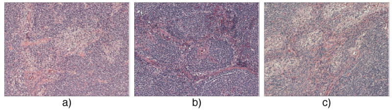
Patterns for three lymphoma types: a) CLL, pale areas as proliferation centers; b) FL, follicular structure; c) MCL, neoplastic lymphocytes in the diffuse/blastic sub-type.

Our findings were that the WND classifier operating on E channel of the HE color space produced an average classification rate of 99% for the three tissues. Significant differences in classification accuracies were found between the four color spaces tested, with HE consistently more accurate than the others followed by RGB, grayscale and Lab. The relative accuracies obtained in these color spaces were consistent between the three classifiers used. The differences in classification accuracies between the three classifiers were not as pronounced, with WND and RBF producing nearly the same accuracies for all four color spaces and slightly lower results for BBN. We also tested three feature selection algorithms for WND, including Fisher linear discriminant (FLD), minimum redundancy maximum relevance (mRMR), and a Fisher/Correlation algorithm (F/C) described below. As with the classifier comparisons, there were no significant differences between these three feature selection algorithms. The only significant differences in classification accuracy found in this study were attributed to the different representations of the color information in these images.

Our report is organized in the following way: Section II discusses image content and describes the features used; Section III discusses the relative contributions of morphological and color information. The classifiers employed are described in Section IV, and Section V reports results of classification. Section VI contains the discussion, followed by future work in Section VII, and a summary in Section VIII.

II. Content And Features

A. Summary of Previous Work

As mentioned in the introduction, much of the previous work in lymphoma classification and medical image processing of tissues in general involves a prior segmentation step to identify cells, nuclei, or other cellular structures. Important advances were made in this field using segmentation (summarized below and in Table I), and serve as a basis of comparison for our approach that does not rely on segmentation. In many cases, the initial segmentation step is used as a basis for extracting generic image features followed by classification algorithms, similarly to what we have done. Other than the lack of segmentation, our approach differs in the quantity of generic image descriptors generated, as well as the resulting need to adopt an automated dimensionality reduction technique.

TABLE I.

Source	Class Number	Segmentation	Accuracy Reported	Color
Sertel et al [7]	3	Yes	90.3%	Yes
Foran et al [11]	4	Yes	89%	Yes
Tuzel et al [9]	5	Yes	89%	No
Nielsen et al [8]	2	Yes	78%	No
Tabesh et al [5]	2	Yes	96.7%	Yes
Monaco et al [50]	2	Yes	79%	No
This work	3	No	99%	Yes

Comparison of reported results in the relevant research.

In [7] Sertel et al. used color texture analysis for classifying grades of malignant lymphoma (FL), achieving 90.3% accuracy. Foran et al. [19] applied elliptic Fourier descriptors and multi-resolution textures to discriminate between lymphoma malignancies. A total of four classes were used, including three lymphoma types and one normal tissue. This computational approach (89% accuracy) outperformed the traditional method of evaluation by expert pathologists (66%). In [9] the authors used machine vision to discriminate five lymphoma types. They used texton histograms as image features and applied a Leave One Out test strategy to obtain an overall classification accuracy of 89%. Notably, they reported 56% correct classification for their worst data type (FL). Nielsen et al. [8] studied ovarian cancer cells using adaptive texture feature vectors from class distance and class difference matrices. They reported 78% correct classification for a two class problem (good and bad prognosis). In [20] the authors applied the back-propagation neural network to diagnose pathology of lymph nodes. The two classes in the study were malignant nodes (metastasis of lung cancer) and benign tissue (sarcoidosis). Their computer vision approach resulted in higher classification accuracy (91%), than the diagnostic accuracy of a surgeon with five years of experience (78%). In [21] Monaco et al. used probabilistic Markov models for classifying prostate tissues; they reported overall classification accuracy 79% on a two-class problem.

B. Mapping Pixels to a Global Feature Space

It is inefficient to deal directly with pixels when learning patterns, which leads to the concept of mapping pixels into feature space [22], for applications like classification, search and retrieval [23, 24]. We note that there are some methods for texture analysis dealing directly with local pixel neighborhoods (see in [9]) or under-sampling the original images (as in [25]).

Let us define I = ℝ^m×n as the image pixel plane, and f⃗ as its corresponding ℝ^N×1 feature vector. Then the mapping ${ℝ}^{m\times n}\stackrel{\psi }{\to }{ℝ}^{N\times 1}$ can be expressed in the form f⃗ = ψ (I). This conversion could be performed with a function, equation, algorithm, or a combination of algorithms (the later was used in this study). The conversion does not require images to have the same dimensions, while the resulting feature space has the same dimensionality for all images.

The mapping implemented in this report is a composite of several algorithms. The feature set encompasses a representative collection of global features [11] assessing texture content, edges and shapes, coefficients in polynomial decompositions, and general statistics, as shown in Table II. The feature set contains eleven families of different algorithms for numerical assessment of the content. Experiments performed in [11, 12, 14, 18] convincingly support the assertion about efficacy of this feature set for diverse imaging applications.

TABLE II.

Feature Name	Output Size
Polynomial Section
Chebyshev features	32
Zernike features	72
Chebyshev-Fourier features	32
Texture Section
Tamura features	6
Haralick features	28
Gabor features	7
Other Features
Radon features	12
Multi-scale histograms	24
First four moments with comb filter	48
Edge statistics	28
Object statistics	34

Feature vector output sizes. The raw pixels and spectral planes (transforms) were fed into the feature bank in the computational chain.

C. Fusing Features: Two-Stage Approach

We used the two-stage approach suggested in [11]. In this method, the raw pixels at the outer level were transformed with a set of given transforms to corresponding spectral planes. The organization of the transforms is given in Fig. 2. The approach used Fourier (FFTW [26]), Chebyshev and wavelet (symlets5¹, level-1 details) transforms. The compound transforms producing super-spectral planes included Chebyshev of Fourier and wavelets of Fourier. The set of multi-purpose global features [11, 14] was computed for every pixel plane (transforms included) by the same feature bank (described in previous section). Finally, all computed features were fused into a single feature vector. Therefore, all algorithms for multi-purpose features (see also in Table II) – combined with several transforms – resulted in a vector of 1025 elements. We refer to the scheme shown in Fig. 2 as a computational chain.

Fig. 2.

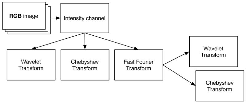
Use of transforms in the framework: three simple transforms (wavelets, Chebyshev and Fourier) and two compound transforms (Chebyshev of Fourier and wavelets of Fourier). The feature bank is applied to each pixel plane shown.

Using spectral features in pattern analysis is not entirely new [23, 24]; on the other hand, fusing features from different transforms for enhancing class discrimination is not common either. The motivation for this way of combining features came from the realization that mapping pixels into spectral planes is equivalent to using alternative content for the same classification problem. The given set of transforms is linear with respect to intensity but is non-linear with respect to pixel indices with the result that different spectral planes generate a variety of diverse patterns.

Therefore, the desire for a multi-purpose feature set that could be used across the entire biological or medical domain can, in fact, be fulfilled with a rather moderate set of basic features. Another advantage of using transforms is that there is little incremental cost for their development, but a multiplicative increase in feature diversity, with essentially all of the cost being computational. To some extent, the idea of fusing different spectral planes together is similar to the concept of multi-scale representation: it also allows assessing content from multiple perspectives. We will pursue this topic elsewhere.

D. Spectral Features and Their Meaning

Previous work on constructing global descriptor sets was reviewed in Gonzalez & Woods [24], with more recent work by Rodenacker & Bengtsson [4] and Gurevich & Koryabkina [27]. It should be noted that the authors manifest their feature sets as algorithm toolboxes, and they promote the idea of specialized feature sets for each particular imaging application. Such an approach suffers from the shortcoming that an expert opinion is needed to select the useful features for every new imaging problem. Further, minor changes in acquisition parameters could invalidate this expert-selected set of optimal descriptors. In contrast, in the approach suggested in [11] the global feature set is intended to be used as a whole, without manual selection of particular algorithms a priori. Instead, we automate the selection and weighting of these features for each imaging task.

In biomedical image processing, application-specific features tend to be more commonly used than generic global descriptors [6, 28, 29]. Indeed, there are clear advantages to using domain-specific features: they allow to work in smaller feature spaces, are faster to compute and often allow some parameter tuning for achieving higher accuracy. Unfortunately, specific features restrict expansion to different applications that can be a disadvantage in biology and biomedicine, where there are many image types in common use.

For certain classification problems, features have valuable scientific meaning, and often the selected subsets have a clear interpretation. A good example is the relative expression of genes used as features when classifying microarray experiments [30]. In contrast, in the transform-based feature set, the interpretation of even the most intuitive features (such as FFT-based descriptors) is rather more limited. In some studies of malignancy patterns (as in [5]) authors characterize the selected features as visual cues and consider them potentially useful. The generality of the feature set we employ precludes any guarantees that the selected or most highly ranked features will be visually informative or interpretable. However, it is possible that even in this general set, selected features can lead directly to interpretable visual cues [31]. Additionally, by classifying sub-regions of images, it is possible to identify where the classification signal is greatest, potentially leading to spatial visual cues [16].

E. Feature Ranking and Feature Selection

Fig. 3 outlines the general classification scheme. We employed the Fisher Linear Discriminant [23] (FLD) as our major feature ranking tool. In multi-class problems the FLD operates on ‘between’ and ‘within’ data variations as ${\overrightarrow{S}}_B={\sum }_c{N}_c{\parallel {\overrightarrow{\mu }}_c-\overline{\overrightarrow{\mu }}\parallel }_2^2,{\overrightarrow{S}}_W={\sum }_c{{\sum }_{j\in c}\parallel {\overrightarrow{X}}_j^{(c)}-{\overrightarrow{\mu }}_c\parallel }_2^2$, and the class separation score is the ratio ${\overrightarrow{w}}_{\mathrm{Fisher}}={\overrightarrow{S}}_B/{\overrightarrow{S}}_W$. Here ${\overrightarrow{X}}_j^{(c)}$ are the training samples in class c, μ⃗_c are class average, $\overline{\overrightarrow{\mu }}$ is the average on all classes, and N_c is the number of training samples in the c -th class.

Fig. 3.

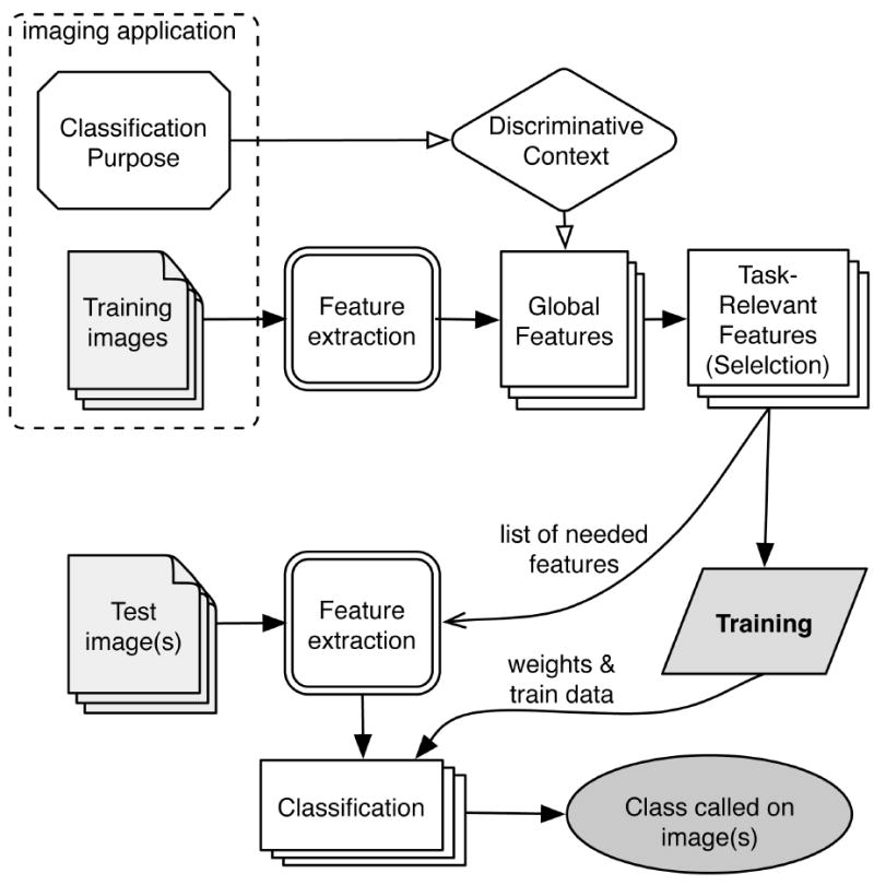
Multi-purpose features are computed and weighted in accordance to their task-specific discriminative power. Weighted features are used by the WND classifier.

Similarly to the Fisher score, the colinearity measure ranks each individual feature as a ratio of between/within data scattering with different figures measuring data variations. The colinearity approach operates in terms of angles between individual samples ${\mathbf{p}}_k,{\mathbf{p}}_l:{\alpha }_{\mathit{kl}}=\cos \left({\mathbf{p}}_k,{\mathbf{p}}_l\right)=\langle {\mathbf{p}}_k,{\mathbf{p}}_l\rangle /p_k{p}_l$. Let the vector f be an arbitrary row of data X, then $\mathbf{f}={\cup }_c{\mathbf{p}}_c$ is a combination of partitions belonging to different classes. The variation between different classes for this row can be measured with ${\alpha }^B=\underset{k,l}{\mathrm{mean}}{\alpha }_{k,l}$ for all C (C − 1)/2 pairs of k, l. Now, if ${\stackrel{⌢}{\mathbf{q}}}_s^c,{\stackrel{⌣}{\mathbf{q}}}_s^c$ are two randomly shuffled sub-samples of p_c, then the within-class variation is ${\alpha }^W=\underset{c,s}{\mathrm{mean}}\left\{\cos \left({\stackrel{⌢}{\mathbf{q}}}_s^c,{\stackrel{⌣}{\mathbf{q}}}_s^c\right)\right\}$. The corresponding feature score here is ${\overrightarrow{w}}_{\mathrm{Coll}}={\overrightarrow{\alpha }}_B/{\overrightarrow{\alpha }}_W$. The third ranking scheme used the Pearson correlation coefficient ${\overrightarrow{w}}_{\mathrm{Pears}}=\rho \left({\left\{X_{\mathit{fj}}\right\}}_{j=1}^{N_c},\overrightarrow{\zeta }\right)$ describing the correlation between the given feature and the intended class values ζ⃗ (as the ground truth).

FLD was implemented to select features having the most discriminative power. We gradually increased the pool of selected features by starting with the highest ranked features, progressing to less discriminative ones, and stopping feature addition once classifier performance stops improving. We also used a heuristic F/C approach for subspace construction:

For each candidate feature to be added to the feature pool, we compute a Pearson correlation between the candidate and each feature in the pool. The average of these correlations is the denominator in a ratio where the numerator is the candidate feature’s Fisher score. Features are added to the pool in descending order of their Fisher score until this ratio stops increasing. In this way, features are selected that have highest Fisher discrimination and least Pearson correlation at the same time. A third method for feature selection was the mRMR algorithm [32], which maximizes relevance (discrimination) while minimizing redundancy. Comparison of these three feature selection algorithms are shown in Table VI and discussed further in Section V.

TABLE VI.

Data Set	FLD	MRMR	F/C
Gray	0.85 ± 0.03	0.81 ± 0.03	0.85 ± 0.02
RGB	0.90 ± 0.02	0.87 ± 0.03	0.89 ± 0.01
Lab	0.74 ± 0.02	0.71 ± 0.02	0.73 ± 0.02
HE	0.98 ± 0.01	0.98 ± 0.01	0.98 ± 0.00

Comparison of different feature selection techniques (WND classifier used) on Gray, RGB, Lab, and HE data sets. Top classification accuracy values are in bold. All three methods report close results.

III. Lymphoma Data: Morphology And Color

A. Malignancy Patterns

Although there are as many as 38 different lymphoma types, the three most clinically significant B-cell derived lymphomas were selected for this study. These three major types are also commonly used in other machine-classification studies (see Table I).

Depending on the magnification, malignancy patterns in pathology specimens are revealed jointly by the texture and low-to-mid scale spatial features of the image. Specifically, the common pattern for the CLL type in low resolution shows pale areas (nodules) that are interpreted to be proliferation centers (Fig. 1). In high magnification, these areas show small cleaved cells (small round nuclei) with condensed chromatin that cause their relative paleness at lower magnification. Abundant pale cytoplasm at high resolution may also be indicative of CLL type [33].

The MCL malignancies in high resolution feature irregularly shaped nuclei; in low magnification MCL type may reveal several patterns, including mantle zone, nodular, diffuse, and blastic. In diffuse and blastic types (see in Fig. 1) neoplastic lymphocytes replace the node. Given high structural variability, the MCL type is often difficult to diagnose. For the FL type, low magnification exhibits the follicular pattern, with regularly shaped nuclei in higher magnifications.

B. Color as an Experiment Variable

From the pathologist’s standpoint, color has no direct involvement in diagnostics of the sample; malignancy of the tissue is reflected in morphology. At the same time, histopathology specimens are colored to highlight the morphology of nuclei and cytoplasm [10, 34, 35]. One of most commonly used stain combinations is Hematoxylin-Eosin (H&E), targeting nuclei and cytoplasm, respectively. It is not quite clear a priori whether the signal is in the nuclear and cytoplasmic morphology exclusively, or whether color itself also plays a role, for example due to the interaction of the two stains. As one can see from Table I, use of color in analyzing histopathology images is not uncommon. Approaches on color use in these applications range from mainstream techniques (color histograms [36] or color moments [37]) to color textures [38] and unusual solutions for color quantization, as in [7, 39]. The CIE-L*a*b (Lab) color space is often used for analysis of H&E-stained samples [40-42] and color images in general [43] due to its ability to represent color in a device-independent and perceptually uniform way.

An issue with H&E stain is that the relative intensity is subject to variation, case-to case and hospital-to-hospital. This stain variability, especially pronounced in the samples used in this study, led us to avoid the use color features. Instead, we treated color as an experimental variable. We used four separate color schemes to discern the three types of malignancy in our lymphoma set. The first scheme is a grayscale intensity computed from the RGB colors using the NTSC transform [44], where the intensity value is Gray = [0.2989 0.5870 0.1140 ] × [R G B]^T.

Second, we used a standard RGB color scheme which was the direct camera output. Third, Lab color scheme. This representation of colors implements perceptual uniformity of the luminance scale [44, 45]. Lab color is a nonlinear scaling of device-dependent RGB signals producing an orthogonal space where distances between colors correspond to perceived color differences [7, 39, 41, 46]. Our motivation for using Lab scheme was to minimize the within-class variation of stain color. Lastly, the fourth color scheme required color deconvolution, as described in the next sub-section.

C. Color Deconvolution

In H&E staining, hematoxylin targets cell nuclei (blue), and eosin stains the cytoplasm red. Combinations of stained nuclei and cytoplasm form macro patterns that are indicative of hematologic malignancies [10, 34, 35]. The color CCD camera collects a tri-color RGB image, while the original signal has only two components, representing chromatin and cytoplasm.

One important aspect is that dyes (H&E) have complex overlapping spectra. Ruifrock and Johnston [47] suggested a deconvolution method for the separation of overlapping spectra into independent channels corresponding to H&E stain concentrations in the specimen. The optical density is measured on representative areas having highest stain concentrations. The optical density of the dye (i.e., the pixel value) measured allows to then compute stain concentration everywhere in the image [47]. We used this technique in our study as the forth color scheme. In Fig. 4 an example of separating H- and E- channels with the color deconvolution algorithm is shown for an image of the MCL type.

Fig. 4.

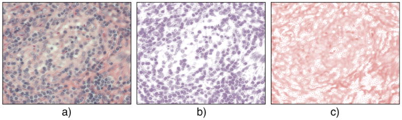
Color deconvolution example. MCL lymphoma sample stained with H&E combination in RGB (a). Deconvolved images in HE color space: H-channel (b) and E-channel (c).

D. Acquisition Specifics

Ten different cases of three different lymphomas (CLL, FL, MCL; 30 slides total) were imaged on a Zeiss Axioscope white light microscope with a 20x objective and a color CCD camera AxioCam MR5. The slides were imaged with the same instrument settings and same objective lens, camera, and light source. Therefore, no other normalization was performed for the camera channels.

Slides were selected with tumors present, providing representative cases, but information of the distribution of the malignant cells on the slides was not used. The slides were imaged randomly to avoid making assumptions about the distribution of malignancies. Tumor heterogeneity was expected to result in a different level or type of signal in different tiles within a complete image. A given image would have been classified correctly only if sufficient signal of the correct type was present in its constituent tiles. When reporting accuracy, we averaged the classifications of each of the constituent tiles and classified the entire image as one of the three lymphoma types. In this way, the heterogeneity of the tumor at the scale of individual tiles was downplayed relative to the scale of the whole field of view. Each image (1040 × 1388 pixels) was tiled into thirty sub-images on a 5× 6 grid with a tile size of 208 × 231 pixels. The number of images used for training was 57 (or 1710 image tiles) for each class, which is roughly six images (or 171 tiles) per slide. For testing there were 56, 82, and 65 images used for CLL, FL and MCL types, respectively.

IV. Statistical Classifiers Employed

In our experiments three classifiers capable of working with multi-category data were employed: Weighted Neighbor Distance (WND), naïve Bayes network (BBN) and radial basis functions (RBF). Previous experiments [11] demonstrated good performance of the WND classifier compared to state-of-the-art algorithms in a variety of imaging problems. Results from BBN and RBF classifiers are given for comparison. Feature ranking was applied to the global CHARM feature-set. While the BBN and RBF classifiers used ranking for conventional dimensionality reduction, the WND classifier used the feature weights to compute similarities to training classes.

A. WND Classifier

The general classification scheme in Fig. 3 uses the WND classifier. The WND algorithm relies on the sample-to-class distance ρ_c (t): ${\rho }_c(t)=\underset{j}{\mathrm{mean}}{\rho }_{\mathit{cj}}(t),{\rho }_{\mathit{cj}}(t)={\parallel {\overrightarrow{\delta }}_{\mathit{cj}}^w(t)\parallel }_2^2,c=1,..,C$, where the weighted difference δ⃗^w is ${\overrightarrow{\delta }}_{\mathit{cj}}^w=\overrightarrow{w}\cdot \left(\overrightarrow{t}-{\overrightarrow{X}}_j^{(c)}\right)$, and t⃗, ${\overrightarrow{X}}_j^{(c)}$ are the test and training samples, respectfully; C is the total number of classes. Note that in effect, ρ_c is the square of a Euclidean distance. Fisher scores [48] were used as weights in δ⃗^w, penalizing weak features and rewarding strong ones. Similarity of the sample t⃗ to the class c is defined as [11] $s_{\mathit{ci}}={\sum }_{j=1}^{N_c}{\rho }_{\mathit{cj}}^{-p}$, where N_c is the number of samples in the class c, and p is a parameter that provides an absorbing effect to individual variation. Although the parameter has rather broad range (from 0.01 to 20) with satisfactory classifier performance, we fixed it at 5. Experiments demonstrated that p = 5 works well in a range of different imaging applications [11]. The classification method calls the class c^pred when the similarity of the test sample is highest for this class, i.e. $c^{\mathrm{pred}}(\overrightarrow{t})=\underset{c}{\mathrm{arg\; max}}{s}_{\mathit{ci}}$. The probability of the sample t⃗ belonging to the class c^pred is defined as $P(t|c)={\rho }_{c^{\mathrm{pred}},i}/{\sum }_c{\rho }_{\mathit{ci}}$. This probability distribution represents the similarity of an individual test sample to each separate class.

Probabilities of each set of 30 tiles get averaged, and reported as the image probability distribution. Each image is assigned to a class based on the highest probability in the distribution. We made eight random splits of the image pool into training-test partitions and determined overall accuracy of the classifier as the average of the per-split performance scores (i.e., the accuracy is computed with an eight-fold cross-validation scheme).

B. Naïve Bayes and Radial Basis Functions

The Bayes classifier [48] is based on the concept of inference. The naïve Bayes classifier originates from applying the Bayes’ theorem with an assumption of independence of feature variables. The joint probability P(X₁, X₂,…, X_n|c) does not account for the interaction of variables, it is rather considered as a product of individual probabilities corresponding to different nodes of the Bayes network. We used the naïve Bayes classifier [49] that works with discrete data and employs a discretization algorithm [50] for adopting data to network inputs.

RBF network [48] has only two layers of nodes; it is easy to implement as no topology optimization is required. The top N features form the input layer. The network maps N - dimensional features to C dimensions of the predicted class. The network approximates the target function in the form $y_c(\overrightarrow{X})=\mathrm{\sum }_k{w}_k\varphi (\overrightarrow{X},{\overrightarrow{\mu }}_k)c=1,\dots ,C;y_c\in [0,1]$ with weights w_k and approximants ϕ (X⃗, μ⃗_k) (radial functions). Index c corresponds to c-th output variable, and μ⃗_k are the function centers. The Gaussian form of radial functions was used: $\varphi \left(\overrightarrow{X},{\overrightarrow{\mu }}_k\right)=\exp \left(-{\parallel \overrightarrow{X}-{\overrightarrow{\mu }}_k\parallel }_2^2/\left(2{\sigma }^2\right)\right)$, here σ were heuristically set to a multiple of the average distance between function centers of a corresponding class. The multivariate network output ${\left\{y_c\right\}}_{c=1}^C$ is subject to the constraint Σy_c = 1 that represents marginal probabilities.

V. Results

The HE set of channels (e.g., HE, H, and E) resulted in the best classification accuracy. Table III presents comparison of performances for a total of nine data sets (Gray, RGB, Red, Green, Blue, Lab, HE, H, and E) achieved using the three classifiers WND, BBN, and RBF. As Table III shows, the HE set of channels result in the best classification on three lymphomas (> 88% for BBN and > 98% for the other two classifiers), the RGB set gave the second-best result (90%), the Gray set produced second to worst accuracy (85%), while the Lab set gave the worst classification of all sets (maximum of 74%). We found that the WND classifier demonstrated the best overall performance with RBF performing very similarly, and with BBN never reporting the best accuracy.

TABLE III.

Data Set	WND-5	BBN	RBF
Gray	0.85 ± 0.03	0.72 ± 0.04	0.83 ± 0.06
RGB	0.90 ± 0.02	0.74 ± 0.06	0.87 ± 0.03
RGB, Red	0.84 ± 0.02	0.69 ± 0.03	0.86 ± 0.04
RGB, Green	0.81 ± 0.02	0.66 ± 0.04	0.77 ± 0.03
RGB, Blue	0.78 ± 0.01	0.61 ± 0.01	0.77 ± 0.02
Lab	0.74 ± 0.02	0.52 ± 0.05	0.71 ± 0.04
HE	0.98 ± 0.01	0.92 ± 0.03	0.98 ± 0.01
HE, E	0.99 ± 0.00	0.90 ± 0.06	0.99 ± 0.00
HE, H	0.98 ± 0.01	0.88 ± 0.05	0.98 ± 0.00

Performance comparison for different sets: WND, BBN, and RBF classifiers. Data in bold correspond to the strongest result for each data set.

One important property of a classifier is the number of features employed. In our experiments we found that WND worked most effectively in the range of 12-200 of the top-scoring features (scored by the methods described in Section II.E). Fig. 5 illustrates the convergence of accuracy as a function of number of features (N) for the WND classifier. As one can see in Fig. 5, the curve for HE channels remains flat for the entire range, while other color spaces show peaks and declines in accuracy for certain ranges of N. Also, N = 200 features are optimal only for the Lab set, while other sets require less than 100 features. BBN [49] worked optimally with as few as four top-scoring features. RBF worked best in relatively higher dimensional spaces: its accuracy peaked at about 400 features.

Fig. 5.

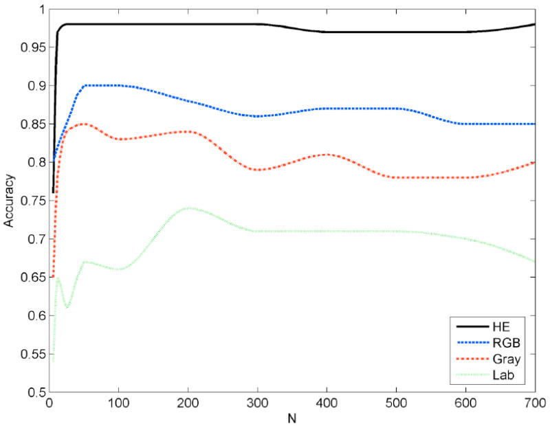
WND classifier accuracy for different number of features used in different color spaces (HE, RGB, Gray, and Lab).

Uniformity of per-class scoring is also a desirable property, and this was more significantly affected by the choice of color representation that it was by the choice of classifier. Table IV shows per-class accuracy for all nine data sets. The MCL class in Lab classified by WBD had a much lower accuracy (65%) than the other two classes (72% and 86% for CLL and FL respectively), affecting the uniformity of per-class scoring. In contrast, the MCL class in HE (98%), H (99%) and E (99%) was more accurately classified by WND than CLL (96%, 97%, 94% for HE, H and E respectively), and these three channels also gave the most uniform per-class scoring. This trend persisted in all three classifiers tested.

TABLE IV.

Data sets	CLL	FL	MCL
WND-5 classifier
Gray	0.91	0.90	0.75
Lab	0.72	0.86	0.65
RGB	0.86	0.97	0.87
RGB, Red	0.86	0.91	0.76
RGB, Green	0.80	0.89	0.73
RGB, Blue	0.82	0.86	0.66
HE	0.96	1.00	0.98
HE, H	0.97	1.00	0.99
HE, E	0.94	0.99	0.99
BBN classifier
Gray	0.77	0.85	0.52
Lab	0.39	0.75	0.41
RGB	0.80	0.90	0.49
RGB, Red	0.72	0.92	0.43
RGB, Green	0.62	0.86	0.50
RGB, Blue	0.71	0.73	0.39
HE	0.88	0.95	0.93
HE, H	0.80	0.87	0.96
HE, E	0.86	0.92	0.94
RBF classifier
Gray	0.85	0.88	0.78
Lab	0.70	0.82	0.60
RGB	0.85	0.91	0.84
RGB, Red	0.89	0.91	0.78
RGB, Green	0.83	0.81	0.67
RGB, Blue	0.85	0.86	0.60
HE	0.93	1.00	1.00
HE, E	0.98	0.99	1.00
HE, H	0.95	0.99	0.99

Per-class accuracies. With almost no exceptions, FL type demonstrates the best per-class performance in nearly all sets. For HE sets the performance for FL and MCL become very close.

We compared the effect of the three different feature ranking schemes described in the Section II.E on the three different classifiers in the HE color space (see Table V). We found that overall, FLD feature ranking demonstrated the best classification accuracy for all three classifiers. Table VI compares the effect of feature selection (FLD, F/C, and mRMR [32]) on the WND classifier in four color spaces (Gray, RGB, Lab, and HE) and shows that feature selection techniques do not have a marked effect on classification accuracy.

TABLE V.

Data sets	CLL	FL	MCL	Total
Fisher Discriminant
WND-5	0.96	1.00	0.98	0.98
BBN	0.88	0.95	0.93	0.92
RBF	0.93	1.00	1.00	0.98
Collinearity
WND-5	0.83	0.97	0.93	0.91
BBN	0.83	0.90	0.95	0.89
RBF	0.86	0.95	0.89	0.90
Pearson correlation
WND-5	0.79	1.00	0.94	0.91
BBN	0.73	0.83	0.94	0.83
RBF	0.88	0.98	0.99	0.95

Comparison of the three different feature ranking schemes (Fisher Scores, Colinearity Scores, and Pearson correlation). The HE data set was used. Fisher Scores gives the best accuracy of all three.

VI. Discussion

Results of automated lymphoma classification reported here on the three most prevalent malignancy types demonstrate the fruitfulness of whole-image pattern recognition without reliance on segmentation. The independence of this method from segmentation contributes to its potential generality, as previously demonstrated with its accuracy classifying many different image types both related and unrelated to histopathology. The absence of a segmentation step also allowed us to directly compare various color spaces for their information content as assayed by the classification accuracy of different down-stream dimensionality reduction and classification techniques.

The color spaces used in this study can be separated into three categories: original or camera-originated (R, G, B, and RGB); derived (Gray, Lab); and histological (HE, H, and E). For the original and derived categories it was observed that no single-channel data set could outperform the RGB set, where the WND accuracy is 90%. In contrast, the histological channels alone or in combination outperformed all other combinations of original and derived channels. It could be argued that the channels in the HE set are more orthogonal to each other than the channels in the RGB or Lab set because these color spaces are convolutions of the different information represented by the separate H and E stains, mainly nuclei and cytoplasm. The features computed from the HE channels would then be more unrelated to each other and thus represent a greater variety of image content than features computed from the RGB channels, each of which contains both H and E in different proportions.

The orthogonality of color channels cannot explain the poor performance of Lab compared to RGB. The Lab color space was designed as an orthogonal color space specifically to allow measuring Euclidean distances between colors. At the same time, the transformation between RGB and Lab is reversible, meaning that it preserves all information content. Yet Lab had the worst performance of all color spaces tried. In contrast, the Gray transformation from RGB is clearly not reversible and represents information loss, and yet Gray performed better than Lab. The performance of Gray relative to Lab also contradicts the argument that more channels result in better performance, even though this was observed for RGB relative to R, G and B separately. These observations indicate that neither diversity nor quantity, or even completeness is sufficient to yield the best classification results.

When pathologists classify these samples, they tend to identify landmarks, similarly to the segmentation process in machine vision. They tend to use several magnifications to aid in identifying these landmarks, and focus their attention on particular areas of tissue for a small number of diagnostic markers. In contrast, whole-image pattern recognition seems to be entirely unrelated to this process as it doesn’t use segmentation, processes random collections of images, and relies on many weakly-discriminating features in concert to achieve a diagnosis. Our observations of classification accuracy in different color domains indicate that those domains that are best at preserving biological morphology (HE, H, and E) perform best in direct comparisons. Despite the differences between how machines and pathologists process visual information, it is apparently the preservation of biologically relevant cellular morphology that allows machines to achieve the best classification results.

VII. Future Work

Our ultimate goal is a diagnosis of new cases on previously unseen slides. The major difficulty of this objective is the variability of existing data: the slide collection used in this study contains a broad range of variables including different sectioning and staining performed at different clinics. We believe that standardization in sample preparation is an important factor in machine-assisted or automated diagnostic histopathology just as it is for manual diagnosis [51, 52]. In future studies we will evaluate the performance of this classifier on tissue micro-arrays (TMAs), where biopsies from different patients and hospitals can be arrayed on the same slide and stained in bulk to eliminate much of this variability. While TMAs may themselves not be practical in a clinical setting, a demonstration that a more uniform sample produces more accurate diagnosis will encourage the standardization of these processing techniques.

In this study we revealed image processing factors that promote separability of the three major types of lymphoma. In a more clinical setting, additional considerations would have to be accounted for, including a greater diversity of cases as well as an expansion in the number of different lymphomas to be analyzed. In a clinical application, pattern recognition systems can be used in various capacities ranging from stand-alone to decision support. Even a limited system like that presented here has the benefit of consistency, and so can act to reduce the degree of variation in classification ability of different pathologists.

VIII. Conclusions

A whole-image pattern recognition method can be successful in discriminating between three of the most common lymphoma types. A classification accuracy of 99% is possible without segmentation, using multiple magnifications, or selecting training images containing diagnostic lymphoma markers. The strongest signal is contained in a histological (HE) color scheme, with the original (RGB) scheme giving measurably worse performance, indicating that classification is sensitive to biologically relevant morphologies.

References

- 1.Harris NL, Jaffe ES, Diebold J, Flandrin G, Muller-Hermelink HK, Vardiman J, Lister TA, Bloomfield CD. The World Health Organization classification of neoplastic diseases of the hematopoietic and lymphoid tissues. Report of the Clinical Advisory Committee meeting, Airlie House, Virginia, November, 1997. Ann Oncol. 1999 Dec;10:1419–32. doi: 10.1023/a:1008375931236. [DOI] [PubMed] [Google Scholar]
- 2.Jemal A, Siegel R, Ward E, Hao Y, Xu J, Murray T, Thun MJ. Cancer statistics, 2008. CA Cancer J Clin. 2008 Mar-Apr;58:71–96. doi: 10.3322/CA.2007.0010. [DOI] [PubMed] [Google Scholar]
- 3.Armitage JO, Bierman PJ, Bociek RG, Vose JM. Lymphoma 2006: classification and treatment. Oncology (Williston Park) 2006 Mar;20:231–9. discussion 242, 244, 249. [PubMed] [Google Scholar]
- 4.Rodenacker K, Bengtsson E. A feature set for cytometry on digitized microscopic images. Analytic cellular pathology. 2003;25:1–36. doi: 10.1155/2003/548678. [DOI] [PMC free article] [PubMed] [Google Scholar]
- 5.Tabesh A, Teverovsky M, Pang HY, Kuar VP, Verbel D, Kotsianti A, Saidi O. Multifeature prostate cancer diagnostics and Gleason grading of histological images. IEEE Transactions on Medical Imaging. 2007;26:1366–1378. doi: 10.1109/TMI.2007.898536. [DOI] [PubMed] [Google Scholar]
- 6.Murphy RF. Automated interpretation of protein subcellular location patterns: implications for early detection and assessment. Annals of the New York Academy of Sciences. 2004;1020:124–131. doi: 10.1196/annals.1310.013. [DOI] [PubMed] [Google Scholar]
- 7.Sertel O, Kong J, Lozanski G, Shana’ah A, Catalyurek U, Saltz J, Gurcan M. Texture classification using non-linear color quantization:Application to histopathological image analysis. Proceedings of IEEE International Conference on Acoustics, Speech and Signal Processing (ICASSP 2008); Las Vegas, NV. 2008. [Google Scholar]
- 8.Nielsen B, Albregsten F, Danielsen H. Low dimensionality adaptive texture feature vectors from class distance and class difference matrices. IEEE Transactions on Medical Imaging. 2004;23:73–84. doi: 10.1109/TMI.2003.819923. [DOI] [PubMed] [Google Scholar]
- 9.Tuzel O, Yang L, Meer P, Foran D. Classification of hematologic malignancies using texton signatures. Pattern Analysis and Applications. 2007 Mar;10:277–290. doi: 10.1007/s10044-007-0066-x. [DOI] [PMC free article] [PubMed] [Google Scholar]
- 10.Nava VE, Jaffe ES. The pathology of NK-cell lymphomas and leukemias. Advances in Anatomy and Pathology. 2005 Jan;12:12–34. doi: 10.1097/01.pap.0000151318.34752.80. [DOI] [PubMed] [Google Scholar]
- 11.Orlov N, Shamir L, Macura T, Johnston J, Eckley DM, Goldberg IG. WND-CHARM: Multi-purpose image classification using compound image transforms. Pattern Recognition Letters. 2008;29:1684–1693. doi: 10.1016/j.patrec.2008.04.013. [DOI] [PMC free article] [PubMed] [Google Scholar]
- 12.Orlov N, Johnston J, Macura T, Shamir L, Goldberg I. Computer Vision for Microscopy Applications. In: Obinata G, Dutta S, editors. Vision Systems: Segmentation and Pattern Recognition. Vienna, Austria: I-Tech Education and Publishing; 2007. pp. 221–242. [Google Scholar]
- 13.Johnston J, Iser WB, Chow DK, Goldberg IG, Wolkow CA. Quantitative image analysis reveals distinct structural transitions during aging in Caenorhabditis elegans tissues. PLoS ONE. 2008;3:e2821. doi: 10.1371/journal.pone.0002821. [DOI] [PMC free article] [PubMed] [Google Scholar]
- 14.Orlov N, Johnston J, Macura T, Wolkow C, Goldberg I. Pattern recognition approaches to compute image similarities: application to age related morphological change. International Symposium on Biomedical Imaging: From Nano to Macro; Arlington, VA. 2006. pp. 1152–1156. [Google Scholar]
- 15.Shamir L, Ling SM, Scott W, Orlov N, Macura T, Eckley DM, Ferrucci L, Goldberg IG. Knee X-ray image analysis method for automated detection of Osteoarthritis. IEEE Transactions on Biomedical Engineering. 2009 Feb;56:407–415. doi: 10.1109/TBME.2008.2006025. [DOI] [PMC free article] [PubMed] [Google Scholar]
- 16.Shamir L, Ling SM, Scott W, Hochberg M, Ferrucci L, Goldberg IG. Early Detection of Radiographic Knee Osteoarthritis Using Computer-aided Analysis. Osteoarthritis and Cartilage. 2009 doi: 10.1016/j.joca.2009.04.010. in press. [DOI] [PMC free article] [PubMed] [Google Scholar]
- 17.Shamir L, Ling S, Rahimi S, Ferrucci L, Goldberg IG. Biometric identification using knee X-rays. International Journal of Biometrics. 2009;1:365–370. doi: 10.1504/IJBM.2009.024279. [DOI] [PMC free article] [PubMed] [Google Scholar]
- 18.Shamir L, Orlov N, Mark Eckley D, Macura TJ, Goldberg IG. IICBU 2008: a proposed benchmark suite for biological image analysis. Med Biol Eng Comput. 2008 Sep;46:943–7. doi: 10.1007/s11517-008-0380-5. [DOI] [PMC free article] [PubMed] [Google Scholar]
- 19.Foran D, Comaniciu D, Meer P, Goodel L. Computer-assisted discrimination among malignant lymphomas and leukemia using immunophenotyping, intelligent image repositories, and telemicroscopy. IEEE Transactions on Information Technology in Biomedicine. 2000 Dec;4:265–273. doi: 10.1109/4233.897058. [DOI] [PubMed] [Google Scholar]
- 20.Tagaya R, Kurimoto N, Osada H, Kobayashi A. Automatic objective diagnosis of lymph nodal disease by B-mode images from convex-type echobronchoscopy. Chest. 2008;133:137–142. doi: 10.1378/chest.07-1497. [DOI] [PubMed] [Google Scholar]
- 21.Monaco J, Tomaszewski J, Feldman M, Mehdi M, Mousavi P, Boag A, Davidson C, Abolmaesumi P, Madabhushi A. Probabilistic Pair-wise Markov Models: Application to Prostate Cancer Detection. Medical Imaging 2009: Image Processing. 2009:1–12. [Google Scholar]
- 22.Rosenfeld A. From image analysis to computer vision: an annotated bibliography, 1955-1979. Computer Vision and Image Understanding. 2001;84:298–324. [Google Scholar]
- 23.Duda R, Hart P, Stork D. Pattern classification. 2. New York, NY: John Wiley & Sons; 2001. [Google Scholar]
- 24.Gonzalez R, Wood R. Digital image processing. Reading, MA: Addison-Wesley Publishing Company; 2007. [Google Scholar]
- 25.Wang L. Feature selection with kernel class separability. IEEE Trans on Pattern Analysis and Machine Intelligence. 2008;30:1534–1546. doi: 10.1109/TPAMI.2007.70799. [DOI] [PubMed] [Google Scholar]
- 26.Frigo M, Johnston SG. The design and implementation of FFTW3. Proceedings of the IEEE. 2005;93:216–231. [Google Scholar]
- 27.Gurevich IB, Koryabkina IV. Comparative analysis and classification of features for image models. Pattern Recognition and Image Analysis. 2006;16:265–297. [Google Scholar]
- 28.Marsolo K, Twa M, Bullimore M, Parthasarathy S. Spatial modeling and classification of corneal shape. IEEE Transactions on Information Technology in Biomedicine. 2007 Mar;11:203–212. doi: 10.1109/titb.2006.879591. [DOI] [PubMed] [Google Scholar]
- 29.Theera-Umpton N, Dhompongsa S. Morphological granulomitric features of nucleus in automatic bone marrow white blood cell classification. IEEE Transactions on Information Technology in Biomedicine. 2007 May;11:353–359. doi: 10.1109/titb.2007.892694. [DOI] [PubMed] [Google Scholar]
- 30.Lu C, Devos A, Suykens JA, Arus C, Huffel SV. Bagging linear sparse Bayesian learning models for variable selection in cancer diagnosis. IEEE Transactions on Information Technology in Biomedicine. 2007 May;11:338–347. doi: 10.1109/titb.2006.889702. [DOI] [PubMed] [Google Scholar]
- 31.Shamir L, Wolkow CA, Goldberg IG. Quantitative measurement of aging using image texture entropy. Bioinformatics. 2009 doi: 10.1093/bioinformatics/btp571. in press. [DOI] [PMC free article] [PubMed] [Google Scholar]
- 32.Peng H, Long F, Ding C. Feature selection based on mutual information: criteria of max-dependency, max-relevance, and min-redundancy. IEEE Tr on Pattern Analysis and Machine Intelligence. 2005;27:1226–1238. doi: 10.1109/TPAMI.2005.159. [DOI] [PubMed] [Google Scholar]
- 33.Gupta D, Lim MS, Medeiros LJ, Elenitoba-Johnson KSJ. Small lymphosytic lymphoma with perifollicular, marginal zone, or interfollicular distribution. Modern Pathology. 2000;13:1161–1166. doi: 10.1038/modpathol.3880214. [DOI] [PubMed] [Google Scholar]
- 34.Kimm LR, Deleeuw RJ, Savage KJ, Rosenwald A, Campo E, Delabie J, Ott G, Muller-Hermelink HJ, Jaffe ES, Rimsza LM, Wersenburger DD, Chan WC, Staudt LM, Connors JM, Gascoyne RD, Lam WL. Frequent occurences of deletions in primary mediastinal B-cell lymphoma. Genes Chromosomes Canser. 2007 Dec;46:1090–1097. doi: 10.1002/gcc.20495. [DOI] [PubMed] [Google Scholar]
- 35.Cuadros M, Dave SS, Jaffe ES, Honrado E, Milne R, Alves J, Rodriguez J, Zajac M, Benitez J, Staudt LM, Martinez-Delgado B. Identification of a proliferation signature related to survival in nodal periipheral T-cell lemphomas. Journal of Clinical Oncology. 2007 Aug;25:3321–3329. doi: 10.1200/JCO.2006.09.4474. [DOI] [PubMed] [Google Scholar]
- 36.Paschos G, Petrou M. Histogram ratio features for color texture classification. Pattern Recognition Letters. 2003;24:309–314. [Google Scholar]
- 37.Gauch JM, Shivadas A. Finding and identifying unknown commercials using repeated video sequence detection. Computer Vision and Image Understanding. 2006;103:80–88. [Google Scholar]
- 38.Arvis V, Debain C, Berducat M, Benassi A. Generalization of the cooccurance matrix for colour images: application to colour texture classification. Image Analysis & Stereology. 2004;23:63–72. [Google Scholar]
- 39.Sertel O, Kong J, Catalyurek UV, Lozanski G, Saltz JH, Gurcan MN. Histopathological image analysis using modelbased intermediate representations and color texture: follicular lymphoma grading. Journal of Signal Processing Systems. 2009;55:169–183. [Google Scholar]
- 40.Kong J, Shimada H, Boyer K, Saltz J, Gurcan MN. Image analysis for automated assessment of grade of neuroblastic differentiation. IEEE ISBI2007: International Symposium on Biomedical Imaging: From nano to macro; Metro Washington, D.C. 2007. [Google Scholar]
- 41.Cooper L, Sertel O, Kong J, Lozanski G, Huang K, Gurcan M. Feature-based registration of histopathology images with different stains: An application for computerized follicular lymphoma prognosis. Computer Methods and Programs in Biomedicine. 2009;96:182–192. doi: 10.1016/j.cmpb.2009.04.012. [DOI] [PMC free article] [PubMed] [Google Scholar]
- 42.Xu J, Tu L, Zhang Z, Qiu X. A medical image color correction method base on supervised color constancy. IEEE International Symposium on IT in Medicine and Education; Xiamen, China. 2008. [Google Scholar]
- 43.Van de Ville D, Philips W, Lemahieu I, Van de Walle R. Suppression of sampling moire in color printing by spline-based least-squares prefiltering. Pattern Recognition Letters. 2003;24:1787–1794. [Google Scholar]
- 44.Acharya T, Ray KK. Image processing: principles and applications. Wiley Interscience; 2005. [Google Scholar]
- 45.Wyszecki G, Stiles WS. Color science: concepts and methods, quantitative data and formulae. 2. New York: John Wiley & Sons; 1982. [Google Scholar]
- 46.Verikas A, Gelziniz A, Bacauskiene M, Uloza V. Towards a computer-aided diagnosis system for vocal cord diseases. Artificial Intelligence in Medicine. 2006;36:71–84. doi: 10.1016/j.artmed.2004.11.001. [DOI] [PubMed] [Google Scholar]
- 47.Ruifrok AC, Johnston DA. Quantification of histochemical staining by color deconvolution. Anal Quant Cytol Histol. 2001 Aug;23:291–299. [PubMed] [Google Scholar]
- 48.Bishop C. Neural networks for pattern recognition. Oxford University Press; 1996. [Google Scholar]
- 49.Murphy K. The Bayes net toolbox for Matlab. Computing Science and Statistics. 2001;33:1–20. [Google Scholar]
- 50.Dougherty J, Kohavi R, Sahami M. Supervised and unsupervised discretization of continuous features. Proceedings of the 12th International Conference on Machine Learning; Tahoe City, CA. Morgan Kaufmann; 1995. pp. 194–202. [Google Scholar]
- 51.Vinh-Hung V, Bourgain C, Vlastos G, Cserni G, De Ridder M, Storme G, Vlastos A-T. Prognostic value of histopathology and trends in cervical cancer: a SEER population study. BMC Cancer. 2007 Aug;7:1–13. doi: 10.1186/1471-2407-7-164. [DOI] [PMC free article] [PubMed] [Google Scholar]
- 52.Drake TA, Braun J, Marchevsky A, Kohane IS, Fletcher C, Chueh H, Beckwith B, Berkowicz D, Kuo F, Zeng QT, Balis U, Holzbach A, McMurry A, Gee CE, McDodald CJ, Schadow G, Davis M, Hattab EM, Blevins L, Hook J, Becich M, RS C, Taube SE, Berman J. Shared pathology informatics network. Human Pathology. 2007 Aug;38:1212–1225. doi: 10.1016/j.humpath.2007.01.007. [DOI] [PubMed] [Google Scholar]