Forecasting ICP Elevation Based on Prescient Changes of Intracranial Pressure Waveform Morphology

Abstract

Interventions of intracranial pressure (ICP) elevation in neurocritical care is currently delivered only after healthcare professionals notice sustained and significant mean ICP elevation. The present work used the Morphological Clustering and Analysis of Intracranial Pressure (MOCAIP) algorithm to derive 24 metrics characterizing morphology of ICP pulses and tested the hypothesis that pre-intracranial hypertension (pre-IH) segments of ICP can be differentiated, using these morphological metrics, from control segments that were not associated with any ICP elevation. Furthermore, we investigated whether a global optimization algorithm could effectively find the optimal sub-set of these morphological metrics to achieve better classification performance as compared to using full set of MOCAIP metrics. The results showed that Pre-IH segments, using the optimal sub-set of metrics found by the differential evolution (DE) algorithm, can be differentiated from control segments at a specificity of 97% and sensitivity of 78% for those Pre-IH segments 5 minutes prior to the ICP elevation. While the sensitivity decreased to 68% for Pre-IH segments 20 minutes prior to ICP elevation, the high specificity remained. The performance using the full set of MOCAIP metrics was shown inferior to results achieved using the optimal sub-set of metrics. The present work demonstrated that advanced ICP pulse analysis combined with machine learning could potentially lead to the forecasting of ICP elevation so that a proactive ICP management could be realized based on these accurate forecasts.

1. Introduction

Intracranial pressure (ICP) elevation occurs frequently in traumatic brain injury (TBI) and aneurysmal subarachnoid hemorrhage (aSAH) patients as well as in some patients with idiopathic headache. This condition needs immediate treatment for preventing secondary brain injury in patients undergoing intensive care. Invasive ICP monitoring remains the gold standard adopted by clinicians for detecting ICP elevation. However, the detection of ICP elevation is established primarily by noticing mean ICP changes. Typically, reactive measures are taken, such as drainage of ventricular cerebrospinal fluid (CSF) or administering osmotic diuretics, if the mean ICP exceeds a set value for longer than a defined duration (typically 20 mm Hg for 5 minutes)[1]. Relying solely on mean ICP is an accurate way of detecting ICP elevation but it may carry a significant risk of delaying the treatment. The delays from the occurrence of ICP elevation to its successful abatement may be caused by failure to notice the mean ICP change, the five-minute observing period, and the delay for any treatment to take effect. Given the significance and success of ICP management in improving patient outcome for brain injury patients, it is thus a significant endeavor to further optimize the detection process of ICP elevation so that a more proactive ICP management can be achieved to reduce the aforementioned time delay.

Given the continuous nature of ICP monitoring, a viable way of improving ICP elevation detection is to establish precursors to ICP elevation that can be extracted from continuous ICP signals so that pending ICP elevation can be recognized prior to its occurrence. In an early study, several ICP metrics other than mean ICP were investigated for differentiating the transient ICP elevation from refractory ICP elevation[2]. Despite this study was not conducted from the perspective of searching for precursors of ICP elevation, it resembles one of the early attempts to extract additional ICP metrics beyond mean ICP for classifying different ICP patterns. ICP plateau wave as described in the original publication in 1960s[3] is a severe form of ICP elevation. Czosnyka et al. studied the hemodynamic and intracranial volumetric compensatory characteristics associated with the ICP plateau wave[4]. It was found in this study that ICP plateau wave was associated with a preserved cerebral blood flow (CBF) autoregulation and decreased intracranial volumetric compensatory reserve. However, no further effort has been reported to investigate whether these characteristics can be used as unique precursors of ICP elevation. A more recent effort[5] applied statistical signal analysis methods to search for precursors of acute ICP elevation. However, no clue about the specificity of the studied ICP metrics can be obtained from this preliminary study. Further efforts in searching for precursors of ICP elevation were also conducted using advanced signal analysis methods originated in the field of nonlinear dynamic analysis of time series. Approximate entropy is a widely used metric for characterizing the complexity of a time series and was applied to study ICP elevation where it was found that both ICP pulse[6] and slow-wave components of ICP signals[7] showed a decreasing trend of complexity prior to ICP elevation. However, no further effort has been found in quantifying how unique the observed complexity decreasing of ICP signals is related to ICP elevation. Another attempt towards early recognition of ICP elevation was reported in a recent publication[8] where a single ICP metric was studied, which quantifies the ratio between the amplitudes of the second and the first sub-peaks of an ICP pulse. This P₂/P₁ ratio was chosen to hopefully capture a long-established phenomena associated with ICP elevation, i.e., the rounding of ICP pulse as ICP elevation develops. However, disappointing results were reported that elevation of P₂/P₁ ratio above 0.8 was not uniquely associated with ICP elevation because it was also observed in TBI patients without any episodes of ICP elevation.

In summary, there exist prior efforts on researching precursors to ICP elevation. However, a commonly missed item in these previous studies is the incorporation of an experiment that can quantitatively assess the quality of proposed precursors in terms of the important performance metrics including sensitivity, specificity, and positive predictivity. Apart from this, a comprehensive and systematic analysis of ICP signal is needed for extracting precursors that are beyond what have been reported so far. The present work attempts to move forward the frontier of research in predicting ICP elevation by addressing these two issues.

We have recently proposed and validated a method to analyze ICP pulse morphology[9]. This algorithm can reliably identify the three well-established sub-peaks of a processed ICP pulse so that its morphology can be characterized using a comprehensive set of metrics to be introduced in next Section. Our attention to a possible utilization of ICP morphological metrics for predicting ICP elevation is justified by the long-established phenomenon of ICP pulse transiting from a normal 3-peak configuration to a more rounding form as ICP elevation develops. This new algorithm has provided a more comprehensive set of metrics for a complete characterization of these morphological changes than what have been reported in this field [2, 8, 10, 11]. Therefore, our hypothesis is that ICP elevation can be forecasted by morphological changes, captured by this new algorithm, of ICP pulses preceding the eventual increase of ICP.

The remaining challenge is therefore related to how an experiment can be set up to systematically test this hypothesis. We selected a dataset that contains data of both types of patients: one with ICP elevation and controls without any ICP elevation episodes from a group of non-traumatic brain injury patients (idiopathic intracranial hypertension, Chiari syndrome, and slit ventricle patients with clamped shunts) with known risks of intracranial pressure elevation. Then all ICP elevation episodes were found by manual screening. Corresponding control episodes were generated in a random and unbiased way from control patients as well as from the recordings at least one hour ahead of the start of ICP elevation. With this data set constructed, we can then proceed with a classic cross-validation experiment on evaluating the performance of a two-class classifier to establish the quantitative metrics of how well ICP elevation and its pre-elevation episodes can be differentiated from normal control episodes. With these metrics, one could objectively assess the ICP prediction problem itself and the usefulness of the ICP pulse morphological metrics.

2. Methods

2.1 Patient and Data Preparation

The study cohort consisted of 36 subjects selected from 38 patients undergoing continuous intracranial pressure monitoring at the UCLA Medical Center for: 1) headache evaluation in patients with suspected idiopathic intracranial hypertension or shunt malfunction, and 2) management of adult slit ventricle syndrome in which CSF flow from an externalized CSF shunt was purposefully stopped. 3) pre- or post-treatment of Chiari. Based on our experience, spontaneous intracranial hypertension can occur for all three patient populations. Two patients were excluded because no waveform data archival for them could be found.

The ICP recordings were screened to identify episodes of intracranial hypertension defined as elevated ICP (> 20 mmHg) over a period of at least five minutes. As a result, we found 13 patients who had at least one such intracranial hypertension episode and the total number of episodes is 70. Five patients had 1 episode, one patient had 2 episodes, and three patients had 4 episodes of ICP elevation. The number of IH episodes for the remaining four patients is 7, 8, 14, and 22, respectively. These include 6 headache, 6 slit ventricle, and 1 Chiari patient.

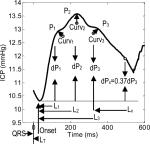
Based on the manually tagged starting positions of ICP elevation episodes, signal segments prior to Intracranial Hypertension (termed pre-IH segments) were generated based on five timing choices as illustrated in Fig.1. The length of each segment is 3 minutes long. For segment Pre-IH(0), we started data selection two minutes past the annotated starting positions of ICP elevation. For the rest of the Pre-IH segments, we started selection 4.5 minutes prior to the chosen timing point so that there is a 1.5 minutes interval from the last sample of the selection to the timing points. Based on this schema, we generated 70 Pre-IH(0), 67 Pre-IH(5), 66 Pre-IH(10), 62 Pre-IH(15), and 54 Pre-IH(20) segments. The number of selected Pre-IH segments decreases because ICP elevation could recur at a frequency shorter than the prescribed timing interval to the start of ICP elevation.

Figure 1.

Illustration of constructing pre-intracranial hypertension segments at different time intervals relative to the start of ICP elevation for an episode of ICP plateau wave.

Two types of control episodes were generated. We first chose a random 3-minute noise-free ICP segment for every 30 minutes of ICP recordings of the 23 control patients who did not have a single episode of ICP elevation. The total number of such control segments is 234. The second control set was constructed in a similar fashion but from ICP recordings that were at least one hour prior to ICP elevation episodes. This resulted in 166 segments. Then both types of control episodes were mixed as the final control set. It should be noted that the evaluation of classification perform in the present work was segment-based as it is relevant to detect the occurrence of each ICP elevation episode.

Each of these 3-minute segments was then processed by the ICP pulse analysis algorithm to be described in next sub-section that resulted in 24 morphological metrics listed in Table 1.

Table 1.

Illustration of ICP MOCAIP metrics that can be extracted by the current MOCAIP algorithm.

	MOCAIP Metric Group		Metrics
	Amplitude	Absolute	mICP, dP1, dP2, dP3, diasICP
		Ratio	dP2/ dP1(dP12), dP3/ dP1(dP13), dP3/ dP2(dP23)
	Time Interval	Absolute	LT, L1, L2, L3
		Relative	L2 - L1(L12), L3 - L1(L13), L3 - L2(L23)
	Pulse Curvature	Absolute	Curv1, Curv2, Curv3, Curvm
		Ratio	Curv2/ Curv1(Curv12), Curv3/ Curv1(Curv13), Curv3/ Curv2(Curv23)
	Slope		(P1- diasICP)/ L1 (k1)
	Decay time constant		Lx where dPx = 0.37 dP3

This retrospective analysis of the data set was approved by the Institutional Review Board committee of the UCLA Medical Center.

2.2 MOCAIP Algorithm

We developed a technique[9, 12], termed Morphological Clustering and Analysis of Intracranial Pressure (MOCAIP), for recognizing the locations of the three ICP sub-peaks and then calculating the 24 MOCAIP metrics illustrated in Table 1. These metrics allows a comprehensive quantitative characterization of ICP pulse morphology including pulse amplitude, time intervals among sub-peaks, curvature, slope, and decay time constants. Briefly, this technique accomplishes this detailed analysis of ICP pulse by sampling a discrete period of a digital ICP recording, and then in order: 1) performing individual ICP pulse detection, 2) segregating ICP pulses using cluster analysis, and then 3) rejecting individual illegitimate (incomplete, bizarre, etc) waveforms. The latter step is facilitated by comparison to a library of legitimate ICP pulses derived from our large patient database as described in[9]. Representative ICP waveforms from each cluster group are derived by an averaging process, which greatly improves the signal-to-noise ratio. The representative waveform from this dominant cluster is then used for sub-peak detection and designation.

Pulse Detection

We adopted a previously developed method for detecting each ICP pulse[13] using both ECG and ICP signals. As a result, the start of individual ICP pulses is defined at the corresponding QRS peak of ECG.

Pulse Clustering

Clinical ICP recordings are often contaminated by noise and artifacts including instrument noise, transient perturbation, sensor detachment, and quantization noise by the digitization process. These noises and artifacts result in poor quality of individual ICP pulses hampering a detailed analysis of their morphological features. We therefore reason that a sensible tradeoff can be made to conduct the analysis of ICP pulse morphology by not using individual pulse but rather using a representative cleaner pulse to be extracted from a sequence of consecutive raw ICP pulses. The MOCAIP algorithm uses a clustering method to extract this representative ICP pulse. A sequence of raw ICP pulse is first clustered into distinct groups based on their morphological distance. The largest cluster is then identified. An averaging process is conducted to obtain an averaged pulse for this largest cluster. In the context of MOCAIP, we call this average pulse of the largest cluster the dominant ICP pulse. Subsequent analysis of ICP morphology will be only conducted for this dominant pulse.

Legitimate Pulse Recognition

A dominant pulse is immune to noises of transient natures. However, it could still be artifactual because the complete segment it represents could be noise, e.g., sensor detachment can cause several minutes or even hours of ICP recording to be invalid. To identify legitimate dominant ICP pulses in an automated fashion, we propose to use a reference library of validated ICP pulses to aid the recognition of non-artifactual ones. This library of reference ICP pulses was constructed with legitimate pulses of diverse shapes as described in our original publication[9].

Detection of ICP Sub-peaks

Instead of using the strict condition x_i–1 < x_i < x_i+1 to define position i as a peak, the MOCAIP algorithm performs a comprehensive search for all landmark points on an ICP pulse as candidates for designating the three sub-peaks. For notational simplicity, these landmarks are still called peaks in MOCAIP. The first step to find the landmarks is to find the second derivative of an ICP pulse. Based on the sign of the second derivative, an ICP pulse can be segmented into concave and convex regions. We treat the intersection of a concave to a concave region on the ascending portion of the pulse as a landmark. On the descending portion of the pulse, the intersection of a convex to a concave region is treated as a landmark.

Assignment of Detected Peaks

The objective of this last step of the MOCAIP algorithm is to obtain the best designation of the three well-recognized ICP sub-peaks, denoted as P₁, P₂, and P₃ respectively, from an array of detected candidate peaks plus an empty designation. Let a₁, a₂,..., a_N represent an array of N detected peak candidates and a₀ represent an empty designation such that if a₀ is assigned to one of P₁, P₂, and P_3, it means that no corresponding sub-peak is present. The solution to this peak designation problem is found by a divide-and-conquer procedure that selects the optimal configuration based on the prior distributions of each of the three peaks as determined from the same ICP reference pulse library.

2.3 Calculating MOCAIP metrics for pulses with less than three peaks

For a small number of segments whose number of sub-peaks is less than three, we adopted the following simple rules to calculate the morphological metrics: 1) If only P₁ is missing, we consider P₁ and P₂ coincide; 2) if only P₂ is missing, we consider P₁ and P₂ coincide; 3) if only P₃ is missing, we consider P₂ and P₃ coincide; 4) if only one peak is present, we consider that all three peaks are merged into one.

2.4 Classification Experiment

We designed a classification experiment to test the hypothesis that Pre-IH ICP waveform as selected in Section 2.1 can be differentiated from ICP waveform from controls. This is essentially a two-class classification problem and we adopted the four conventional measures to quantify the classification performance. These measures include sensitivity (Sen), specificity (Spe), positive predictivity (PPV), and accuracy (AC). A simple regularized quadratic discriminator[14] was chosen as the classifier. Apart from these standard elements of a classification experiment design, a novel aspect of the present study was that we used an optimal feature selection algorithm to automatically select the best combination of MOCAIP metrics as an input feature vector to the quadratic decision function.

As no prior knowledge is available with regard to what constitutes the most useful MOCAIP metrics for differentiating Pre-IH and control segments, one attempt is to use the full set of MOCAIP metrics to compose a feature vector. The risk of doing so is that the correlation among MOCAIP metrics will decrease classification performance, especially when the classifier is trained over a finite set of training data. In addition, the classification problem is unnecessarily complicated by having a high-dimensional feature vector.

Therefore, an automated and unbiased feature selection process is necessary. Indeed, this process can be abstracted as an optimization process. The variable to be optimized is the combination of MOCAIP metrics and the objective function can be constructed as a function of classification performance measures. The challenge to find the optimal solution is the inhibitive computational cost if a brute force search over set of candidate solutions is taken. Given 24 MOCAIP metrics, there will be ${\sum }_{i=1}^{23}{C}_{23}^i-1=8388607$ possible combinations of MOCAIP metrics to comprise a feature vector. Due to this huge number of possible solutions, brute force search is therefore not an option.

Instead, we adopted an efficient global random search strategy called differential evolution (DE) [15] to locate the best possible solution within a finite amount of time. Our previous experience [16] with the DE algorithm indicates that it is a highly efficient global search algorithm so that one can reasonably be certain that the solution provided by the DE is probably the best possible one given an equivalent computational expenditure to other search algorithms.

We chose the average of the sensitivity and positive predictivity as the objective function for the DE algorithm to maximize, whose values are found by the standard leave-one-patient-out cross-validation procedure [14].

A binary encoding schema was chosen to represent whether a MOCAIP metric is selected using a real number between [0, 1] so that any value ≥ 0.5 would indicate that the corresponding metric is selected. In addition, the regularized quadratic classifier has two tunable parameters whose range is also [0, 1]. We incorporated these two parameters into the optimization process as well. In summary, there are 24 variables to be optimized for classifying Pre-IH(0) from normal controls that include 22 MOCAIP metrics and two tunable parameters for the regularized quadratic classifier. Mean and diastolic ICP have to be excluded as part of the classier features for classifying Pre-IH(0) because mean ICP should be elevated already. For classifying the rest of Pre-IH segments, all 24 MOCAIP metrics can be engaged and hence the dimension of the variable to be optimized is 26.

After finding the best combination of MOCAIP metrics and the optimal values for the two classifier parameters, we used a standard bootstrapping cross-validation procedure[14] to evaluate the performance of classification under this optimal setup. To investigate the variability of this classification experiment, we independently run the above the optimization and bootstrapping processes for five times.

As a comparison, we also evaluated the classification performance using the full set of MOCAIP metrics as the feature vector. In this case, the two tunable parameters of the regularized quadratic classifier were still optimized using the DE algorithm.

2.5 Simulating online execution of the algorithm

Despite our focus in the present work is the classification of different pre-IH segments against the control segments, it is necessary to do a preliminary assessment of forecasting ICP elevation in a real-scenario using the proposed classification algorithm. This was done as the follows. We arbitrarily chose the optimal MOCAIP metrics combination and classifier parameters found in the first of the five classification experiments conducted at each Pre-IH segment. For the reason of prediction, we excluded Pre-IH(0). We then collected all available data for 23 control patients and 13 patients with IH. The MOCAIP algorithm was executed for every 3-minute non-overlapped signal segment of these data and the quality of the dominant pulse was visually evaluated to exclude all noisy 3-minute segments.

Then a leave-one-out schema was adopted to construct classifiers and test them on the these 3-minute segments, i.e., the four Pre-IH classifiers were constructed by excluding training data that are from the patient being tested. We report the performance of in terms of false positive rate, hourly false positive count, and sensitivity. Two types of control segments were constructed. The first type includes those segments from control patients and is denoted as Control(o) and the second type includes those segments that were from patients with IH episodes but were at least one-hour prior to an ICP elevation episode. To assess sensitivity, we used IH segments within an one-hour window prior to ICP elevation in a format specified in Fig.1. These 3-minute segments were numbered as 1, 2, 3, ... starting from the time of ICP elevation.

We adopted the following algorithm to calculate false positive rate and hourly false positive count. A false positive is counted as long as any of the four Pre-IH classifiers outputs a positive indicator on control segments. Then the false positive rate was calculated per patient by dividing the total number of false positives by the total number of valid segments of the patient. Hourly false positive count was also calculated per patient simply by multiplying the false positive rate by 20 considering that each segment represents 3 minutes of data. It should be noted that the maximal hourly count would be 20 in the current setting.

To calculate the sensitivity, we focused on the non-control segments. Each of these segments associated with each ICP elevation episode has sequential number (Fig.1). An ICP elevation episode (total number = 70) was considered as a true positive detection if a positive classification outcome was achieved by applying one of the Pre-IH classifiers on the segments with sequential number between 2 and 9. In essence, we are satisfied with predicting ICP elevation at least 3 minutes prior to its occurrence using any of the four Pre-IH classifiers.

3. Results

Table 2 summarizes basic demographical characteristics of the studied cohort. Of the thirteen patients who exhibited intracranial hypertension, six of them were slit ventricle patients with shunt clamped, one of them was a Chiari patient, and the patients admitted for idiopathic headache evaluation account for the remaining six. Eleven out of these thirteen patients are males. No difference in terms of age was found between IH and the normal group for any diagnosis.

Table 2.

Characteristics of the patients we studied in the present work.

Group	Dx	Age (years)	N
			F	M
IH	Slit Ventricle	40.0 ± 24.0	1	5
	Chiari	40	0	1
	Headache	32.0 ± 10.2	1	5
Normal	Slit Ventricle	39.2 ± 14.3	0	9
	Chiari	38.3 ± 8.1	0	4
	Headache	42.3 ± 15.0	3	7

Tables 3 and 4 summarizes, for the optimal sub-set and the full-set of MOCAIP metrics respectively, the mean and standard deviation of the four performance metrics of classifying pre-IH segments from control ones. These results were pooled from five independent runs of the classification experiment. In each table, values from both the leave-one-out (LOO) and the bootstrapping (BS) cross-validation processes are given. In the following, we will be primarily concerned with the bootstrapping results because the LOO results may overestimate the performance because the optimization process was driven by the LOO based cross-validation. However, this does not seem to be the case as the BS and LOO results for the optimal subset of metrics are very close while the BS results for the full set of metrics are larger than those from LOO.

Table 3.

List of classification performance metrics and the objective function value used to drive the global search for an optimal subset of MOCAIP metrics for classifier features.

Pre-IH (min)		Sensitivity	Specificity	Positive Predictivity	Accuracy	Objective Function Value
0	LOO	0.917±0.016	0.997±0.003	0.982±0.016	0.985±0.000	0.950±0.000
	BS	0.905±0.021	0.998±0.002	0.986±0.011	0.984±0.003	0.945±0.010
5	LOO	0.510±0.121	0.985±0.016	0.884±0.116	0.917±0.005	0.697±0.008
	BS	0.370±0.025	0.999±0.002	0.988±0.001	0.909±0.004	0.679±0.012
10	LOO	0.358±0.008	1.000±0.000	1.000±0.000	0.909±0.001	0.679±0.004
	BS	0.304±0.016	1.000±0.000	0.992±0.002	0.901±0.002	0.648±0.009
15	LOO	0.419±0.041	0.999±0.002	0.988±0.028	0.921±0.004	0.703±0.011
	BS	0.314±0.012	1.000±0.001	0.993±0.003	0.908±0.002	0.654±0.006
20	LOO	0.285±0.010	1.000±0.001	0.988±0.028	0.915±0.002	0.636±0.017
	BS	0.211±0.031	1.000±0.001	0.988±0.007	0.906±0.004	0.600±0.017

Note: the objective function adopted is the average of the sensitivity and positive predictivity; LOO: leave-one-out; BS: bootstrapping.

Table 4.

List of classification performance metrics and the objective function value used to drive the global search for the optimal classifier parameters. Full set of qualified MOCAIP metrics was used as features and the control set used was Control_o.

Pre-IH		Sensitivity	Specificity	Positive Predictivity	Accuracy	Objective Function Value
0 Min	LOO	0.929±0.000	0.973±0.000	0.855±0.000	0.966±0.000	0.892±0.000
	BS	0.911±0.004	0.980±0.001	0.889±0.006	0.970±0.001	0.900±0.004
5 Min	LOO	0.725±0.008	0.474±0.001	0.187±0.002	0.510±0.002	0.456±0.005
	BS	0.857±0.011	0.513±0.002	0.225±0.002	0.562±0.003	0.541±0.006
10 Min	LOO	0.312±0.078	0.891±0.037	0.335±0.123	0.809±0.043	0.323±0.100
	BS	0.440±0.095	0.975±0.018	0.807±0.141	0.900±0.002	0.623±0.023
15 Min	LOO	0.577±0.043	0.727±0.002	0.246±0.013	0.706±0.004	0.412±0.028
	BS	0.578±0.024	0.744±0.004	0.259±0.006	0.722±0.002	0.419±0.014
20 Min	LOO	0.630±0.000	0.622±0.002	0.183±0.001	0.622±0.002	0.407±0.000
	BS	0.723±0.006	0.721±0.003	0.259±0.003	0.721±0.002	0.491±0.004

Note: the objective function adopted is the average of the sensitivity and positive predictivity; LOO: leave-one-out; BS: bootstrapping.

Also as expected, the performance of differentiating the Pre-IH(0) group from the controls, even after excluding mean ICP and diastolic ICP as part of classification features, was the best with a sensitivity of 90.5%, a high specificity of 99.8%, a positive predictivity of 98.6%, and an overall accuracy of 98.4%. For more challenging problems of differentiating pre-IH segments other than pre-IH(0), the classification performance considerably decreases in terms of the sensitivity while a high specificity is retained even for differentiating pre-IH(20) and controls. A trend of decreasing performance can be also observed as the Pre-IH segments are further away from the episodes of intracranial hypertension, particularly by comparing performance of Pre-IH(20) with those of Pre-IH(5) and Pre-IH(10).

By comparing bootstrapping results between the optimal sub-set and the full-set approaches, it can be clearly seen that using the optimal sub-set of MOCAIP metrics was able to obtain a better result by comparing accuracy and the values of the objective function.

Table 5 provides further details about the statistics of each of the 24 MOCAIP metrics and the number of times when a particular metric was selected. One can immediately identify that different MOCAIP metrics were selected for different Pre-IH segments. Seventeen metrics were selected at least once for classifying Pre-IH(0) that include both amplitude, latency, and curvature based metrics. However, only 9 of them were selected for at least three times, which indicates that they were selected in majority of runs. A fewer number of metrics were selected for other Pre-IH segments. For example, only six MOCAIP metrics were selected for classifying Pre-IH(10) for majority of times, which include dP₂₃, dP₂, dP₃, diasP, Curv₂, and Curv₂₃.

Table 5.

List of the mean ± SD of the MOCAIP metrics for each pre-IH group and the number of times they are selected from running 5 times the experiment tested by three different control sets.

MOCAIP metrics	Control	Pre-IH(0)		Pre-IH(5)		Pre-IH(10)		Pre-IH(15)		Pre-IH(20)
		n	(m ± S.D.)	n	(m ± S.D.)	n	(m ± S.D.)	n	(m ± S.D.)	n	(m ± S.D.)
dp12	1.10 ± 0.29	5	1.44 ± 0.40	1	1.27 ± 0.33	0	1.25 ± 0.32	0	1.23 ± 0.33	1	1.18 ± 0.30
dp13	0.85 ± 0.33	0	1.07 ± 0.41	1	1.07 ± 0.31	0	1.05 ± 0.33	0	1.05 ± 0.34	0	1.00 ± 0.30
dp23	0.76 ± 0.14	2*	0.73 ± 0.14	2	0.84 ± 0.08	4	0.83 ± 0.10	4	0.85 ± 0.09	1	0.84 ± 0.09
dp1(mmHg)	4.28 ± 1.98	1	16.8 ± 8.4	3	6.1 ± 2.5	2	5.8 ± 2.7	0	5.6 ± 2.4	4	5.3 ± 2.2
dp2(mmHg)	4.66 ± 2.33	5	22.7 ± 10.3	2	7.6 ± 3.7	3	7.1 ± 3.6	4	6.7 ± 3.0	5	6.3 ± 3.0.
dp3(mmHg)	3.53 ± 1.79	5	16.3 ± 7.3	2	6.5 ± 3.3	5	6.0 ± 3.3	3	5.8 ± 2.8	0	5.3 ± 2.8
diasP(mmHg)	5.30 ± 5.28	X	35.1 ± 15.5	4	16.5 ± 9.5	5	15.0 ± 9.3	4	15.4 ± 8.8	5	14.1 ± 8.8
mICP(mmHg)	7.73 ± 6.05	X	45.1 ± 19.1	2	20.4 ± 10.8	0	18.6 ± 10.6	2	18.8 ± 9.9	4	17.4 ± 9.8
Lt(ms)	104.79 ± 37.06	0	194.9 ± 103.2	3	177.7 ± 95.6	0	155.0 ± 75.8	0	156.8 ± 72.8	0	168.1 ± 81.7
L1(ms)	93.41 ± 22.85	0	120.7 ± 44.6	3*	97.1 ± 13.0	0*	98.6 ± 13.1	1*	99.2 ± 12.2	3*	99.1 ± 12.8
L2(ms)	198.91 ± 54.63	5	219.4 ± 27.5	2	228.1 ± 27.3	0	225.8 ± 31.4	2	228.8 ± 29.2	1	228.6 ± 29.7
L3(ms)	324.38 ± 63.72	2*	336.4 ± 63.8	3*	336.7 ± 34.0	0*	336.9 ± 34.0	4*	339.0 ± 34.4	2*	340.5 ± 36.2
L12	105.50 ± 53.77	3*	98.7 ± 56.1	2	131.0 ± 28.7	0	127.2 ± 31.0	1	129.6 ± 29.5	1	129.4 ± 30.9
L13	230.97 ± 59.79	4*	215.7 ± 79.2	3*	239.6 ± 33.6	0*	238.3 ± 33.1	0*	239.8 ± 32.2	1*	241.4 ± 36.6
L23	125.47 ± 31.61	2*	117.0 ± 56.0	2	108.6 ± 22.1	0	111.1 ± 23.1	0	110.2 ± 22.2	2	111.9 ± 22.2
Lx(ms)	44.54 ± 15.80	2	52.2 ± 15.5	0	54.7 ± 16.9	1	58.0 ± 26.3	5	58.2 ± 22.2	0	52.4 ± 15.9
Slope(mmHg/s)	46.18 ± 18.81	2	142.7 ± 69.2	5	63.8 ± 28.1	1	59.3 ± 29.4	0	56.9 ± 24.6	1	54.0 ± 23.1
Curv1(10−3)	5.04 ± 4.62	3*	4.9 ± 5.0	2*	5.5 ± 5.6	1*	4.9 ± 5.6	3*	4.8 ± 4.3	2*	5.0 ± 4.6
Curv2(10−3)	3.32 ± 2.58	1	11.7 ± 4.8	4	5.0 ± 3.0	5	4.5 ± 2.9	4	4.3 ± ± 2.7	1	4.0 ± 2.7
Curv3(10−3)	1.33 ± 1.20	3*	1.6 ± 3.3	2*	1.2 ± 1.0	0*	1.2 ± 1.2	1*	1.3 ± 1.0	2*	1.2 ± 0.9
Curv12	14.53 ± 71.40	0*	27.2 ± 67.4	0*	14.5 ± 36.4	0*	33.8 ± 150.7	3*	11.5 ± ± 9.9	0*	20.1 ± 60.4
Curv13	1.71 ± 9.55	0*	1.98 ± 8.8	3*	1.08 ± 2.8	0*	3.3 ± 10.9	4*	3.8 ± 22.6	3*	3.9 ± 17.8
Curv23	4.33 ± 19.56	1*	0.15 ± 0.3	3*	0.97 ± 2.9	4*	78.1 ± 590.3	2*	16.3 ± 121.3	2*	3.5 ± 15.0
Curvm(10−3)	2.24 ± 0.96	3	4.4 ± 1.1	3*	2.5 ± 0.8	1*	2.3 ± 0.9	1*	2.2 ± 0.8	2*	2.2 ± 0.7

Note: diasP and mICP were excluded for classifying Pre-IH(0)

^*is used to indicates metrics that are not statistically difference between the corresponding Pre-IH segments and the control.

An unpaired t-test shows that majority of the MOCAIP metrics were statistically different between the Pre-IH segments and the control except the cases marked in the Table with ‘*’. For example, Curv₁ and Curv₃ were found not statistically different between control and any of the Pre-IH segments. We also observed a disassociation between whether a metric is statistically different between normal and Pre-IH groups and whether it will be selected as a classification feature. A metric can be among the selected ones for classification while it is not statistically different between the two groups to be classified, e.g., Curv₂₃. On the other hand, a statistically significant feature may not be necessarily selected, e.g., L_x for Pre-IH(10) and Pre-IH(15).

Figure 2 displays the distributions of false positive rate (Panel A) and hourly false positive counts (Panel B) for both Control(i) and Control(o) groups. One can observe that false positive rate and false positive count are both higher for the Control(i) group. The average false positive rate for Control(o) and Control(i) is 1.71±4.27% and 3.14±2.92%, respectively. However, we had to exclude one patient from Control(i) group because the ICP elevation associated with this patient was of a repetitive nature with a very short cycle. Therefore, the control segments of this patient were all classified as one of Pre-IH segments. In terms of the hourly false positive counts, 0.342±0.853 and 0.627±0.585 were obtained, respectively.

Figure 2.

4. Discussion

Our ICP waveform morphology analysis methodology combined with an optimally constructed classifier was potentially able to forecast ICP elevation 5-minute prior to its onset with a high specificity (> 97%) and an acceptable sensitivity (~ 80%). Despite this performance decreases as one tries to increase the forecasting horizon, a high specificity, around 97% at a time horizon of 20 minutes, is still retained. Prospective studies are underway to investigate this technique for brain injury patients undergoing critical care. Such studies are needed before generalizing our results because these patients may have completely different pathological mechanism behind intracranial pressure elevation from what was responsible for ICP elevation in the patients studied in the present work. Additionally, our analysis could not fully address the issue of mechanism, i.e., what do these detected, and admittedly subtle, changes in ICP waveform morphology correspond to?

In the following, we will first address some observations from the classification experiment and then discuss what these morphological changes capture.

The Pre-IH(0) segment corresponds to ICPs that are already elevated. Without using mean and diastolic ICP, the optimal set of features contains MOCAIP metrics comprised of the amplitude, interval, curvature, and slope indicating the whole array of morphological characteristics of an ICP pulse were engaged for classification.

As compared to the Pre-IH(0), combinations with fewer MOCAIP metrics were determined useful for classifying other Pre-IH segments despite an inferior performance was obtained. This indicates that the optimization algorithm indeed selected what were just necessary for classifying the Pre-IH segments. Using additional metrics as feature may not necessarily improve classification performance. However, the fact that a particular metric is not selected does not mean that the metric is not useful for the classification. This could be explained by the mutual correlation this metric may have with other metrics and as a result it may not be selected as a classification feature. This is best illustrated by comparing the t-test results with feature selection profile. As demonstrated in Table 5 and Fig. 2, MOCAIP metrics that were deemed important by the traditional t-test were not selected and the ones that were selected were not deemed important by the t-test. While t-test assesses the importance of a single metrics, the feature selection process emphasizes more the prediction power of combination of metrics. Figure 3 shows the ROC curve for using a single mean ICP parameter for classifying Pre-IH(5). The superiority of using multi-metric feature over using mean ICP alone is clearly shown by comparing the performance at its optimal tradeoff point where mean ICP equals 12 mmHg with what was achieved using the optimal sub-set of MOCAIP metrics, which had a higher specificity without compromising the sensitivity.

Based on existing literature, risk factors associated with developing spontaneous ICP elevation include blocked cerebrospinal fluid outflow resistance [17], reduced intracranial compliance [18], increased cerebral blood flow (CBF) in the context of impaired autoregulation [19], and cerebral venous hypertension [20, 21]. The identified MOCAIP metrics are predictive of ICP elevation probably because they reflect some aspects of those identified risk factors. We found that the amplitude of individual ICP peaks and the derived ratios are predictive of ICP elevation. In addition, the curvatures of the peaks were also predictive of ICP elevation. Without a priori assumptions, these above findings were reached in an automated and data-driven fashion. Consequently, they most likely reflect the true physiology. Unfortunately despite more than forty years of research, the origin of the three ICP sub-peaks has yet to be established. Therefore, the interpretation of these findings is intrinsically difficult and some of them may need further confirmative studies.

With regard to the finding that metrics, including dP₂₃, L₁₃, L₂₃, Curv₂₃, and Curv₁₃, associated with the third peak are important, one consideration is that the third peak reflects a venous-related origin of the ICP waveform. It has been suggested by some recent modeling studies that in idiopathic intracranial hypertension[21], ICP elevation is associated with cerebral venous pathological changes. The most important finding of these modeling studies is that the sudden spontaneous ICP elevation is a manifestation of an unstable intracranial dynamic system, which alternates between high and low pressure states. Therefore, if the supposition that the third sub-peak has a venous origin is correct, then the association of venous changes with idiopathic intracranial hypertension might result in the third sub-peak changes, i.e., the elevation of the dP₃ and shortening of L₂₃ as found in the present work.

We have previously speculated that waveform morphology is a derivative of the intracranial passage of the cerebral blood pressure wave[22-25]. Specifically, the mean ICP is directly proportional to the cerebral capillary blood pressure. Elevation in the mean ICP, such as with a plateau wave, might be reflected as a predominant capillary phase component (between the arterial and venous phases), which might correspond to one of the ICP sub-peaks. It is therefore conceivable that changes in arterial compliance, subarachnoid CSF compartment compliance, and/or venous hypertension, might affect the respective ICP sub-peak amplitude as well as individual sub-peak curvatures (which may reflect relative compliance of different vascular compartments).

The L_x measure represents the time it takes for the peak of an ICP pulse descends to approximately 37% of its peak value. L_x thus resembles the familiar RC time constant in a simple RC circuit, a classical model for bulk CSF flow [26], and hence it reflects both the CSF resistance and intracranial compliance. However, this metric has not been selected for classifying any Pre-IH segments. This observation may be explained by the fact that some other metrics reflect the same aspect of the intracranial dynamics and overshadow the usefulness of L_x. Alternatively, a low compliant intracranial compartment may not be the primary factor for the observed ICP elevation in this non-traumatic patient population. The later explanation seems to be supported by the fact that the slope of ascending edge of an ICP pulse was also only selected for classifying Pre-IH(0). This slope measure is also a classical indicator of intracranial compliance[27]. However, one should bear in mind that it should have been ideally normalized by the degree of the input arterial pulsation before using it as an indicator of intracranial compliance.

5. Conclusion

We present one of the first efforts towards systemically researching methods for forecasting ICP elevation. Our goal is to achieve a clinically useable forecasting system to enable a potential but significant paradigm shift from a reactive ICP management to a proactive one. The preliminary results obtained in the present work indicate that an unbiased and automated searching of a comprehensive set of ICP pulse morphological metrics may provide necessary information for forecasting ICP elevation. The performance can be further improved by collecting more cases and adopting more advanced classifier algorithms.

References

- 1.Bratton SL, Chestnut RM, Ghajar J, McConnell Hammond FF, Harris OA, Hartl R, Manley GT, Nemecek A, Newell DW, Rosenthal G, Schouten J, Shutter L, Timmons SD, Ullman JS, Videtta W, Wilberger JE, Wright DW. Guidelines for the management of severe traumatic brain injury. VIII. Intracranial pressure thresholds. J Neurotrauma. 2007;24(Suppl 1):S55–8. doi: 10.1089/neu.2007.9988. [DOI] [PubMed] [Google Scholar]
- 2.Contant CF, Jr., Robertson CS, Crouch J, Gopinath SP, Narayan RK, Grossman RG. Intracranial pressure waveform indices in transient and refractory intracranial hypertension. J Neurosci Methods. 1995 Mar;57:15–25. doi: 10.1016/0165-0270(94)00106-q. [DOI] [PubMed] [Google Scholar]
- 3.Lundberg N. Continuous recording and control of ventricular fluid pressure in neurosurgical practice. Acta Psychiatr Scand Suppl. 1960;36:1–193. [PubMed] [Google Scholar]
- 4.Czosnyka M, Smielewski P, Piechnik S, Schmidt EA, Al-Rawi PG, Kirkpatrick PJ, Pickard JD. Hemodynamic characterization of intracranial pressure plateau waves in head-injury patients. J Neurosurg. 1999 Jul;91:11–9. doi: 10.3171/jns.1999.91.1.0011. [DOI] [PubMed] [Google Scholar]
- 5.McNames J, Crespo C, Bassale M, Aboy M, Elleby M, Lai S, Goldstein B. Sensitive Precursors to Acute Episodes of Intracranial Hypertension. the 4th International Workshop Biosignal Interpretation; Como, Italy. 2002.pp. 303–306. [Google Scholar]
- 6.Hornero R, Aboy M, Abasolo D, McNames J, Goldstein B. Interpretation of approximate entropy: analysis of intracranial pressure approximate entropy during acute intracranial hypertension. IEEE Trans Biomed Eng. 2005 Oct;52:1671–80. doi: 10.1109/TBME.2005.855722. [DOI] [PubMed] [Google Scholar]
- 7.Hu X, Miller C, Vespa P, Bergsneider M. Adaptive computation of approximate entropy and its application in integrative analysis of irregularity of heart rate variability and intracranial pressure signals. Med Eng Phys. 2008 Jun;30:631–9. doi: 10.1016/j.medengphy.2007.07.002. [DOI] [PMC free article] [PubMed] [Google Scholar]
- 8.Fan JY, Kirkness C, Vicini P, Burr R, Mitchell P. Intracranial pressure waveform morphology and intracranial adaptive capacity. Am J Crit Care. 2008 Nov;17:545–54. [PubMed] [Google Scholar]
- 9.Hu X, Xu P, Scalzo F, Vespa P, Bergsneider M. Morphological clustering and analysis of continuous intracranial pressure. IEEE Trans Biomed Eng. 2009 Mar;56:696–705. doi: 10.1109/TBME.2008.2008636. [DOI] [PMC free article] [PubMed] [Google Scholar]
- 10.Ellis T, McNames J, Aboy M. Pulse morphology visualization and analysis with applications in cardiovascular pressure signals. IEEE Trans Biomed Eng. 2007 Sep;54:1552–9. doi: 10.1109/TBME.2007.892918. [DOI] [PubMed] [Google Scholar]
- 11.Eide PK. A new method for processing of continuous intracranial pressure signals. Med Eng Phys. 2006 Jul;28:579–87. doi: 10.1016/j.medengphy.2005.09.008. [DOI] [PubMed] [Google Scholar]
- 12.Hu X, Xu P, Lee DJ, Paul V, Bergsneider M. Morphological changes of intracranial pressure pulses are correlated with acute dilatation of ventricles. Acta Neurochir Suppl. 2008;102:131–6. doi: 10.1007/978-3-211-85578-2_27. [DOI] [PubMed] [Google Scholar]
- 13.Hu X, Xu P, Lee DJ, Vespa P, Baldwin K, Bergsneider M. An algorithm for extracting intracranial pressure latency relative to electrocardiogram R wave. Physiol Meas. 2008 Apr;29:459–71. doi: 10.1088/0967-3334/29/4/004. [DOI] [PMC free article] [PubMed] [Google Scholar]
- 14.Webb AR. Statistical pattern recognition. 2nd ed. Wiley; West Sussex, England: New Jersey: 2002. [Google Scholar]
- 15.Price K, Storn R. Differential evolution. Dr. Dobb's Journal. 1997;22:18–20. 22, 24, 78. [Google Scholar]
- 16.Hu X, Nenov V, Bergsneider M, Glenn TC, Vespa P, Martin N. Estimation of hidden state variables of the Intracranial system using constrained nonlinear Kalman filters. IEEE Trans Biomed Eng. 2007 Apr;54:597–610. doi: 10.1109/TBME.2006.890130. [DOI] [PubMed] [Google Scholar]
- 17.Borgesen SE, Gjerris F, Sorensen SC. Intracranial pressure and conductance to outflow of cerebrospinal fluid in normal-pressure hydrocephalus. J Neurosurg. 1979 Apr;50:489–93. doi: 10.3171/jns.1979.50.4.0489. [DOI] [PubMed] [Google Scholar]
- 18.Balestreri M, Czosnyka M, Steiner LA, Schmidt E, Smielewski P, Matta B, Pickard JD. Intracranial hypertension: what additional information can be derived from ICP waveform after head injury? Acta Neurochir (Wien) 2004 Feb;146:131–41. doi: 10.1007/s00701-003-0187-y. [DOI] [PubMed] [Google Scholar]
- 19.Ursino M, Di Giammarco P. A mathematical model of the relationship between cerebral blood volume and intracranial pressure changes: the generation of plateau waves. Ann Biomed Eng. 1991;19:15–42. doi: 10.1007/BF02368459. [DOI] [PubMed] [Google Scholar]
- 20.Nedelmann M, Kaps M, Mueller-Forell W. Venous obstruction and jugular valve insufficiency in idiopathic intracranial hypertension. J Neurol. 2009 Mar 1; doi: 10.1007/s00415-009-5056-z. [DOI] [PubMed] [Google Scholar]
- 21.Stevens SA, Stimpson J, Lakin WD, Thakore NJ, Penar PL. A model for idiopathic intracranial hypertension and associated pathological ICP wave-forms. IEEE Trans Biomed Eng. 2008 Feb;55:388–98. doi: 10.1109/TBME.2007.900552. [DOI] [PubMed] [Google Scholar]
- 22.Bergsneider M. Evolving concepts of cerebrospinal fluid physiology. Neurosurg Clin N Am. 2001 Oct;12:631–8. vii. [PubMed] [Google Scholar]
- 23.Bergsneider M. Hydrocephalus: new theories and new shunts? Clin Neurosurg. 2005;52:120–6. [PubMed] [Google Scholar]
- 24.Bergsneider M, Alwan AA, Falkson L, Rubinstein EH. The relationship of pulsatile cerebrospinal fluid flow to cerebral blood flow and intracranial pressure: a new theoretical model. Acta Neurochir Suppl. 1998;71:266–8. doi: 10.1007/978-3-7091-6475-4_77. [DOI] [PubMed] [Google Scholar]
- 25.Hu X, Alwan AA, Rubinstein EH, Bergsneider M. Reduction of compartment compliance increases venous flow pulsatility and lowers apparent vascular compliance: implications for cerebral blood flow hemodynamics. Med Eng Phys. 2006 May;28:304–14. doi: 10.1016/j.medengphy.2005.07.006. [DOI] [PubMed] [Google Scholar]
- 26.Marmarou A, Shulman K, Rosende RM. A nonlinear analysis of the cerebrospinal fluid system and intracranial pressure dynamics. J Neurosurg. 1978 Mar;48:332–44. doi: 10.3171/jns.1978.48.3.0332. [DOI] [PubMed] [Google Scholar]
- 27.Foltz EL, Blanks JP, Yonemura K. CSF pulsatility in hydrocephalus: respiratory effect on pulse wave slope as an indicator of intracranial compliance. Neurol Res. 1990 Jun;12:67–74. doi: 10.1080/01616412.1990.11739918. [DOI] [PubMed] [Google Scholar]