Brightness Analysis by Z-Scan Fluorescence Fluctuation Spectroscopy for the Study of Protein Interactions within Living Cells

Abstract

Fluorescence fluctuation spectroscopy (FFS) quantifies interactions of fluorescently labeled proteins inside living cells by brightness analysis. Conventional FFS implicitly requires that the sample thickness exceeds the size of the observation volume. This condition is not always fulfilled when measuring cells. Cytoplasmic sections, especially, can be thinner than the axial size of the observation volume. The finite sample thickness introduces a brightness bias which, if not recognized, leads to an erroneous interpretation of the data. To avoid this artifact, we introduce z-scan FFS which consists of a fluorescence intensity z scan through the sample followed by an FFS measurement. To model the experimental z-scan data, a new PSF model had to be introduced. We use the intensity z scan together with the PSF model to determine the geometry of the sample and then extract the brightness from the FFS data. Cells expressing EGFP serve as a model system for testing the experimental approach. We demonstrate that z-scan FFS abolishes the brightness artifact and use the method to determine the oligomerization of cytoplasmic nuclear transport factor 2.

Introduction

Fluorescent molecules passing through a small optical observation volume created by confocal or two-photon microscopy give rise to signal fluctuations. Fluorescence fluctuation spectroscopy (FFS) characterizes static and dynamic properties of the sample by exploiting the information embedded in the fluctuating signal (1). Methods such as fluorescence correlation spectroscopy (FCS) (1,2), photon-counting histogram (PCH) (3,4), and many others, are available to analyze the signal fluctuations (5). FCS uses the correlation function to capture the temporal information of the physical process, while PCH uses the amplitude distribution of the fluctuations to characterize the concentration and brightness of each fluorescent species. Moment analysis provides an alternative technique for studying the brightness of fluorophores (6,7).

An exciting application of FFS lies in the characterization of protein-protein interactions in living cells by brightness analysis (8). If a monomeric protein labeled with a fluorophore passes through the observation volume, a burst of photons is detected. The average photon count rate of these bursts determines the molecular brightness of the labeled protein. If two labeled monomers associate into a dimer, its brightness will be twice that of the monomer, because the protein complex carries two fluorophores which produce, on average, twice the signal. Thus, brightness encodes the stoichiometry of protein complexes. Brightness analysis of protein complexes in cells has been successfully demonstrated for homocomplexes, where all proteins carry the same fluorophore (8). More recently, brightness analysis has been successfully extended to describe heterocomplexes (9,10).

The application of brightness analysis in cells requires caution because the cellular environment is far more complex than that in aqueous solution. Here we focus on the thickness of the cell and its influence on brightness. We show that this brightness artifact appears once the sample thickness approaches the axial size of the observation volume. The thickness of spreading cells, which are widely used in fluorescence microscopy, is sufficiently thin that brightness bias is of concern. In fact, we experimentally observe a thickness-dependent bias of brightness in the cytoplasm of COS-1 cells. This bias is problematic, because it obscures the correct interpretation of protein interactions from the FFS data.

We introduce a new data acquisition and analysis protocol to eliminate the thickness-dependence of FFS experiments and to restore the quantitative interpretation of brightness. Our approach relies, in addition to the FFS measurement, on a z scan of the excitation light across the sample. Z-scan approaches to FFS have previously been used to study the diffusion of proteins in lipid bilayers and cell membranes (11–13). Here we use the z scan to gain information about the geometry of the sample which is subsequently incorporated into FFS theory. We further characterize the axial shape of the excitation light of the two-photon microscope and introduce a point spread function model to quantify z-scan FFS measurements. We experimentally verify the technique on cells expressing EGFP and demonstrate the elimination of the brightness bias in the cytoplasm. In addition, we apply z-scan FFS to investigate the oligomerization of the nuclear transport factor 2 (NTF2) in the cytoplasm of COS-1 cells.

Materials and Methods

Experimental setup

A mode-locked Ti:Sapphire laser (Tsunami; Spectra-Physics, Mountain View, CA) serves as a source for two-photon excitation of a modified Axiovert 200 microscope (Zeiss, Thornwood, NY) as previously described (8). Each FFS measurement lasts 30–60 s and uses two-photon excitation of the sample at 905 nm. Excitation light is focused through a 63× C-Apochromat water immersion objective (NA = 1.2; Zeiss). Control experiments (data not shown) confirm that 0.3 mW excitation power is sufficiently low to avoid saturation and photobleaching effects. Photon counts were detected with an avalanche photodiode (SPCM-AQ-14; Perkin-Elmer, Waltham, MA) and recorded by a data acquisition card (ISS, Champaign, IL), which stores the complete sequence of photon counts using sampling frequencies ranging from 20 to 200 kHz. The photon counts were analyzed with programs written in IDL 6.0 (Research Systems, Boulder, CO).

Z-scan setup

Intensity z scans were obtained using a PZ2000 piezo stage (ASI, Eugene, OR) to move the sample in the z direction. Scan voltages were controlled by a model No. 33250A arbitrary waveform generator (Agilent Technologies, Santa Clara, CA) running a linear ramp signal with a frequency of 100 mHz and a peak-to-peak amplitude of 2.4 V. This voltage corresponds to an axial travel of 24.1 μm.

Expression vectors, cell lines, and cell measurements

A tandem dimeric enhanced green fluorescent protein (EGFP₂) was constructed as previously described (8). NTF2 was amplified from human NTF2 (Genbank accession number: BC002348) with a 5′ primer that encodes an XhoI restriction site and a 3′ primer that encodes an EcoRI site. The result was cloned into the pEGFP-C1 plasmid (Clontech, Mountain View, CA). COS-1 cells were obtained from American Type Culture Collection (ATCC, Manassas, VA) and maintained in 10% fetal bovine serum (Hyclone Laboratories, Logan, UT) and DMEM media. Transfection was carried out using TransFectin reagent (Bio-Rad, Hercules, CA) according to the manufacturer's instructions 24 h before measurement. Cells were subcultured into eight-well cover glass chamber slides (Nagle Nunc International, Rochester, NY) with the media exchanged for Dulbecco's PBS with calcium and magnesium (Biowhittaker, Walkersville, MD) immediately before measurement.

Results

Demonstration of brightness bias

The enhanced green fluorescent protein (EGFP) expressed by cells is found in both the cytoplasm and in the nucleus. We have previously shown by brightness analysis that EGFP exists as a monomer in the nucleus (8). Conventional FFS measurements were taken at different positions in the cell, starting in the nucleus and moving outwards to the edge of the cell, as depicted in Fig. 1 A. For each position, the excitation volume was focused at midheight in the sample. The nucleus provides a thick region which, for many cell lines, completely contains the excitation volume and is free from bias. Beyond the nucleus, sample height falls off quickly as measurements are taken further out into the cytoplasm.

Figure 1.

Thin samples bias brightness in conventional FFS data. (A) Conventional FFS assumes a homogenous sample environment that contains the entire excitation volume. These conditions are easily met in the center of most cell nuclei. Measurements in thin geometries like the cytoplasm return biased results. (B) A cell containing EGFP is measured at different thickness positions. Normalized brightness, b, appears to increase by a factor of 2 as the sample thickness decreases. This is an artifact of conventional FFS measurement in thin geometries.

We discuss later how the thickness of cells is experimentally determined. Fig. 1 B plots the normalized brightness of EGFP as a function of sample thickness. Normalized brightness, b = λ/λ_monomer, is determined by dividing the measured brightness λ by the brightness of a single fluorophore tag in the nucleus; b = 1 corresponds to a monomeric protein and b = 2 corresponds to a dimeric protein. In the thicker parts of the cell, FFS measurements identify monomeric EGFP (b = 1). As the cytoplasmic regions get thinner, the brightness values increase. At the thinnest part of the cytoplasm, conventional FFS data indicate dimeric EGFP (b ≈ 2). The data suggest a thickness-dependent dimerization of the protein. We show in the following that this result is an artifact introduced by ignoring the finite geometry of the sample in conventional FFS analysis.

Brightness involves a spatiotemporal average of the photons emitted by a single fluorophore. Conventional FFS assumes that the fluorophore visits all regions of the excitation volume with equal probability. This situation is realized by a sample which contains the entire excitation volume, which we refer to as the infinite sample case. The assumption of an infinite sample is problematic when considering cellular FFS experiments in which part of the excitation volume resides outside of the thin sample and excites no fluorophore. Focusing on the midsection of a thin sample excludes access of the fluorophore to the outer edges of the excitation light, where the intensity is lowest. As a consequence, the fluorophore spends most of the time in the higher-intensity, central areas of the excitation volume, and the resulting spatial average skews the brightness upwards. This brightness artifact poses a significant challenge for the quantitative interpretation of protein interactions in the cytoplasm.

Formulation of z-scan FFS

It is not difficult to modify the theory to account for finite sample geometry, but two practical difficulties are encountered. A priori, the specific geometry of the sample is frequently unknown, particularly in the case of cell experiments. Additionally, the exact position of the excitation volume relative to the sample along the optical or z axis is difficult to obtain. We will perform z-scan measurements to address these challenges and develop a quantitative method for measuring brightness in thin geometries.

Scanning the beam uniformly along the z axis extracts information about the z geometry of the sample via the resulting intensity trace. Fig. 2 A shows the fluorescence intensity trace for a z scan through the cytoplasm of a cell expressing EGFP. A single intensity peak is observed, which represents the fluorescent layer of cytoplasm. Because the z scan is based on a systematic movement of the excitation beam across the sample, modeling of the intensity trace determines the thickness and the z position of the beam relative to the sample as a function of time. The overlaid cartoon in Fig. 2 A illustrates the position of the excitation light with respect to the sample.

Figure 2.

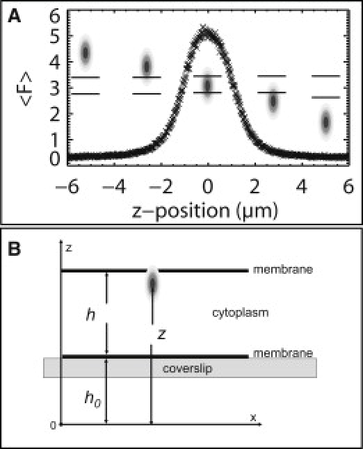
Z-scan approach to finite sample geometries of the living cell. (A) A COS cell containing EGFP was z-scanned through the cytoplasm. The average fluorescence intensity is plotted as a function of z position. The overlaid cartoon indicates the position of the excitation volume with respect to the cytoplasmic slab. A z scan acquires information for many z positions and provides an accurate description of the fluorescent signal from a thin sample which a single-point conventional FFS measurement cannot. (B) A cytoplasmic cell section is located at a height h₀ above the start of the z scan and has a thickness h. The position of the excitation light is described by the value of z.

We model each cytoplasmic section enclosed by the observation volume as a fluorescent slab. The diameter of a typical COS cell is ∼50 μm in the x-y plane with a thickness that decreases from the center (∼5 μm) to the periphery. The intensity of the excitation light is azimuthally symmetric. The axial direction is parallel to z, and the radial direction lies in the x-y plane (Fig. 2 B). Compared with the size of the cell along the x-y plane, the radial beam waist (∼0.5 μm) of the excitation light is small enough that the change in thickness of the cytoplasm section within the excitation light is negligible. Therefore, we model the cytoplasm section as a slab of constant height. The z scan begins well below the cell such that sample is first encountered at a height h₀. The cytoplasmic slab has a height h, and the position of the excitation light is described by the z coordinate of its center.

We now introduce the geometry function S(z) into FFS theory to account for a confined sample environment. For the specific example of a slab (Fig. 2 B) as described above, the function S(z) is given by

$$S\left(z;h_0,h\right)=\{\begin{array}{cc}1,& h_0<z<h_0+h\\ 0,& \text{otherwise}\end{array}.$$ (1)

The parameter h₀ is important for fitting experimental data, because it determines the difference between the start position of the scan and the start position of the slab. However, including the offset parameter h₀ into the theory development unnecessarily complicates the notation. We therefore set h₀ to zero and hereafter leave it out of the notation. It is straightforward to include the offset in the final equations by a linear transformation of z to z – h₀.

We define the volume of the point spread function (PSF) raised to the r^th power by

$$V_{{PSF}^r}\left(z\right)=\int {\text{PSF}}^r\left(\rho ,\zeta \right)·S\left(z+\zeta \right)d\Omega .$$ (2)

The variables ζ and ρ represent the local coordinates measured with respect to the center of the PSF. We explicitly make use of the cylindrical symmetry of the PSF with dΩ = 2πρ d ρ dζ. The position ζ in the local PSF-coordinate system translates to z + ζ in the experimental setup coordinate system. In addition, we adopt the convention that, in the absence of explicit integration limits, variables are integrated over all space.

This definition of $V_{PS{F}^r}\left(z\right)$ explicitly includes the geometry function S(z) to reflect that only part of the PSF is accessible to the fluorophore. The conventional FFS theory is recovered by choosing S(z) = 1, which corresponds to the infinite sample case, where the complete PSF is accessible. We explicitly refer to the infinite sample case by using the subscript ∞. Thus, V_∞,PSF is the volume of the PSF for the infinite case. The value of $V_{PS{F}^r}\left(z\right)$ for the restricted geometry depends on S(z) and the focus position z of the PSF. The fluorescence intensity F(t,z) of a solution of molecules with brightness λ confined in a finite sample is given by (1)

$$F\left(t,z\right)=\lambda \int PSF\left(\rho ,\zeta \right)·c\left(\rho ,\zeta ,t\right)·S\left(z+\zeta \right)d\Omega$$ (3)

with concentration c(ρ,ζ,t) at position (ρ,ζ) and at time t. The geometry function S(z) serves to restrict the sample size.

We now specifically consider the slab-geometry defined by Eq. 1. The PSF volume depends for this case on the height h, $V_{PS{F}^r}\left(z;h\right)$. For a stationary process, the average fluorescence and its variance is determined from Eq. 3 as

$$\langle F\left(z;h\right)\rangle =\lambda \langle c\rangle V_{PSF}\left(z;h\right),$$ (4)

and

$$\langle \Delta F^2\left(z;h\right)\rangle ={\lambda }^2·\langle c\rangle ·V_{PS{F}^2}\left(z;h\right)={\gamma }_2\left(z;h\right)·{\lambda }^2·\langle c\rangle ·V_{PSF}\left(z;h\right).$$ (5)

While the derivation of Eq. 4 is straightforward, Eq. 5 can be derived using the cumulants of the fluorescence (14) or by following the method used by Thompson (15). Equation 5 also introduces a geometry-dependent shape-factor

$${\gamma }_2\left(z;h\right)=\frac{V_{PS{F}^2}\left(z;h\right)}{V_{PSF}\left(z;h\right)},$$ (6)

which is a generalization of the conventional shape factor (15). All of the above equations are equivalent to the equations of conventional FFS, which are obtained by replacing $V_{PS{F}^r}$ by the value for the infinite sample case, $V_{\infty ,PS{F}^r}$.

Brightness and concentration are independent of geometry and thus are good parameters for characterizing the sample of interest. The mean fluorescence intensity 〈F〉 is an easily measured experimental quantity which is used to determine the size of the slab. Furthermore, we use Mandel's Q parameter (3,16)

$$Q\left(z;h\right)=\frac{\langle \Delta F^2\left(z;h\right)\rangle }{\langle F\left(z;h\right)\rangle }=g\left(0\right)·\langle F\rangle ={\gamma }_2\left(z;h\right)·\lambda ,$$ (7)

because it is a directly measurable quantity that relates to the brightness through the model-dependent shape factor γ₂. Q is determined by the ratio of the first two moments of the fluorescence intensity, or, alternatively, by the product of the fluctuation amplitude g(0) and the average fluorescence intensity as measured in an FCS experiment.

While we discussed the slab-model in the above section, it is straightforward to extend the model to other geometries by evaluating Eqs. 4–7 for other functions of S(z). Of particular interest is a sample thin enough that it resembles a layer with negligible thickness. We refer to this as a δ-layer sample, which has the corresponding shape-factor

$$S\left(z\right)=\delta \left(z\right).$$ (8)

The average fluorescence intensity for a δ-layer is

$$\langle F\left(z\right)\rangle =\lambda ·\langle \sigma \rangle ·{\text{RIPSF}}_1\left(z\right),$$ (9)

where 〈σ〉 is the area concentration of fluorophores within the δ-layer and RIPSF_r(z) defines the radially integrated PSF raised to the r^th power

$${\text{RIPSF}}_{\text{r}}\left(z\right)=\underset{0}{\overset{\infty }{\int }}{\text{PSF}}^r\left(\rho ,z\right)·2\pi \rho d\rho .$$ (10)

Thus, RIPSF₁(z) of Eq. 9 represents the radially integrated PSF, which we also refer to as RIPSF(z) in this article.

PSF model

The z-scan fluorescence intensity curve given by Eqs. 4 and 2 involves the convolution of the PSF and the sample geometry, as it is this overlap volume which generates the fluorescent signal. To model the convolution in a useful manner, it is first necessary to establish an accurate PSF of the experimental setup from fluorescence intensity curves. However, convolution of the PSF with the sample thickness obscures the features of the experimental PSF. To avoid this complication, we choose a δ-layer sample, which, according to Eq. 9, results in a fluorescence intensity curve that is directly proportional to the radially integrated PSF, RIPSF(z). This procedure directly evaluates the quality of a PSF-model in reproducing experimental data.

For this study, z scans are performed on a cytoplasmic section thin enough that it resembles a δ-layer. To identify a cytoplasmic δ-layer, we take a series of z scans across the cell moving toward increasingly thinner sections of the cytoplasm. While intensity z scans in the nucleus are broad, the width of the curve narrows as the cell height decreases. Below a certain thickness, the shape of the intensity z scan ceases to change. When this condition is met, we have reached an effective δ-layer.

FFS theory employs simple model functions in order to approximate the experimental PSF. In the following, the parameter n is used to account for the difference in the PSF for two-photon excitation (TPE) and one-photon excitation (OPE). We define the PSF models where n = 1 for OPE and n = 2 for TPE. Two PSF-models widely used are the three-dimensional Gaussian (3DG) PSF,

$$PS{F}_{3DG}\left(\rho ,\zeta \right)=\exp \left(-2n\left(\frac{{\rho }^2}{w_0^2}+\frac{{\zeta }^2}{z_0^2}\right)\right),$$ (11)

and the Gaussian-Lorentzian (GL) PSF,

$$PS{F}_{GL}\left(\rho ,\zeta \right)={\left(\frac{w_0}{w\left(\zeta \right)}\right)}^{2n}\exp \left(-2n\frac{{\rho }^2}{w^2\left(\zeta \right)}\right),$$ (12)

with

$$w\left(\zeta \right)=w_0{\left(1+\frac{{\zeta }^2}{z_0^2}\right)}^{\raisebox{1ex}{$1$}\!\left/ \!\raisebox{-1ex}{$2$}\right.}.$$ (13)

The radial and axial beam waists of the PSF are given by w₀ and z₀.While knowledge of the PSF is sufficient for TPE, the description of OPE is further complicated by the need to account for the effect of a pinhole on the collected fluorescence emission. This effect can be approximated by multiplying the excitation PSF by a collection profile function Ω(ρ,ζ) (15,17). Because our experimental work uses TPE, we analyze the experiments using a PSF-model with n = 2.

We now evaluate the suitability of these two model functions for z-scan FFS. It is straightforward to integrate each PSF over ρ to determine their RIPSF. Fig. 3 contains the intensity z scan of an effective δ-layer based on a very thin cytoplasmic section of a COS cell expressing EGFP. Fig. 3, A and B, display fits of the intensity curve to the RIPSF using the 3DG and GL model, respectively, plotted with a linear and logarithmic intensity axis to emphasize the tail of the radially integrated PSF. Simple visual inspection of the fits reveals that neither the 3DG nor GL model lead to a correct description of the experimental RIPSF.

Figure 3.

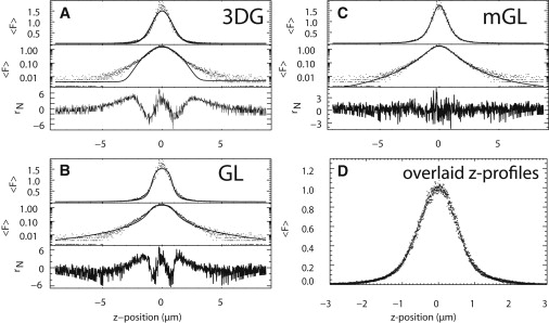
PSF models. A z-scan intensity trace is acquired from a thin section of cytoplasm in a cell containing EGFP. The same intensity trace is fit with three different point spread function (PSF) models. The intensity fits are plotted on a linear (upper panel) and semi-log scale (middle panel), along with the normalized residuals (lower panel). (A) The three-dimensional Gaussian model and (B) the Gaussian-Lorentzian model are two PSF models commonly used in conventional FFS, but do not accurately fit z-scan data. (C) We show that our modified Gaussian-Lorentzian (mGL) model permits the type of fit (i.e., more accurate) required for successful implementation of the z-scan technique. The mGL fit parameters for this data are z₀ = 1.1 ± 0.048 μm and y = 1.9 ± 0.056. (D) Z scans were performed across thin sections of five cells and normalized to a peak intensity of 1. The overlaid data demonstrate that the z-scan profile is stable and repeatable.

It is desirable to establish a PSF model that faithfully reproduces the z-scan intensity curves. Such a model is a prerequisite for employing a χ-square goodness-of-fit test to accept or reject the presence of protein interactions from brightness data. A far more sophisticated approach of modeling the PSF involves evaluating the electromagnetic-wave propagation through the microscope objective (17,18). However, such an approach requires extensive modeling and is numerically expensive. Ideally, we would like to establish a heuristic model function which has a simple analytical form and successfully reproduces the experimental data. Fig. 3 shows that both the 3DG and GL fits have strong correlations in their residuals. These correlations are typical for all cells scanned (not shown). Correspondingly, the reduced χ-squared values for 3DG and GL fits are consistently >4. Closer inspection of the fits reveals that the tail of the 3DG function decays too rapidly, while the tail of the GL function decays too slowly. This observation motivated the introduction of a modified Gaussian-Lorentzian (mGL) PSF,

$$PS{F}_{mGL}\left(\rho ,\zeta \right)={\left(\frac{w_0}{w\left(\zeta \right)}\right)}^{(1+y)n}\exp \left(-2n\frac{{\rho }^2}{w^2\left(\zeta \right)}\right).$$ (14)

The mGL-PSF contains the additional parameter y, which varies the exponent of the first factor of the GL-PSF. This heuristic model allows us to tune the steepness of the z decay of the PSF while maintaining a Gaussian cross section of the PSF. Note that for y = 1, the modified GL-PSF reduces to the original GL-PSF. The mGL-PSF successfully fits the experimental intensity curve (Fig. 3 C) with largely uncorrelated residuals and a reduced χ-square close to 1. The fit-parameters are z₀ ≈ 0.95 μm and y ≈ 1.9. Fig. 3 D shows overlaid z scans through very thin slices of five different cells. The peak intensities have been normalized to 1 to demonstrate that the RIPSFs all have the same shape and are reproducible. Thus, we will use the mGL-PSF for modeling of all further z-scan FFS experiments.

Z-scan fluorescence intensity curves of cells

We demonstrated that the mGL-PSF describes the z-scan intensity curve for a δ-layer geometry. Theoretically, we expect that knowing the radially integrated PSF is sufficient to describe any sample geometry S(z), because the volume of PSF′ is related to RIPSF via

$$V_{PS{F}^r}\left(z\right)=\int {\text{RIPSF}}_{\text{r}}\left(\zeta \right)·S\left(z+\zeta \right)d\zeta .$$ (15)

Thus, the z-scan fluorescence intensity curve may be written as

$$\langle F\left(z;h\right)\rangle =\lambda \langle c\rangle \int \text{RIPSF}\left(\zeta \right)·S\left(z+\zeta \right)d\zeta .$$ (16)

To test our prediction experimentally, multiple intensity z scans are taken at different positions in a single cell. Each cell position provides a different sample thickness, but brightness and concentration are expected to be identical within a given cell. Fig. 4 shows eight intensity z scans taken from a single cell expressing EGFP. The locations of the scans are roughly:

• 0, at the center of the nucleus,

• 1, next to the nuclear envelope at the nucleoplasmic side,

• 2, next to the nuclear envelope at the cytoplasmic side,

• 3–6, progressing radially outward through the cytoplasm, and

• 7, near the outer edge of the cell.

Figure 4.

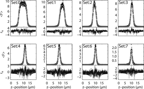
Intensity z scans fit with the mGL PSF model. Eight intensity z scans were taken in the same cell at different thicknesses. The locations are roughly: 0, at the center of the nucleus; 1, just inside the nuclear envelope; 2, just outside the nuclear envelope; 3–6, progressing radially outward through the cytoplasm; and 7, near the outer edge of the cell. All sections are fit using identical parameters for the modified GL PSF model, z₀ = 0.986 ± 0.009 μm and y = 2.000 ± 0.016. Thicknesses for cell sections 0–7 are 6.50, 4.03, 2.46, 2.02, 1.40, 1.18, 0.95, and 0.30 μm. The overall reduced χ-squared is 1.19.

Because EGFP is uniformly distributed in the cytoplasm and nucleus, all eight scans probe a geometry with a single fluorescent layer. The eight intensity z-scan experiments are simultaneously fit to a slab model with a variable thickness for each scan, but globally linked PSF-parameters z₀ and y.

The global fit resulted in a reduced χ-square of 1.2 with PSF-parameters z₀ = 0.986 ± 0.009 μm and y = 2.00 ± 0.016. The thicknesses for cell scans 0–7 are 6.50, 4.03, 2.46, 2.02, 1.40, 1.18, 0.95, and 0.30 μm. Note that samples thinner than ∼0.5 μm become effective δ-layers, and the slab model cannot accurately determine their thickness. The same experiment was repeated on other cells and on individual cell slices (data not shown) with similar results. The PSF parameters that best describe all z-scan experiments are z₀ = 0.95 ± 0.10 μm and y = 1.9 ± 0.14.

γ-Factor

We previously discussed that conventional FFS analysis leads to a spurious increase of the brightness of EGFP with decreasing sample thickness. This behavior is readily explained by considering Mandel's Q parameter, which in conventional FFS is related to the brightness by Q = γ_2,∞λ (3). Inspection of Eq. 7 illustrates that the failure of conventional FFS lies in assuming a γ-factor γ_2,∞ of an infinite sample, which neglects the actual geometry-dependence of the γ-factor γ₂(z;h). Thus, the brightness increase reflects the ratio of γ₂(z;h)/ γ_2,∞, which is 1 for a thick sample, but grows larger as the sample thickness decreases and reaches a limiting value as the thickness approaches a δ-layer. A suitable PSF-model needs to reproduce the experimentally observed change of γ₂(z;h)/ γ_2,∞ with thickness. Because γ₂ cannot be directly measured, we determine the Q parameter according to Eq. 7 from the first two fluorescence intensity moments. The ratio of the γ-factors is simply the ratio of the corresponding Q parameters,

$$\frac{{\gamma }_2\left(z;h\right)}{{\gamma }_{2,\infty }}=\frac{Q\left(z;h\right)}{Q_{\infty }}.$$ (17)

We measure this ratio of the Q parameter by taking FFS measurements in 10 cells expressing EGFP. Each cell is measured at various positions while focusing the beam at midheight on the cellular slab, which corresponds to z = h/2, where h is the height of the cellular slab. The experimental Q parameter, Q(h/2;h), is divided by Q_∞, which is obtained from a measurement in the nucleus or in bulk solution. The experimental ratio for Q parameters is identical to the experimental ratio of γ-factors that is plotted in Fig. 5 as a function of thickness h.

Figure 5.

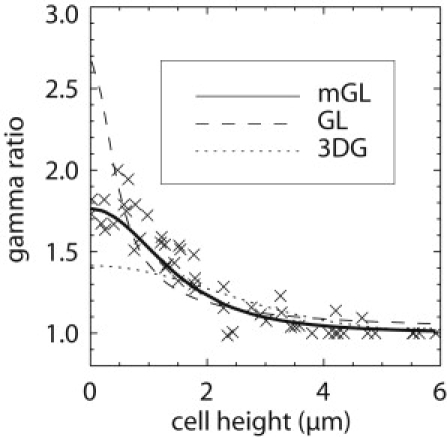
The γ-ratio: experiment and theory. The γ-ratio data is plotted for different positions in several cells containing EGFP. The γ-ratio is defined as γ₂(h/2;h) divided by γ_2,∞, where γ₂(h/2;h) is a geometry-dependent shape factor and γ_2,∞ is the infinite sample shape factor assumed by conventional FFS. Thick sample sections, like the nucleus, have an effectively infinite volume, and thus a γ-ratio equal to 1. The opposite limiting case, when the sample becomes a δ-layer, is sample-independent and thus a useful measure to test the PSF model we have developed. The traditionally chosen three-dimensional Gaussian and Gaussian-Lorentzian models do not fit the experimental data, especially in approach to the δ-layer limit. The mGL PSF model matches the behavior of experimental data.

Next we derive equations (Supporting Material) for the theoretical ratio γ₂(h/2;h)/γ_2,∞ using Eq. 6 as a function of thickness h for the GL-, the 3DG-, and the mGL-PSF and fit the expressions to the experimental data. The fits are shown together with the experimental γ-ratio in Fig. 5. Neither the 3DG- nor the GL-model fit the experiment. Only the mGL-PSF model reproduces the experimental data. The γ-factor ratio between a δ-layer and an infinite sample, γ₂(h/2;h)/γ_2,∞, provides a sensitive test of the PSF model because its value can be determined from the experimental data and compared to theory. The γ-ratios of the 3DG and GL models are $\sqrt{2}$ and 8/3, respectively, and the experimental value approaches ∼1.8 in the limit as h goes to 0. The mGL-model with z₀ ≈ 0.95 μm and y ≈ 1.9, on the other hand, yields a γ-factor ratio of 1.86, which is in close agreement with the experimental data. These results show that the mGL-PSF is successful in reproducing the experimental γ-factors for all different heights h of the sample.

Brightness by z-scan FFS

The experiments described so far indicate that the mGL-PSF provides an accurate description of the experimental PSF. We therefore expect to furnish unbiased brightness values from thin cell sections by analyzing FFS experiments with the mGL-model. The most straightforward approach to achieve an accurate brightness measurement from cell data requires an intensity z-scan measurement followed by an FFS measurement at the midsection of the cellular slab to determine the Q parameter. The intensity z scan provides the thickness h and axial-offset h₀ of the cellular slab, which is used to determine the γ-factor for the mGL-PSF at the midsection of the cell, γ_2,mGL(h/2;h). By using the proper γ-factor, the correct brightness λ is extracted from the Q parameter, Q = λ · γ_2,mGL(h/2;h). If the γ-factor γ_2,∞,GL for an infinite sample geometry is used instead, a biased brightness λ′ is recovered, Q = λ′γ_2,∞,GL. T.

The above strategy is now tested experimentally. We refer to the intensity z-scan followed by an FFS measurement at the midsection of the cell as z-scan FFS. We report brightness in normalized form, b = λ/λ_monomer, where λ_monomer is the brightness recovered for monomeric EGFP from a sample thick enough to avoid any bias in its brightness. For comparison we first show in Fig. 6 A the biased EGFP data (triangles) originally displayed in Fig. 1 B. The overestimation of the brightness with decreasing thickness of the sample is a consequence of conventional FFS analysis, which erroneously indicates the presence of dimeric EGFP in the cell.

Figure 6.

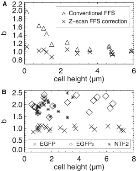
Z-scan corrected brightness analysis. (A) EGFP exists as a monomeric protein in cells (normalized brightness, b = 1), and distributes uniformly throughout the nucleus and cytoplasm. Data was taken at different locations in the cells, from the center of the nucleus out to the edge of the cell. Conventional FFS ignores sample thickness and yields biased results (triangles). Z-scan FFS corrects for sample geometry and recovers the unbiased brightnesses (crosses). The corrected normalized brightnesses show a value of 1, accurately reporting the existence of monomeric EGFP throughout the cell. (B) Additional experiments were conducted on cells containing the artificial dimer construct EGFP₂ (diamonds) and nuclear transport factor 2 (NTF2, asterisks). Z-scan corrected brightnesses are equal to 2 for NTF2 measured in high concentration cells (>1 μM), which indicates that NTF2 forms a homodimer in the cytoplasm of living cells.

We now determine the brightness of the same data using z-scan FFS. The fits of the z-scan intensity curves confirm that EGFP in the cell nucleus and cytoplasm is represented by a single, uniform layer that is accurately modeled by the mGL-PSF applied to a rectangular slab of height h (data not shown). The γ-factor γ_2,mGL(h/2;h) was determined from the z-scan intensity fit parameters and used to determine the brightness from the experimentally measured Q parameter. The recalculated brightness (crosses) is displayed in Fig. 6 A after accounting for the geometry-dependent γ-factor. As expected, the normalized brightness is 1 at all measured cell locations, meaning that EGFP is a monomer throughout the cell. This result provides strong evidence that z-scan experiments provide a successful method for the unbiased determination of brightness in the cytoplasm.

We repeated the z-scan FFS measurement on cells expressing the dimeric construct EGFP₂. Because EGFP₂ covalently links two EGFP molecules, a normalized brightness of 2 is expected from this artificial dimer. Z-scan FFS measurements are performed at five different positions in each cell measured. In addition, we performed z-scan FFS measurements on cells expressing EGFP as a control. The corrected brightness for each protein was determined by using the previously described method. Fig. 6 B plots the unbiased EGFP brightness (crosses) and the unbiased EGFP₂ brightness (diamonds) as controls. As expected, these normalized brightnesses are all ∼1 and ∼2, indicating monomers and dimers, respectively.

We now apply z-scan FFS to measure the oligomeric state of EGFP-labeled NTF2 in the cytoplasm of COS-1 cells. NTF2 plays an important role in maintaining the Ran-gradient, which is crucial for nucleocytoplasmic transport (19). In vitro data report that NTF2 exists as a dimer at concentrations exceeding 1 μM (20), but a direct confirmation of the dimeric state of NTF2 in cells is not yet available. We therefore performed cytoplasmic z-scan FFS experiments on EGFP-NTF2 at concentration exceeding 1 μM and demonstrate that the brightness (asterisks) falls on top of the EGFP₂ data, showing that NTF2 is a dimer (Fig. 6 B). Conventional FFS analysis of the data would lead to a large scatter of brightness values with an average that exceeds the value expected for a dimer. This behavior complicates proper identification of the degree of oligomerization, which is avoided by using z-scan FFS.

Discussion

This study demonstrates that once the sample thickness approaches the axial dimension of the optical observation volume, the brightness determined by conventional FFS experiences a sample thickness-dependent bias. The degree of bias depends on the optical setup and the cell type studied. Spreading cells typically have a thickness of a few micrometers at the center, which drops with distance from the center. The axial beam waist of the excitation light depends on the optical setup, but is typically ∼1 to a few micrometers. Thus, the potential for brightness bias in cell experiments is a concern. Because the cell is usually thickest at the center, the likelihood of brightness artifacts increases for cell measurements taken at off-center positions.

We define the thickness which leads to a 20% bias in brightness as critical thickness. The critical thickness depends on the instrument and needs to be evaluated on an individual basis. Our instrumental setup leads to a critical thickness of 2 μm. We reported thicknesses of COS-1 cells in the cytoplasm of ∼2.5 μm to <1 μm. Thus, we observe brightness bias in cytoplasmic FFS measurements. Only measurements conducted directly next to the nuclear envelope on the cytoplasmic side of COS-1 cells are generally thick enough to avoid significant brightness bias. However, this location contains the endoplasmic reticulum and Golgi complex. If these organelles need to be avoided experimentally, measurements have to be taken further away from the nuclear envelope, where the thickness falls below the critical value. For example, the phosphatidylinositol type II kinase (P14KII) interacts with endosomal membranes (21), which prevent the quantitative FFS measurement of cytoplasmic P14KII next to the nuclear envelope. Thus, cytoplasmic P14KII has to be measured further away from the nucleus, where brightness corrections are important.

The cell line used in the experiments is another important factor. We have found that CV-1 cells exhibit a shallower height profile than COS-1 cells. Thus, cytoplasmic FFS measurements in CV-1 cells are at the critical thickness even when conducted directly next to the nuclear envelope. It is also important to recognize that while a cell population has a typical height profile, cell-to-cell variations exist. Thus, the same relative location may be above or below the critical thickness in different cells.

The excitation beam profile is the chief factor in determining the critical thickness. The long axial tail of the GL-PSF makes it especially prone to thickness artifacts, which is an important consideration for two-photon excitation experiments. For example, a GL-PSF with an axial beam waist of 1 μm leads to a critical thickness of 5 μm. Because the thickness of COS-1 cells at the center is ∼5 μm, a GL-PSF would introduce a brightness bias for all cell measurements. Thus, underfilling the back aperture of the objective, which leads to a GL beam profile, should be avoided when performing cell measurements. Because the optics of each instrument differ and the presence of aberrations influences the PSF, it is necessary to characterize the critical thickness of each instrument separately.

The presence of brightness bias is not necessarily easy to recognize. It becomes apparent when graphing the brightness versus thickness as shown in Fig. 1 B, but typical FFS experiments do not record this information. Because FFS studies in cells require the measurement of a large number of cells to acquire sufficient statistics, the variations of thickness of the sample simply increase the scatter of the measured brightness values. Because the bias always results in larger brightness values, the interpretation of the data are systematically skewed toward identifying stronger protein interactions than actually exist. For example, in a system where protein-protein interactions are absent, the bias results in a normalized brightness exceeding 1. This leads to the erroneous conclusion that the proteins do interact. Similarly, quantitative interpretation of binding curves and protein stoichiometries from brightness titration data is also compromised. Brightness corrections are especially important for FFS measurements of proteins at the periphery of the cell, such as would be required in the case of focal adhesion studies. A similar example is FFS in bacteria, such as Escherichia coli, which have a diameter smaller than the critical thickness. In addition to FFS measurements at a single location, brightness measurements using imaging approaches (22) are susceptible to the same artifact.

To perform quantitative brightness experiments in thin environments, it is necessary to address the brightness bias. The problem is solved by performing a fluorescence intensity z scan before the FFS measurement to characterize the thickness and correct the FFS analysis. It only takes ∼5 s to execute the intensity z scan, which is short compared to the FFS data acquisition time (∼60 s). Thus, the additional measurement time for carrying out z-scan FFS is negligible. Z-scan FFS only requires a motorized microscope stage and is straightforward to implement. Z-scan FFS experiments should be carried out with a water-immersion instead of an oil-immersion objective, because spherical aberrations need to be minimized.

We applied z-scan FFS to investigate the oligomeric state of NTF2 in the cytoplasm. Biochemical studies and an ultracentrifugation experiment report that NTF2 forms a dimer (20,23). Our work confirms that NTF2 exists as a dimer in the cytoplasm of living cells. NTF2 is also known to interact with nucleoporin proteins at the nuclear envelope (19,24), which leads to nuclear rim staining. As a consequence, the fluorescence intensity at the nuclear envelope is enhanced, which prevents us from measuring the brightness of NTF2 in the nucleus. We performed cytoplasmic FFS measurements away from the nuclear envelope to avoid signal contributions from nuclear rim staining. Therefore, all these measurements had to be corrected for the finite thickness of the sample.

NTF2 interacts with the nuclear pore complex and mediates active transport across the pore by an unknown mechanism. We are interested in extending z-scan FFS in the future to measure protein interactions and transport rates directly at the nuclear membrane to investigate the transport process. This will require an expansion of z-scan FFS to a multilayer geometry and should open up a number of interesting applications of the technique to the study of internal membrane interfaces.

A multilayer sample can no longer be characterized by a single FFS measurement at the midsection as performed in this article. A natural extension of this work takes several FFS measurements as a function of the z position. The geometry function S(z) is easily modified to describe multiple layers, and z-scan FFS can be implemented for complex samples, only being limited by the resolvability of the layers through a fit to the model. Thus, z-scan FFS should be able to make direct measurements of brightness at internal membrane interfaces like the nuclear envelope; these regions have been previously inaccessible to quantitative brightness analysis.

Z-scan methods have been previously implemented into FFS to study diffusion in membranes such as giant unilamellar vesicles and supported phospholipids bilayers (11,12). These studies were performed in isolated membrane systems, but related z-positioning FCS techniques are now being used to study raft diffusion properties in the plasma membrane of living cells (13,25). Here, we extend the use of z-scanning to study the brightness in thin sample geometries. Although this work focuses mainly on cell measurements, the same problem of brightness bias is encountered in micrometer and submicrometer fluidic devices. Thus, z-scan FFS has potential applications in thin microfluidic channels.

While thin sample geometry limits the access of fluorophores to the excitation light, it also limits the possible movement of the particles. As the sample flattens out, diffusion of proteins is no longer accurately described by a three-dimensional diffusion model. Gennerich and Schild (26) deal extensively with the effect that confined geometry has on diffusion, as calculated by FCS. Fortunately, brightness is independent of diffusion time, provided that no undersampling occurs (27). All FFS measurements in this study were sampled sufficiently quickly to avoid any undersampling. If necessary, brightness values may be corrected for undersampling effects as previously described (27).

In summary, this article describes a sample thickness-dependent artifact of FFS data which leads to an increase in brightness. We report a brightness bias of cytoplasmic FFS measurements in COS-1 cells, which in the worst case leads to an approximate doubling of the brightness value. Because brightness analysis is frequently used to detect protein association, a factor-of-2 bias is a critical problem for quantitative measurements.

This article describes how the critical thickness is identified and provides advice on performing FFS measurements in the cytoplasm of cells. We introduced z-scan FFS as a simple method to assess the thickness of the sample and provide brightness values free of artifact. Z-scan FFS provides a general method for brightness determination in cases where the finite thickness of the sample is of concern. We expect that z-scan FFS should prove especially useful for FFS applications in the cytoplasm and other thin geometries.

References

- 1.Elson E.L., Madge D. Fluorescence correlation spectroscopy. I. Conceptual basis and theory. Biopolymers. 1974;13:1–27. doi: 10.1002/bip.1974.360130103. [DOI] [PubMed] [Google Scholar]
- 2.Rigler R., Mets U., Kask P. Fluorescence correlation spectroscopy with high count rate and low background: analysis of translational diffusion. Eur. Biophys. J. 1993;22:169–175. [Google Scholar]
- 3.Chen Y., Mueller J.D., Gratton E. The photon counting histogram in fluorescence fluctuation spectroscopy. Biophys. J. 1999;77:553–567. doi: 10.1016/S0006-3495(99)76912-2. [DOI] [PMC free article] [PubMed] [Google Scholar]
- 4.Kask P., Palo K., Gall K. Fluorescence-intensity distribution analysis and its application in biomolecular detection technology. Proc. Natl. Acad. Sci. USA. 1999;96:13756–13761. doi: 10.1073/pnas.96.24.13756. [DOI] [PMC free article] [PubMed] [Google Scholar]
- 5.Petersen N.O., Hoddelius P.L., Magnusson K.E. Quantitation of membrane receptor distributions by image correlation spectroscopy: concept and application. Biophys. J. 1993;65:1135–1146. doi: 10.1016/S0006-3495(93)81173-1. [DOI] [PMC free article] [PubMed] [Google Scholar]
- 6.Qian H., Elson E.L. On the analysis of high order moments of fluorescence fluctuations. Biophys. J. 1990;57:375–380. doi: 10.1016/S0006-3495(90)82539-X. [DOI] [PMC free article] [PubMed] [Google Scholar]
- 7.Palmer A.G., Thompson N.L. High-order fluorescence fluctuation analysis of model protein clusters. Proc. Natl. Acad. Sci. USA. 1989;86:6148–6152. doi: 10.1073/pnas.86.16.6148. [DOI] [PMC free article] [PubMed] [Google Scholar]
- 8.Chen Y., Wei L.N., Mueller J.D. Probing protein oligomerization in living cells with fluorescence fluctuation spectroscopy. Proc. Natl. Acad. Sci. USA. 2003;100:15492–15497. doi: 10.1073/pnas.2533045100. [DOI] [PMC free article] [PubMed] [Google Scholar]
- 9.Chen Y., Tekmen M., Wu B. Dual-color photon-counting histogram. Biophys. J. 2005;88:2177–2192. doi: 10.1529/biophysj.104.048413. [DOI] [PMC free article] [PubMed] [Google Scholar]
- 10.Wu B., Chen Y., Mueller J.D. Heterospecies partition analysis reveals binding curve and stoichiometry of protein interactions in living cells. Proc. Natl. Acad. Sci. USA. 2010;107:4117–4122. doi: 10.1073/pnas.0905670107. [DOI] [PMC free article] [PubMed] [Google Scholar]
- 11.Korlach J., Schwille P., Feigenson G.W. Characterization of lipid bilayer phases by confocal microscopy and fluorescence correlation spectroscopy. Proc. Natl. Acad. Sci. USA. 1999;96:8461–8466. doi: 10.1073/pnas.96.15.8461. [DOI] [PMC free article] [PubMed] [Google Scholar]
- 12.Benda A., Beneš M., Hof M. How to determine diffusion coefficients in planar phospholipid systems by confocal fluorescence correlation spectroscopy. Langmuir. 2003;19:4120–4126. [Google Scholar]
- 13.Humpolíčková J., Gielen E., Engelborghs Y. Probing diffusion laws within cellular membranes by Z-scan fluorescence correlation spectroscopy. Biophys. J. 2006;91:L23–L25. doi: 10.1529/biophysj.106.089474. [DOI] [PMC free article] [PubMed] [Google Scholar]
- 14.Wu B., Mueller J.D. Time-integrated fluorescence cumulant analysis in fluorescence fluctuation spectroscopy. Biophys. J. 2005;89:2721–2735. doi: 10.1529/biophysj.105.063685. [DOI] [PMC free article] [PubMed] [Google Scholar]
- 15.Thompson N.L. Fluorescence correlation spectroscopy. In: Lakowicz J.R., editor. Vol. 1. Plenum Press; New York: 1991. (Topics in Fluorescence Spectroscopy). [Google Scholar]
- 16.Mandel L. Sub-Poissonian photon statistics in resonance fluorescence. Opt. Lett. 1979;4:205–207. doi: 10.1364/ol.4.000205. [DOI] [PubMed] [Google Scholar]
- 17.Hess S.T., Webb W.W. Focal volume optics and experimental artifacts in confocal fluorescence correlation spectroscopy. Biophys. J. 2002;83:2300–2317. doi: 10.1016/S0006-3495(02)73990-8. [DOI] [PMC free article] [PubMed] [Google Scholar]
- 18.Gregor I., Enderlein J. Focusing astigmatic Gaussian beams through optical systems with a high numerical aperture. Opt. Lett. 2005;30:2527–2529. doi: 10.1364/ol.30.002527. [DOI] [PubMed] [Google Scholar]
- 19.Bayliss R., Ribbeck K., Stewart M. Interaction between NTF2 and xFxFG-containing nucleoporins is required to mediate nuclear import of RanGDP. J. Mol. Biol. 1999;293:579–593. doi: 10.1006/jmbi.1999.3166. [DOI] [PubMed] [Google Scholar]
- 20.Chaillan-Huntington C., Butler P.J.G., Stewart M. NTF2 monomer-dimer equilibrium. J. Mol. Biol. 2001;314:465–477. doi: 10.1006/jmbi.2001.5136. [DOI] [PubMed] [Google Scholar]
- 21.Balla A., Tuymetova G., Balla T. Characterization of type II phosphatidylinositol 4-kinase isoforms reveals association of the enzymes with endosomal vesicular compartments. J. Biol. Chem. 2002;277:20041–20050. doi: 10.1074/jbc.M111807200. [DOI] [PubMed] [Google Scholar]
- 22.Digman M.A., Dalal R., Gratton E. Mapping the number of molecules and brightness in the laser scanning microscope. Biophys. J. 2008;94:2320–2332. doi: 10.1529/biophysj.107.114645. [DOI] [PMC free article] [PubMed] [Google Scholar]
- 23.Corbett A.H., Silver P.A. The NTF2 gene encodes an essential, highly conserved protein that functions in nuclear transport in vivo. J. Biol. Chem. 1996;271:18477–18484. doi: 10.1074/jbc.271.31.18477. [DOI] [PubMed] [Google Scholar]
- 24.Lane C.M., Cushman I., Moore M.S. Selective disruption of nuclear import by a functional mutant nuclear transport carrier. J. Cell Biol. 2000;151:321–332. doi: 10.1083/jcb.151.2.321. [DOI] [PMC free article] [PubMed] [Google Scholar]
- 25.Bacia K., Scherfeld D., Schwille P. Fluorescence correlation spectroscopy relates rafts in model and native membranes. Biophys. J. 2004;87:1034–1043. doi: 10.1529/biophysj.104.040519. [DOI] [PMC free article] [PubMed] [Google Scholar]
- 26.Gennerich A., Schild D. Fluorescence correlation spectroscopy in small cytosolic compartments depends critically on the diffusion model used. Biophys. J. 2000;79:3294–3306. doi: 10.1016/S0006-3495(00)76561-1. [DOI] [PMC free article] [PubMed] [Google Scholar]
- 27.Mueller J.D. Cumulant analysis in fluorescence fluctuation spectroscopy. Biophys. J. 2004;86:3981–3992. doi: 10.1529/biophysj.103.037887. [DOI] [PMC free article] [PubMed] [Google Scholar]
Associated Data
This section collects any data citations, data availability statements, or supplementary materials included in this article.