

Abstract
Eukaryotic cell crawling is a highly complex biophysical and biochemical process, where deformation and motion of a cell are driven by internal, biochemical regulation of a poroelastic cytoskeleton. One challenge to building quantitative models that describe crawling cells is solving the reaction-diffusion-advection dynamics for the biochemical and cytoskeletal components of the cell inside its moving and deforming geometry. Here we develop an algorithm that uses the level set method to move the cell boundary and uses information stored in the distance map to construct a finite volume representation of the cell. Our method preserves Cartesian connectivity of nodes in the finite volume representation while resolving the distorted cell geometry. Derivatives approximated using a Taylor series expansion at finite volume interfaces lead to second order accuracy even on highly distorted quadrilateral elements. A modified, Laplacian-based interpolation scheme is developed that conserves mass while interpolating values onto nodes that join the cell interior as the boundary moves. An implicit time-stepping algorithm is used to maintain stability. We use the algoirthm to simulate two simple models for cellular crawling. The first model uses depolymerization of the cytoskeleton to drive cell motility and suggests that the shape of a steady crawling cell is strongly dependent on the adhesion between the cell and the substrate. In the second model, we use a model for chemical signalling during chemotaxis to determine the shape of a crawling cell in a constant gradient and to show cellular response upon gradient reversal.
Keywords: diffusion, moving boundaries, numeric method, level set
1 Introduction
Moving boundary problems are notoriously difficult. Even for linear, dynamical equations, the presence of a free or otherwise mobile boundary can add sufficient complexity to make analytic solutions onerous or impossible. Therefore, computational methods are often necessary. Even then, the ability to accurately track the boundary and solve the bulk physical or chemical equations numerically is challenging. A classical example of this is the Stefan problem that examines heat flux in a material that can undergo termperature-induced phase changes. This long-standing problem is still actively researched using both analytical and numerical techniques [1–5].
Modeling cell motility is even more difficult. Many eukaryotic cells can move when in contact with a surface, the extracellular matrix, or other cells. This process is known as cell crawling and plays a significant role in developmental biology, cancer metastasis, and wound healing. In most eukaryotic cells, the primary structural component is the cytoskeleton, which is composed of actin filaments and microtubules. Crawling motility typically relies on the actin network and has been shown to entail three major biophysical processes: protrusion of the actin network at the front of the cell, adhesion to the surface, and pulling forward of the rear of the cell [6,7]. A description of the process by which cells achieve this motility is as follows. Chemical signals from outside the cell activate membrane bound proteins, which act to activate or enhance local actin polymerization [8,9]. Actin polymerization pushes out the front of the cell, most likely driven by a process known as the polymerization ratchet [10]. Once polymerized, the biochemical processes that modify and/or depolymerize the actin network are quite complex [11]. Focal adhesions are highly regulated assemblies of a large number of different molecules that form at the front of the cell and then mature as they move rearward with the actin network [12]. These adhesions provide anchorage of the cell to the external environment. The mechanism whereby cells pull up the rear is often attributed to an actomyosin contraction [13], but other groups have also suggested that depolymerization of the network may play a role [14,15]. Therefore, a complete model for cell motility needs to evolve a complex biochemical kinetic system that drives internal force production and leads to boundary displacement. As the cell membrane prevents many of the chemical species from leaving the cell, a method that can conserve the total mass of each species is preferred.
Many models for cell motility have focused on steady crawling, where the geometry of the cell is assumed to remain fixed as the cell crawls forward, thereby ignoring the moving boundary problem [15–18]. Recently, the level set method has been used in order to simulate the biochemical reactions inside a cell moving with prescribed boundary conditions [19], and others have used finite element methods to explore the mechanical deformations in a migrating cell [20–22] or the Pott’s model to simulate cell motility driven by chemical reactions [23]. Here we develop the Moving Boundary Node method: a general method for handling moving boundary problems with internal physical and/or chemical constituents that can be used to define the boundary velocity. In Sec. 2, we describe our method. In Sec. 3, we construct a number of test cases to determine the accuracy of the method. We show that the algorithm accurately solves reaction-diffusion-advection problems in 2D and also can be used for 2D surfaces embedded in 3D. We then apply this algorithm to simple models for cell crawling. As the algorithm presented here is not the only method that can handle free boundary problems, in Sec. 4 we compare the Moving Boundary Node Method to existing numerical methods. The final section is the conclusion, which summarizes our method with particular attention to biological applications.
2 Numerical Method
The algorithm that we develop here is a composite algorithm that separates boundary motion from the solution of the internal chemistry/physics. We focus on problems in two dimensions, but the methods that we develop are extendable to three dimensions.
We use a standard implementation of the Level Set method to move the boundary [30]. This method defines a signed distance map on a Cartesian grid and evolves it in time. The zeros of this function provide sub-pixel resolution of the boundary. Using the information stored in the distance map, we construct a resolved finite volume discretization of the geometry that is second order in space, while, topologically, grid nodes retain simple Cartesian connectivity. To evolve the system in time, we construct a discretization of the geometry at time t and at time t+ Δt. Then, using a modified Crank-Nicolson-type scheme that takes into account the change in the volumes between the two time steps, we evolve the contents of each finite volume. A Laplacian-based interpolation scheme is constructed that sets values on new nodes and globally conserves mass. We also describe a method for defining internal flow inside the geometry, which provides an advection velocity that can be used to transport internal chemical components.
The basic flow of our algorithm is as follows:
Define initial conditions for the distance map and internal chemical/physical components.
Mask for nodes that are inside the current geometry and interpolate onto newly uncovered nodes, if needed.
Construct a finite volume discretization of the derivative terms for the current geometry.
Calculate the boundary velocity.
Displace the boundary using the Level Set algorithm.
Using the same masked nodes, compute a new finite volume discretization of the derivative terms for the new geometry.
Use a semi-implicit method to evolve the contents of each finite volume.
Repeat steps (2) – (7) for each time step.
For linear dynamic equations, steps (2) – (7) represent a full time step evolution of the dynamics. For nonlinear problems, we propose using a second-order Runge-Kutta method, based primarily on the midpoint rule, as is used in Immersed Boundary methods [24]. For these problems, each time step involves a preliminary substep to the half-time level followed by a final substep from time t to time t + Δt, and steps (2) – (7) represent the procedure that is used for each substep. The specific details for how these steps are handled are discussed in the following subsections.
2.1 Level Set method
The Level Set method is a robust, general method for numerically tracking boundary movements [25–28]. Level set methods use a continuous function, ψ ∈ ℝn, to describe a boundary in ℝn−1. The common choice for ψ is the signed distance map, which is the distance of any point in space to the nearest point on the boundary, where negative values correspond to points inside the boundary. The position of the boundary is defined by the zero level set,
| (1) |
and the normal direction to any contour of ψ is
| (2) |
Motion of the boundary evolves via an advection equation,
| (3) |
where V is a velocity that is defined at all points in space. For many applications, V is only known at the boundary, in which case an extension velocity with the correct limit as ψ → 0 must be computed for all distant points.
2.1.1 Calculation of the extension velocity
We assume that the value of V at the boundary is given by the internal biochemistry and physics and that it points along the normal direction, V = V N̂. To extrapolate this velocity to each point inside the computational domain, we use a modified version of the extension velocity algorithm [29], which uses the orthogonality criterion,
| (4) |
to define V.
Following [31], we solve Eq. 4 inside a band of points about the zero contour. The narrow band is defined by |ψ| < 5h, where h is the grid spacing. We developed an implicit solver to integrate (4) inside this band. We consider N̂·∇ to be a matrix operator that can be broken up into two pieces, NxDx + Ny Dy, where Nx and Ny are the x and y components of N̂, and Dx and Dy are discrete versions of the x and y derivative operators, respectively.
To construct the matrix that corresponds to NxDx ψ, we first mask for all points in the domain that are inside the narrow band and have ψ Nx < 0. For all nodes inside this mask, if the node at (i, j) has neighbors (i+1, j), (i+2, j), and (i + 3, j) that are also inside the narrow band, then we construct the third order accurate approximation to the purely upwind, first derivative,
| (5) |
If the neighbors at (i + 1, j) and (i + 2, j) are inside the narrow band, but (i + 3, j) is outside, then we use the second order accurate, upwind derivative,
| (6) |
and, if only (i + 1, j) is inside the narrow band, then we use the first order accurate, upwind derivative,
| (7) |
For all points in the narrow band that have ψ Nx ≥ 0 and have neighbors (i − 1, j), (i − 2, j), and (i − 3, j) that are inside the narrow band,
| (8) |
If the neighbors at (i − 1, j) and (i − 2, j) are inside the narrow band, but (i − 3, j) is outside, then
| (9) |
and, if only (i − 1, j) is inside the narrow band, then
| (10) |
A similar discretization handles the y components and is easily generalizable to three dimensions. For smooth geometries, this method can provide up to fourth order accuracy (results not shown).
Standard methods such as Gauss-Jordan elimination or conjugate gradient methods can then be used to implicitly solve the linear system that corresponds to Eq. 4 inside the narrow band. For the simulations in this paper, we coded our routines in MATLAB and used the backslash function to invert this system of equations.
For points outside the narrow band we use the interpolation scheme described in [31] to define values of V that satisfy Eq. 4. This alogrithm determines the value of V (xi,j ) by interpolating the velocity field at the point xi,j − (ψN̂)i,j; i.e, points outside the band can be determined completely in terms of points that fall inside the narrow band. In this paper, we use cubic interpolation.
2.1.2 Time evolution of the distance map
At the start of each time step, we test the quality of the distance map. We do this by calculating the magnitude of the gradient of ψ inside a band of width 6h about the zero contour. The derivatives are calculated using a WENO discretization [28,30]. If |∇ψ − 1| > 0.01, then we reinitialize the distance map using the method described in [30].
We then solve Eq. 3 on a periodic, Cartesian domain. Spatial-discretization is handled using WENO derivatives, and a third order TVD Runge-Kutta method is used for time-stepping [30].
2.2 Finite volume discretization
In this section, we describe our method for constructing a finite volume discretization of the irregular geometry that is defined by the zero contour of a signed distance map. As mentioned previously, we work with a distance map that is defined on a M × N Cartesian grid. Our method distorts a Cartesian grid, while maintaining node connectivity, to yeild a node-centered finite volume representation with boundary-fitted control volumes. We then construct operators that define the first derivatives and the generalized diffusion operator on this irregular geometry.
2.2.1 Grid distortion
The signed distance map describes the distance from any point in space to the nearest point on the boundary; i.e., the nearest point on the boundary from the grid position xi,j can be defined as
| (11) |
We consider the nodes of the Cartesian grid as identifying quadrilateral areas. A quadrilateral is considered to be inside the geometry if interpolation gives a value of ψ less than zero at the center of a quadrilateral (Figure 1a). Boundary nodes are nodes with at least one neighboring grid point outside the boundary (open circles in Figure 1a) Boundary quads are then quadrilaterals which have at least one boundary node as a corner (red x’s in Figure 1a). With this scheme, it is possible to get boundary nodes that are only connected to exterior or boundary nodes. These nodes represent unresolved features and are removed from the mask of interior points. The remaining boundary nodes are then displaced using Eq. 11, thereby constructing a discrete representation of the geometry (Figure 1b).
Fig. 1.

Construction of the finite volume discretization. (a) Grid boxes with centers inside the boundary are identified; i.e., the value of ψ interpolated onto the center of the quads is less than zero (quads shaded in blue). The edge quads (red x’s) and the nodes that lie near the boundary (open circles) are identified. These boundary nodes are displaced a distance − ψ along the normal direction (arrows). (b). Displacement of grid nodes replaces grid boxes with quadrilaterals that fit the boundary. Blue shaded quads are inside the geometry and the nodes are shown as black dots.
A nice feature of this representation is that each node in the irregular geometry refers to a node located on the Cartesian grid. Therefore, the connectivity of the nodes is given. In addition, the resolved boundary removes the necessity of using ghost point methods, as has been used with other Level Set based algorithms [30]. However, moving the boundary nodes with Eq. 11 can lead to large deformations of the rectangular grid, which can produce inaccuracies when standard finite volume methods are employed [32]. To overcome this difficulty, we have developed a quad-based discretization that maintains second order accuracy even when the quads become greatly deformed.
We consider the quad shown in Figure 2a that is defined by nodes 1, 2, 3, and 4. The center of the quad is defined using the center of mass,
Fig. 2.

(a). A distorted quadrilateral area defined by the nodes labeled 1 – 4. The center of the quad is denoted by ⊗ and is labeled as location 5. We focus our attention on the node labeled 1. The subcontrol volume about this point, Δv1, is shaded in grey. The text describes computation of the flux through the eastern side of the area, which is centered about the point labeled 0. The normal vector along this side is n̂. (b). Schematic showing the full control volume about node 1, ΔV1 (shaded in grey), which is subdivided into three subcontrol volumes. (Note that here node 1 is a boundary node. Interior nodes have four control volumes.) To compute the total number of particles entering the control volume of node 1 in a unit time, we integrate the flux over the boundary of ΔV1. Volume integration is achieved by integrating over each subcontrol volume and then summing.
| (12) |
Focusing on node 1, we define a subcontrol volume about this node, Δv1, using the node, x1; the point that bisects the line between nodes 1 and 2, (x1 + x2)/2; the quad center, x5; and the point that bisects the line between nodes 1 and 4, (x1 + x4)/2. By breaking this subcontrol volume into two triangles and using the standard formula for the area of a triangle, we find the area for this subcontrol volume,
| (13) |
Note that this subcontrol volume is not necessarily the total control volume for node 1, as node 1 may also be connected to other quadrilaterals that will contribute to the total control volume (Fig. 2b). We distinguish between the total control volume and the subcontrol volume about node 1 by ΔV1 and Δv1, respectively.
2.2.2 Volume integration operators
In a finite volume discretization, it is necessary to compute the integrals of quantities, such as chemical concentrations, over the control volumes [32]. The standard way of handling this integration is to multiply the value of the concentration at the node by the control volume. For nodes that reside on or near the boundary, however, the node is not necessarily located at the center of its control volume, and therefore does not represent the average value of the concentration within the control volume. The extreme cases are the boundary nodes that reside on the edge of their control volume. Using the node values to represent the average value of the concentration inside the volume can introduce a small amount of error and can also lead to changes in the total mass during time stepping.
In place of the standard method, we choose to approximate the integral over each subcontrol volume. Summing the integrals over all the subcontrol volumes about each node then provides an approximation to the integral over the full control volume. Since each of the subcontrol volumes are centered about a non-grid point (See Fig. 2), we use bilinear interpolation to describe the concentration at the centers of the subcontrol volumes. In terms of the shaded subcontrol volume depicted in Fig. 2b, we define the integral of a function f over this shaded region to be
| (14) |
where the bar represents that the quantity is the integral of the function over the subcontrol volume. Therefore, the integral of a function over the total control volume about the ith node is
| (15) |
The subscript Δvi on the sum denotes that the sum is over the subcontrol volumes for the ith node. Eq. 14 couples nearby nodes, and, therefore, the integral over the total control volume (Eq. 15) also couples nearby nodes. We define a matrix  that computes this integral over control volumes given the vector of values of a function f defined on the nodes,
| (16) |
2.2.3 First derivative opeartors
To compute the finite volume approximation to the first derivatives of a function f, we use the identity
| (17) |
where S is the surface enclosing the volume V and n̂ is the outward directed normal to the volume. This identity can be broken into components, leading to
| (18) |
where ΔVi,j is the total control volume about the node located at xi,j.
To calculate the contribution to these derivatives at node 1 that comes from the control volume edge that separates the subcontrol volume about node 1 from that about node 2 in Figure 2a, we use bilinear interpolation to define the value of f at the quadrilateral center,
| (19) |
Then, the value of f at the center of the control volume edge can be approximated as
| (20) |
and the contributions to the derivatives from this edge are
| (21) |
| (22) |
where is the length of this edge of the control volume ΔV1. These contributions are equal to the contribution to the derivatives at node 2 along this same edge. All control volume edges that lie inside the quadrilaterals are defined in a similar fashion.
If a node in the quadrilateral is a boundary node, then we need to calculate the contributions from the boundary edges separately. Consider that the edge between node 1 and 4 is a boundary edge (as is shown in Fig. 2b). For this case, the contributions to the derivatives at node 1 from the control volume edge defined by the line between nodes 1 and 4 are
| (23) |
| (24) |
where x̂ and ŷ are unit vectors in the x and y directions, respectively. We denote the matrix operators that correponds to these discretizations as  and
and  , such that
| (25) |
| (26) |
Here the sum is over all of the control volume faces, and the approximate equivalence reflects that these matrices give approximations to the derivatives.
2.2.4 First derivatives related to transport
For equations that have first order spatial derivatives related to transport, such as would come from a continuity equation, i.e., terms of the form ∇ · (f v), we compute ∂(f vx)/∂x and ∂(f vy )/∂y using the same method that was described in the previous section for calculating the gradient. Specifically, we use that the contribution to the derivatives at node 1 from the control volume edge between node 1 and 2 in Figure 2a is given by
| (27) |
| (28) |
where
| (29) |
| (30) |
As before, the total contribution to these derivatives is computed by summing over all faces of the control volumes. We denote the matrices that correpond to the integrals over the control volume of Eqs. 27 – 28 as  (vx) and
  (vy), which are shown here with explicit dependence on the components of the velocity.
2.2.5 Generalized diffusion operator
To construct a scheme that can handle general descriptions of biochemistry and physics inside moving geometries may require the solution to diffusion-like equations that have spatially-dependent diffusion coefficients. Furthermore, if the cytoskeleton behaves like an elastic solid then a physical description of the cytoskeleton may also require an effective diffusion coefficient that depends on direction. Indeed, recent experiments show that the elastic behavior of the cytoskeleton of crawling nematode sperm behaves anisotropically [15]. Therefore, we seek a discretization for terms of the form
| (31) |
where νx and νy are spatially-dependent diffusion coefficients in the x and y directions, respectively.
To discretize the righthand side of Eq. 31, we consider a Taylor series expansion of the scalar function f about the midway point along the eastern face of Δv1 (denoted by X in Figure 2),
| (32) |
In this equation, there are three unknown constants: f0, , and . To evaluate these terms, we use the value of f at nodes 1, 2, and 5, with the value of f at node 5 given by Eq. 19. The approximation to the derivatives is then
| (33) |
| (34) |
where
| (35) |
This approximation for the first derivatives (Eqs. 33–34) is equivalent to a bilinear interpolation.
Using Eq. 31, we can define a general, finite volume diffusion operator,
| (36) |
As our discretization of this second derivative operator (Eq. 36) couples nodes to their nearest and next nearest neighbors through the Taylor series approximation of the derivatives on the control volume edge (Eqs. 33 – 34), we are able to maintain second order accuracy even on highly distorted grids.
2.3 Crank-Nicolson method on a moving boundary
A general reaction-diffusion-advection equation can be written as
| (37) |
where γ (x) is a spatially-dependent function that does not depend on the concentration, C, and  (C, x, t) is a nonlinear function of the concentration that can also depend on space and time. For example, γ (x) might represent a spatially-varying decay rate, and could be a nonlinear reaction term, such as is used in logistic growth models. Integrating Eq. 37 over a small volume, we get
| (38) |
The first integral on the righthand side of Eq. 38 can be discretized using the methods described in the previous sections, and the second integral can be treated by multiplying the terms evaluated at the nodes by the volume integration operator, . To discretize the lefthand side of the equation we note that the volume changes in time with the motion of the nodes. In addition, the time derivative in Eq. 38 should be taken at a fixed location. Therefore, we begin by working in terms of the volume at the beginning of the time step.
If the positions of the nodes at time t are given by x0, then the positions at later times are x = x0 + ẋt, where ẋ is the velocity of the nodes. Therefore, ẋ defines the manner in which the volume changes. Intuitively, the divergence of ẋ gives the flux of new volume into dV, which is swept out when the surface of dV moves at the given velocity. To make this more concrete, we consider how the product CdV changes with time,
| (39) |
where we have used the identity
| (40) |
It is clear that the first term in the last line of Eq. 39 corresponds to the lefthand side of Eq. 38. The lefthand side of Eq. 39 can be discretized using the standard discretization of the time derivative and the volume integration operator,
| (41) |
Since our method for creating the finite volume discretization only moves boundary nodes, over the course of one time step, the boundary nodes are displaced with the boundary velocity, and all other nodes remain fixed at their Cartesian locations. For this case, ẋ is zero for all internal nodes and equal to the boundary velocity at boundary nodes.
We use the time discretization given in Eq. 41 and average the values of the linear terms at time t and t + Δt to construct a semi-implicit time evolution scheme. Using the relation for the rate of change of the volume element, Eq. 40 leads to the discretization of Eq. 38,
| (42) |
where the linear operator  is defined as
| (43) |
Notice that the advection operators depend on two different velocities, the physical velocity that transports the chemical, plus the boundary velocity, ẋ = ẋx̂ + ẏŷ. These velocities go into the advection matrices with opposite sign. It can be shown that this discretization (Eq. 42) is equivalent to a finite volume method in space and time, similar to the construction that is described in [33].
Eq. 42 is the principle time evolution equation that we use. It represents a linear system of equations of the form Ax = b, where x denotes the unknown concentrations at time t + Δt. For all simulations described in this paper, we solve this system of equations by generating the large matrix A and then perform a direct solve on the system (our algorithms are coded in MATLAB and we use the backslash operator to find the solution). For larger systems of equations, a conjugate gradient method, such as gmres, can be used.
To get second order accuracy for nonlinear terms, we suggest using a second-order Runge-Kutta scheme to evolve the equations through a full time step. For this procedure, each full time step is broken up into two substeps, a preliminary substep to the half time level followed by a final substep from time t to time t + Δt. Eq. 42 is used to handle each substep. That is, we discretize the full time step as
| (44) |
| (45) |
This procedure is used in Immersed Boundary methods and leads to second order accuracy [24].
2.4 Mass conserving interpolation scheme
After each time step, we again consider which nodes are inside the boundary using the criterion described in Sec. 2.2.1. What this means is that between time steps we have two separate discretizations of the same geometry, one being the new nodes and the other being the old set of nodes that were selected using the distance map at the previous time step. With changes in geometry, two different scenarios can add new boundary or interior points that must be initialized by interpolation. If the boundary moves such that a previously exterior node joins the boundary, then there is no information stored at this node at the beginning of the time step. The other case occurs when either a node that was on the boundary becomes an interior node, or an interior node becomes a boundary node. In these cases, displaced nodes must be updated to accurately reflect different conditions at the new location. For Neumann boundary conditions, newly displaced boundary or interior points must each be set correctly at the beginning of the time step. If Dirichlet boundary conditions are being used, then it is easy to define the value of new nodes on the boundary; however, new interior nodes still need to be properly initialized. We have developed an interpolation scheme that is second order accurate and that conserves mass. A standard polynomial interpolation scheme is not sufficient to maintain mass conservation and requires choosing among different stencils for polynomial interpolation, depending on which neighboring points are available.
Instead of using polynomial interpolation, we modify a Laplacian-based interpolation scheme [34]. Given a defined boundary condition, the Laplacian acts to create the smoothest function (i.e., it minimizes the integral of the squared magnitude of the gradient) that satisfies those boundary conditions. Therefore, if one solves
| (46) |
on all nodes that need to be initialized, the result will smoothly interpolate the concentration field onto those nodes.
Direct application of this method does not guarantee that the integral of the concentration over the entire domain will remain constant. To enforce this condition, we propose an energy functional
| (47) |
where Λ is a global Lagrange multiplier that enforces that the integrated concentration over the new set of nodes is equal to the integral over the old set of nodes. Minimization of this energy functional with respect to the concentration leads to the Euler-Lagrange equation
| (48) |
with the constraint that
| (49) |
We solve Eqs. 48–49 for the concentration of the new nodes that need initialized and for Λ. The effect of the Lagrange multiplier is equivalent to an additional tiny source or sink at each grid node, which exactly compensates for any overall gain or loss of matter that might otherwise come from the interpolation. Note that though this scheme conserves the total mass of protein inside the cell, it does not constrain the enclosed volume of the cell, which is dependent on the boundary velocity.
We use the generalized diffusion operator defined in Sec. 2.2.5 to discretize the Laplacian in Eq. 48, and the nodes that did not change from one time step to the next are treated as Dirichlet points. It is important to solve this equation using the same boundary conditions as in the time evolution equations for the chemical species. For example, consider the case where a molecular species inside the cell can bind and unbind from the membrane (as is considered in the Balanced Inactivation model that we consider in Sec. 3.6). For this case, the boundary condition for the freely-diffusing species is that the total flux (the sum of the advective and diffusive fluxes) of the chemical species at the membrane is equal to the rate that the freely-diffusing species is produced at the membrane (Eq. 79). Therefore, the interpolation routine should incorporate this boundary condition, in order to provide an accurate value for the concentration on newly uncovered points.
2.5 Calculation of fluid flows inside the moving geometry
The migration of crawling cells is driven by a menagerie of proteins. Some of these proteins are soluble and flow with the motion of the fluid inside the cell (the cytoplasm). Other proteins, such as actin and microtubules (which are both cytoskeletal proteins), form long polymers that don’t necessarily move with the cytosplasm. Still other proteins, such as myosin, can bind to the polymeric proteins inside the cell. To simulate the dynamics of any of these proteins requires a description of the flow of the cytoplasm or the polymer. However, to date, consensus on what physics accurately describes these flows is lacking. The inside of a cell is a complex environment. As alluded to above, experiments show that the cytosolic flow inside a cell is not entrained with the cytoskeletal flows. For example, at the leading edge of a fish keratocyte, there is retrograde flow of the actin cytoskeleton, yet the cytosol flows forward [35]. Therefore, there are at least two interenetrating “fluids” inside a motile cell. These two fluid interact through viscous drag. The cytoskeletal component protrudes at the leading edge and contracts in other regions. The fluid component flows in response to the presuure and the motions of the cytoskeleton.
If we are interested in solving for the motions and reactions of soluble proteins inside the cell, then we need an accurate model for the cytosol. However, this requires an accurate model for the physics of the cytoskeleton. In the absence of a complete understanding of the physics of this complicated system, it is still possible to make reasonable guesses as to the flow of the cytosol. Here we describe one such choice. It should be noted at the outset, though, that this choice is not required to use the algorithm that is described in the preceeding sections; the algorithm can handle arbitrarily defined advective velocities.
If we consider the cell membrane to be imperbeable, then the motion of the boundary defines the cytosolic velocity at the cell membrane. A common assumption that is used in the literatre is to model the cytosolic flow using Darcy’s law, since the cytosol flows through the porous cytoskeleton. Darcy’s law sets the velocity of the fluid to be proportional to the gradient of the pressure. If one then assumes incompressibility of the fluid, the equation that governs the flow is given by the Laplacian of the pressure being equal to zero, with boundary condition that the normal component of the gradient of the pressure is proportional to normal component of the boundary velocity. There is a problem here, though. Because the cytoskeleton can contract and expand, the cytosol does not behave like a single-phase incompressible fluid (i.e., the divergence of the cytosolic velocity need not equal zero). Indeed, direct application of Darcy’s law will lead to singularities in the fluid flow if there is even an extremely small change in the area of the cell. Since a cell is really a 3-dimensional object, there can be source flows that provide the additional fluid to allow the cell to change two-dimensional area. We could model this using a source term that is proportional to the pressure, which would lead to a modified Darcy’s law where the divergence of the velocity is proportional to the pressure. The constant of proportionality, though, is unknown. If we treat this constant as being infinite (i.e., that pressure gradients are instantly equilibriated by fluid flow), then the Laplacian of the velocity is equal to zero:
| (50) |
where vf is the fluid velocity. This equation is also equivalent to assuming that the cytosolic velocity is the smoothest velocity field that satisfies the boundary conditions.
Unlike Darcy’s law, which only requires a boundary condtion on the normal component of the velocity, Eq. 50 requires a boundary condition on both components of the velocity. In general, boundary motion results from steady translation of the cell and deformations of the cell shape that do not move the center of mass. In some cases, though, only the normal component of the boundary velocity is given, and this normal component subsumes both the steady translation and the deformation. We propose a method for recovering the distinct translational and deformation velocities, with deformation velocity Vdn̂ along the normal direction at each boundary node, and constant translational velocity, vs, common to all boundary points. We begin by decomposing the boundary velocity into its components along the tangential and normal direction, vf |b = Vtt̂ + Vnn̂, where t̂ is the tangent vector of the boundary, and we assume that Vn is given. Therefore, we have that
| (51) |
From the tangential component of this equation we get that
| (52) |
Since the deformation velocity does not move the center of mass, the integral of Vdn̂ over the entire boundary must be equal to zero, which leads to the following equation for the vs:
| (53) |
where Î is the identity matrix, and δΩ is the boundary of the cell, which is parameterized by s. In other words, the steady translational velocity vs is uniquely determined if the normal component of the boundary is given. The velocity of the fluid at the boundary is then
| (54) |
which is used as the boundary condition in Eq. 50.
3 Results
3.1 Time independent solution on a stationary boundary
As a first test of our method, we explore the accuracy of our spatial discretization using a simple, time independent, reaction-diffusion problem on a circular domain. We look at the test case of a single, diffusing chemical species that degrades via a first order kinetic process,
| (55) |
where D is the diffusion coefficient and γ is the decay rate. For simplicity, we set D = γ = 1 and solve the equations on a unit circle with the flux boundary condition
| (56) |
Eq. 55 can be solved in cylindrical coordinates and the solution only depends on the radial direction, r. The analytic solution to this equation is
| (57) |
where In is the nth modified Bessel function of the first kind. Our simulations are in good agreement with the analytic solution (Figure 3). We varied the grid spacing, h, using grids that were 30×30, 50×50, 70×70, 100×100, 150×150, and 200×200 and computed the root mean squared error, L2, (Figure 3c) and the maximum error, L∞, (Figure 3d), as a function of h. Both errors converge with second order accuracy. The fact that L∞ converges with second order accuracy is important, as our algorithm for constructing the finite volume representation only distorts control volumes near the boundary. Therefore, it is possible that the L2 error would converge with roughly second order accuracy even if our finite volume discretization was not second order accurate, since the number of distorted volumes (i.e., nodes where our discretization method are different than a standard finite difference scheme) scales like the perimeter of the geometry, and the number of undistorted volumes scales with the area. If there were large errors coming from boundary elements, then this should be apparent in L∞. To further confirm this accuracy, a more stringent test of the spatial discretization is given in the next section.
Fig. 3.

Simulation result and error analysis for the two-dimensional steady state problem. (a–b) Surface plots of the solution to the diffusion/decay problem with Neumann boundary conditions. (c) L2 and (d) L∞ errors as a function of grid spacing, showing that the spatial discretization is second order.
3.2 Diffusion on a two-dimensional surface embedded in three dimensions
As mentioned in the previous section, in two dimensions, only control volumes that are near the boundary get distorted. To test our discretization on a fully distorted grid, we consider the problem of diffusion on the surface of a sphere. We begin with the distance map for a unit sphere, , and create a distorted grid using the procedure described in Sec. 2.2.1 generalized to three dimensions (Figure 4a,b). The boundary nodes in this distorted grid represent a closed, two-dimensional surface. We consider the problem of diffusion on this surface,
Fig. 4.

Grid distortion, simulation, and error analysis for the diffusion on the surface of a sphere. (a) We begin with a staircased, spherical geometry. (b) Using the distance map for a sphere, nodes on the surface of the staircase are moved onto the surface of the sphere to form a finite volume representation of the surface. We test the discretization using a diffusion problem with a spatially-dependent concentration field, as described in the text. (c) Shows the initial concentration field and (d) shows the concentration field at time t = 1. Colormap in (c) and (d) goes from 0.6 (blue) to 4.3 (red). (e) L2 and (f) L∞ errors as a function of grid spacing, showing that the spatial discretization is second order.
| (58) |
with initial condition
| (59) |
Here, θ is the angle with respect to the z-axis and φ is the azimuthal angle. Eq. 58 can be discretized using the same procedure that was described for planar two-dimensional geometries. The analytic solution to Eq. 58 for this initial condition is
| (60) |
We tested the convergence of the solution as a function of grid spacing using 7 different grids with dimensions of 10×10×10 up to 70×70×70 and a time step of 10−4. We compared our simulation results to the analytic solution at time t = 1 (Figure 4c–f). Computing the L2 and L∞ errors, we find that the method is second order with respect to the grid spacing (Figure 4e,f). This same problem was explored in [36], which uses an algorithm that maps a triangulated grid into the tangent plane to handle diffusion on an embedded surface. Our algorithm slightly out performs this algorithm in terms of accuracy and rate of convergence.
3.3 Advection-diffusion inside a steadily-moving geometry
In this section we show that our method is second order accurate, conserves the total mass of chemical components, and that handling fluid flows inside the cell using our method (Sec. 2.5) provides an accurate means for moving chemical components with the geometry. We consider the case of diffusion inside an impermeable boundary. Because the boundary is impenetrable, the fluid inside the cell must get carried along as the boundary moves. Therefore, diffusion of a chemical species inside this steadily-translating cell should behave as if the cell were not moving.
We study the test problem of a steadily-translating circular geometry of unit radius that moves with a velocity v0 = V0ŷ. A freely-diffusing chemical species is released at time t = 0, with an initial profile inside the geometry
| (61) |
where J0 is the 0th order Bessel function, , and m2 is the first root of the Bessel function. Here, x0 and y0 are the coordinates of the center of the circle at time t = 0. The chemical species gets carried along by a fluid velocity inside the cell, vf, which is computed using as described in Sec. 2.5. Therefore, we consider the problem
| (62) |
on a steadily-translating circular geometry with zero flux boundary conditions and initial condition given by Eq. 61. The analytical solution to this equation at time t is
| (63) |
For this problem we can define a Peclet number as the magnitude of the velocity times the radius of the circle divided by the diffusion coefficient. Since we ran simulations with unit radius and diffusion coefficient, this Peclet number is equal to the magnitude of the velocity. We found that when the velocity was large, that the error from the spatial discretization dominated the total error; i.e., for time steps smaller than the maximum time step that is set by the CFL condition [27,28], changing the time step only weakly affects the error. In order to determine the temporal accuracy of the simulation, we varied the time step and grid spacing simulataneously, using a fixed ratio between the two. The initial condition and the solution at t = 0.1 are shown in Fig. 5a,b. For this simulation, the diffusion coefficient was D = 1 and the geometry moved at a steady velocity v0 = 5ŷ. Using this velocity and grids of size 33×33, 45×45, 57×57, 69×69, 83×83, 95×95, 107×107, and 119×119, we set the time step to be equal 0.125h and find that this method converges to the analytic solution with second order accuracy when we vary the time step and grid spacing simultaneously (Fig. 5c). We also ran a number of simulations using velocities between 0 and 8ŷ, and varied the time step and grid spacing and obtained the same convergence.
Fig. 5.

Diffusion of a chemical species inside a moving cell with impermeable boundaries. The cell moves with velocity v = 5ŷ. (a) Concentration profile at time t = 0. (b) Concentration profile at time t = 0.1. (c) Convergence of the numerical solution to the analytical solution when the time step and grid size are changed together, with a constant ratio between them. The L2-norm (solid circles) and the maximum errors (open circles) are shown as a function of grid spacing. Lines show linear fits to the data, corresponding to second order convergence.
To determine the precision of the algorithm and interpolation scheme at conserving mass, we calculated the integral of the concentration over the entire area of the cell as a function of time. We find that the total chemical mass inside the cell is conserved to roughly machine accuracy; the total change in mass over a simulation was ≲ 10−13.
3.4 Reaction-diffusion with a physics-driven boundary
The previous examples have considered test cases with a steadily-translating geometry. Many problems of interest, however, have free boundaries where the internal physics controls the displacement of the boundary. To test the accuracy of our method for a case were the boundary is driven by the internal physics, we consider a simple reaction-diffusion equation where the chemical species degrades via a first order kinetic process with rate constant γ,
| (64) |
If the chemical species represents the cytoskeleton, then degradation of the concentration could cause the cell to shrink. Therefore, we use a physics-driven boundary velocity in the normal direction given by
| (65) |
We consider an initially circular geometry with radius 1 and a cylindrically-symmetric initial condition,
| (66) |
We used grids that were 33×33, 41×41, 61×61, 81×81, 101×101, and 121×121 and a time step of 5×10⁻³ and compared the results of our simulations to the solution generated by a highly-resolved one dimensional simulation evaluated at time t = 0.5. Our algorithm maintains radial symmetry and converges to the highly-resolved solution (Fig. 6); however, the convergence is only first order in space (Fig. 6c). The reason that we only get first order convergence is that our discretization of the gradient (Sec. 2.2.3), is only first order for the boundary nodes. A second order approximation to the derivatives at the boundary nodes can be created by interpolating onto two points that lie backward along the normal direction from each boundary node and then using a second order finite difference approximation to the derivative (similar to the method described in [45]). For a boundary point at location xb, we interpolate the value of the concentration at points x1 = xb − 3Δxn and x2 = xb − 4Δxn, where n is the normal vector at xb. The normal component of the gradient of the concentration is then given by
Fig. 6.
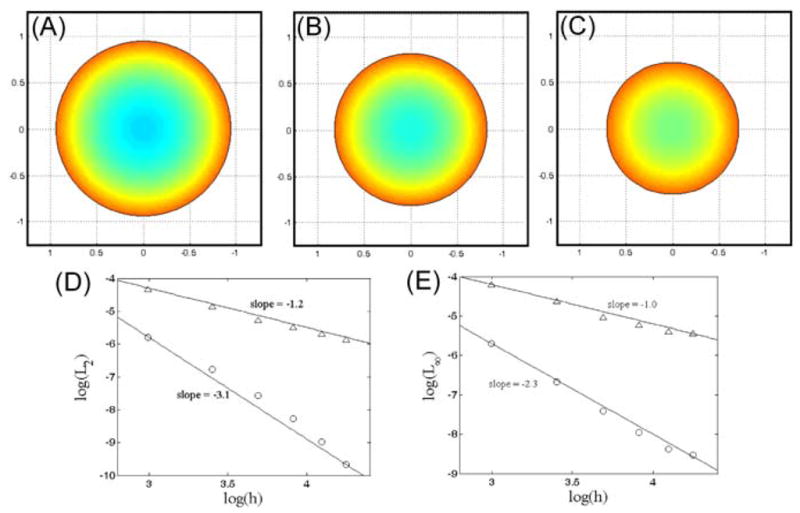
Reaction-diffusion of a chemical species with a physics-driven boundary. Decay of a chemical species causes the domain to shrink. The boundary velocity is proportional to the normal component of the gradient of the chemical species at the boundary. Solution at time t = 0.1 (A), t = 0.3 (B), and t = 0.5 (C). Colorscale varies between 0.8 (blue) and 1.4 (red). The L2 (D) and L∞ (E) errors as a function of grid spacing. Using the discretization of the derivative given in Sec. 2.2.3 leads to first order convergence (triangles), whereas a second order finite difference approximation of the normal component of the gradient gives second order convergence (circles).
| (67) |
Using this method to calculate the normal component of ∇C, we find better accuracy and roughly 3rd order convergence to the highly resolved solution (Fig. 6d).
3.5 Cell crawling powered by depolymerization
As mentioned in the Introduction, eukaryotic cell crawling is a complex process where biochemical reactions inside the cell are coupled to the biophysical mechanisms that move and deform the cell. Therefore, to construct realistic models for cell motility requires simulating reaction-diffusion equations inside a moving boundary. In this section, we develop a simple model for cell motility and show that our moving boundary algorithm provides a useful numerical scheme for addressing these kinds of problems.
Some of the simplest crawling cells are the spermatozoa from nematodes [46]. The sole function of these cells is the transport of genetic material. Indeed, the crawling sperm cell ejects many cellular components prior to activating. Therefore, these cells may represent a fundamental, stripped-down crawling motility apparatus. As in other crawling cells, motility is driven by a meshwork of polymer filaments. In place of actin filament, however, nematode sperm use a cytoskeleton composed of Major Sperm Protein (MSP). Polymerization of MSP at the leading edge of the cell pushes the front edge of the cell forward. The mechanism that the cell uses to adhere to the substrate is unknown, but recent experiments show that the adhesion at the front of the cell is stronger than at the rear [15]. In vitro experiments using cell-free extracts have suggested that depolymerization of the MSP network is responsible for producing the force that hauls the rear of the cell forward [14], and biophysical models for depolymerization-driven contraction of the MSP cytoskeleton agree well with experimental data [15,47]. In addition, recent experiments using Scanning Force Microscopy to measure forces produced by the actin cytoskeleton during the crawling of fish keratocytes also suggest that depolymerization may play a role in generating cytoskeletal flows in these cells [48]. Therefore, it is interesting to explore what shapes are produced by a depolymerization-driven model of cell motility.
In [15], a model for depolymerization of MSP was used to analyze experiments that related the size and shape of crawling cells to the translational velocity. Results suggested that the MSP filaments behave like a depolymerizing, anisotropic, linearly elastic solid. In that model, effects of the cytoskeleton and the cytosolic fluid were taken into account. To test our algorithm with the simplest cell crawling mechanism, we ignore the cytosolic effects. We work in terms of the MSP volume fraction, φ. If adhesion between the substrate and the cytoskeleton acts as a resistive drag, then the polymer velocity is proportional to the divergence of a stress, ζ vp = ∇ · σ, where ζ (x) is a drag coefficient that can depend on the spatial coordinates. The stress is assumed to be linear in φ, diagonal, and anisotropic [15],
| (68) |
where σ0 is the hydrostatic compressibility, φ0 is the equilibrium volume fraction, and α is the anisotropy. The dynamics for φ are given by the continuity equation augmented by depolymerization at rate γ. Linearization of this equation about φ ≈ φ0 leads to
| (69) |
Experimental evidence suggests that there is a sharp transition between high and low drag between the cytoskeleton and the substrate. To model this we use a drag coefficient given by
| (70) |
where C1 and C2 are constants. For our simulations, we use C1 = 5 and C2 = 25. Here, R is the distance from the center of an ellipse,
| (71) |
with (x0, y0) the position of the rear of the cell, and β defines the eccentricity of the ellipse. Δ1 defines the distance from the rear of the cell to the roll over from high to low drag, and λ1 is the width of this rollover region. For all of our simulations, λ1 = 0.2.
The surface tensions in the membrane of crawling cells has been estimated previously [15,21]. The values obtained suggest that the surface tension is small compared to the stresses generated in the cytoskeleton. We assume, though, that the cell has a preferred area (or volume in 3D), A0. Deviations from this area induce stress in the polymer. Therefore, Laplace’s law at the boundary is
| (72) |
where Γ is a constant. This boundary condition defines φ at the boundary.
The motion of the boundary is driven by two effects, polymerization of the MSP and motion of the existing polymer. We assume that the polymerization of the MSP at the boundary pushes out in the direction normal to the boundary and has a spatially-dependent magnitude, Va. Therefore, the normal component of the velocity at the boundary of the cell is
| (73) |
We assume that Va is positive at the front of the cell and zero near the rear,
| (74) |
For our simulations, we used that C3 = 0.1, Δ2 = 1.6, and λ2 = 0.5.
We solved Eq. 69 on a periodic, 50 × 50 grid of size 2 × 2 with a time step Δt = 0.05. We used an initial condition of a unit circle with φ = φ0 everywhere. The location of the center of the ellipse given by R is tracked by moving the point (x0, y0) with the average velocity of the cell. To see how the placement of the rollover in the substrate adhesion affects the cell shape during crawling, we ran simulations with Δ1 = 1.2 and 0.7. The former case places the rollover in drag past the center of the circle. We find that with these conditions the dynamics quickly produce a shape that is slightly pointed near the rear and is convex everywhere along the boundary (Fig. 7). The shape steadily translates and its globally convex boundary make it crudely similar to the shape of a crawling nematode sperm cell.
Fig. 7.

Simulation of a crawling cell driven by depolymerization. Panels (a)–(l) are evenly spaced time intervals of a simulated crawling cell. The colormap shows the volume fraction. Contours of the distance map and the boundary velocity (arrows) are also shown. The star shows the position of the rear of the cell. This simulation uses Δ1 = 1.2. Note that the rear of the cell is convex.
For the case when the drag rollover is closer to the rear of the cell, Δ 1 = 0.7, we also find that the cell quickly reaches a steadily-translating shape. In this simulation, because we track the position of the rear of the cell (x0, y0), using the average velocity, the point (x0, y0) detaches from the true back of the cell. This acts to make the rollover in the drag even closer to the back of the cell. Interestingly, the rear of the cell becomes concave, and the overall morphology resembles a half-moon. This shape is characteristic of crawling keratocytes [22,49,50]. Even though actin depolymerization has not been suggested as a force-producing mechanism in these cells, any bulk contraction may behave in a similar fashion [51]. In keratocytes, myosin II contraction at the rear of the cell may act to reduce the effective drag close to the rear of the cell [52]; therefore, this localization of lower drag may be responsible for the concavity of the back of the cell.
3.6 Cellular chemotaxis oriented by balanced inactivation
Many crawling cells are chemotactic. Cells sense their environment and move toward or away from chemical signals. As mentioned in the Introduction, receptors in the cell membrane activate membrane bound proteins, which begin a signalling cascade that locally triggers or enhances actin polymerization. The activation of membrane bound proteins has been shown to amplify the external signals, which allows cells to measure very small chemical gradients. For example, neutrophils and Dictyostelium discoideum cells can measure a concentration difference of roughly 1% across the length of the cell [53,54]. One strength of our algorithm is that at the boundary nodes lie explicitly on the boundary. Therefore, it is easy to couple chemical reactions between membrane bound speices with cytosolic factors, which is not true for algorithms that use cut cells and ghost points to represent the sharp interface [19].
To illustrate the applicability of our algorithm to these types of problems, we consider a simple chemical system that has been proposed as a mechanism for directional sensing during eukaryotic chemotaxis, which is known as a balanced inactivation model [55]. A strength of this model is that it captures a number of features of directional sensing, such as adaptation and the response of a cell in a high background of signal, which are not captured in other chemotaxis signalling models.
The balanced inactivation model proposes that chemical signal outside of the cell, denoted by S, triggers the cleavage of a membrane bound protein into a component that remains on the membrane, A, and a component that is released into the cytoplasm, B. The cytosolic component can diffuse with diffusion constant D and rebind to the membrane with rate kb, thereby becoming the membrane bound species Bm. Diffusion of the membrane bound species is assumed to be negligible. On the membrane, species A and Bm spontaneously degrade with rates k−a and k−b, respectively. In addition, species Bm can bind to A with a rate constant ki. This reaction inactivates species A. Therefore, the time evolution of the chemical species are given by
| (75) |
where ka is the rate constant for cleaving the membrane bound component. To account for production and binding of B to the membrane, the boundary condition for the final equation is
| (76) |
This model was solved previously on a stationary circular boundary [55]. If the background signal concentration is uniform, S = S0, then it can be shown analytically that the steady state values of the chemical species are
| (77) |
Here, we set out to determine the equilibrium shape that is generated by this model and the dynamic response of the cell morphology upon a rapid change in the external signal gradient. We assume that the concentration of A determines the polymerization rate of actin at the membrane. If actin polymerization is predominantly normal to the boundary, then the polymerization of actin will push the boundary in the normal direction. In addition, we define a preferred contact area between the cell and the substrate, a0, since cells are observed to maintain a fairly constant area (i.e., a0 is the 2D area of the cell). Therefore, we set the boundary velocity of the cell to be
| (78) |
where V0 and β are constants and a is the total contact area of the cell and the substrate. Motion of the cell membrane generates a flow of the cytosolic fluid, vf, which transports any cytosolic proteins. We model this flow using the methods described in Sec. 2.5. With the addition of this cytosolic velocity, the time evolution equation for B becomes
| (79) |
with boundary condition
| (80) |
We solved the Balanced Inactivation equations on an initially circular domain of diameter 5 μm in a linear signal gradient given by
| (81) |
with S0 = 10 and R being the radius of the cell. We used V0 = 0.0625 μm/s and α = 25 μm/s. The other parameters of the model are taken directly from the original paper [55]; i.e., ka = 1 s−1, ki = 1000 μm (s molecule)−1, kb = 3 μm/s, k−a = 0.2 s−1, k−b = 0.2 s−1, and D = 10 μm2/s.
Our first scenario simulates a cell in a fixed, constant signal gradient. We solve the equations on a 10 μm × 10 μm (101 × 101 nodes) grid, using a fixed time step of 0.005 sec. The only nonlinearities in this system come in the reaction rates of the membrane bound components. Therefore, we used a 2nd order Runge-Kutta algorithm to integrate the membrane bound components (first two equation in (75)) and used the fully implicit version of our algorithm, described in Sec. 2, to evolve the cytosolic concentration B. As our simulations are done on a periodic domain, we adjust the gradient as the cell crawls in order to maintain the correct signal concentration on the periodic domain. We find that the initially circular shape stretches out as the cell begins to crawl up the gradient (Fig. 9a–d). The cell takes on a tear drop shape, and the rear pulls forward slightly before the cell reaches a steady translating shape (Fig. 9e–h). The black arrows in Fig. 9 show the boundary velocity, which is linearly related to concentration of species A. The cell quickly polarizes with a high concentration of A developing from the slightly higher concentration of signal at the top portion of the cell. It is interesting to note that the polarization and magnitude of the concentration of A reaches a steady state, even though the absolute concentration of the external signal increases as the cell crawls. This is a realistic feature of the Balanced Inactivation model that is not captured by lateral excitiation/global inhibition models. The model produces shapes that are extended in the direction of motion; however, they are not overly reminiscent of the actual crawling of D. discoideum cells, which have a more uniform width. Clearly, a more accurate model for the internal dynamics of the cytoskeleton is needed to capture the actual morphology of Dictyostelium.
Fig. 9.

Simulation of a crawling cell driven by the Balanced Inactivation model in a linear external chemical gradient. Panels correspond to evenly spaced intervals of time with 9 sec between frames. (a)–(l) The cell begins with a circular shape in a gradient that increases toward the top of the page. The cell stretches and eventually becomes tear drop-shaped. The rear of the cell pulls up slightly as the cell reaches a steady crawling shape. The internal colormap shows the concentration of the diffusing cytosolic protein B. The black arrows show the boundary velocity (proportional to the concentration of species A as in Eq. 75), and the green arrows show the internal cytosolic velocity.
To explore how the shape of a cell driven by the Balanced Inactivation model responds to a time-dependent gradient, we model an initially circular cell that is in an initially constant gradient of external signal. Between times 15–19 seconds, the gradient is switched to point in the opposite direction (Fig. 10). Within less than 10 seconds of reversing the gradient, the cell begins to crawl in the new direction. Interestingly, the final morphology is half-moon shaped and reminiscent of a keratocyte, as opposed to the tear-drop shaped morphology that is observed during the crawling stages in a constant gradient (compare Fig. 9 and Fig. 10).
Fig. 10.

Simulation of a crawling cell driven by the Balanced Inactivation model in a linear external chemical gradient that switches direction. Panels correspond to evenly spaced intervals of time with 3.75 sec between frames. (a)–(d) The cell begins with a circular shape in a gradient that increases toward the top of the page. (e) Between 15–19 seconds, the direction of the gradient is switched to point in the opposite direction. Panels (f–l) show the response of the cell to the change in the external gradient. The background coloring shows the external chemical gradient. The internal colormap shows the concentration of the diffusing cytosolic protein B. The black arrows show the boundary velocity, and the green arrows show the internal cytosolic velocity.
These simulations show that the Moving Boundary Node Method can handle simulations where reactions between membrane bound and cytosolic proteins drive cell motility. Therefore, this method is well-suited for handling many problems that will arise during eukaryotic cell migration.
4 Comparison to other methods
Our algorithm is not the only numerical method for solving PDEs inside moving boundaries. In this section, we compare our method to some of the existing methods that can also be used to solve these types of problems.
For any moving boundary problem, a method must be chosen for defining the location of the boundary as a function of time. The two main methods for defining the position of the boundary are material point methods, such as the immersed boundary method [24], and level set methods [27,28]. A material point method defines the position of fixed points on a boundary and then evolves the positions of these points using the local velocity of the boundary. A major advantage of this method is that the new positions of the material points are easily calculated from the given velocity. However, care must be taken to prevent a chain of material points from crossing itself, to form loops. Typically, spring-like interactions are used to maintain a fixed connectivity between the material points. Two further drawbacks material point methods are that they do not handle merging or splitting of boundaries (such as might occur during cell fusion or division) and geometric properties of the boundary that are computed numerically, such as the normal direction and curvature, are prone to numerical errors that can lead to instabilities.
The level set method is an attractive alternative method that is widely used. The distance map representation of the boundary allows accurate calculation of geometric properties of the boundary and the implicit description of the boundary easily handles merging or splitting of boundaries. The primary drawback to the level set method is that reinitialization and high order methods (such as WENO) need to be employed to preserve the quality of the distance map [28], and time stepping is more computationally intensive than material point methods, since the boundary is represented by a function that lives in a higher-dimensional space. For problems in cell motility, the geometric properties of the boundary are important, and there are often cases where maintaining the connectivity of material points might be difficult, such as in the retraction of a long, thin fillipodium. Therefore, we opted to use the level set method to track the boundary of moving cells in our algorithm. Other groups have also begun to use the level set method to track the boundary of motile cells obtained from experimental images [37], to compute membrane diffusion [38], to model tumor growth [31], and to model chemotaxis in crawling cells [39]. Building on the strengths of the level set method, we then use the geometric information stored in the distance map to construct the finite volume representation of the computational domain; i.e., no additional calculation are required to determine the boundary nodes that are used in our method.
Level set methods have been used to solve bulk physical equations inside moving boundaries without displacing grid nodes. These methods typicaly rely on using ghost nodes that lie outside the boundary. For example, Fedkiw, et al. developed a ghost cell method for multimaterial flows [30] and similar methods have been applied to solve tumor growth models [40,31]. These methods do not provide nodes that lie on the boundary and mass conservation can be difficult to maintain. Because we use a finite volume discretization, mass conservation is natural. Unstructured grids [21] or body-fitted coordinates [41] could provide an equivalent finite volume representation but involve computationally intensive node redistribution after each boundary displacement. Instead, our method uses the distance map to reposition boundary nodes in a single step for each update leaving interior nodes on a fixed Cartesian grid.
A cut cell method [42] could also be used in place of our finite volume discretization. In these methods, the Cartesian grid is not modified; however, the contributions from grid cells that contain the boundary are approximated using the apertures that are computed from the boundary positions. The computational cost for computing these contributions is roughly comparable to the cost of computing the contributions from our distorted grids, and our method transparently avoids tiny control volume, which must be detected and eliminated in the cut cell method. In addition, cut cell methods do not provide nodes that lie on the boundary, which is also a drawback of adaptive mesh refinement [43]. During cell motility, membrane bound proteins often provide biochemical activation or inhibition of intracellular processes. Since the moving boundary node method provides explicit nodes on the boundary that are directly attached to interior nodes, it is straightforward to calculate membrane diffusion and biochemical reaction kinetics for chemical species on the membrane interacting with cytosolic proteins, which is not the case for cut cell methods. Indeed, our method also provides a method for solving for membrane diffusion that does not require spreading the membrane onto a higher-dimensional grid, as has been used recently [38,44].
A number of published alternatives combine finite volume and implicit surface methods, without moving nodes onto the boundary. Conveniences of these include the following: the potential for systematic extension to accuracy beyond second order [58]; accurate discretization of normal derivative jump boundary conditions [59]; direct application to medical imaging without complicated difference approximations for metric terms in surface derivatives [38]; and variable time steps for internal and surface nonlinear reaction terms [61]. However, the current implementations of these methods also come with a number of drawbacks, such as restriction to immobile surfaces [58,38,61] or, with loss of conservation form, rigidly translating surfaces [60]; diffusion restricted to either the surface [38] or the interior [58–61]; presumption of a quasi-steady state for interior reactions and diffusion [59]. Specialization makes alternatives to the Moving Boundary Node Method more advantageous for some problems but less advantageous for others. Straightforward hybridization has been proposed, almost universally, by the authors of each method, yet, at present, no single alternative can handle all the biologically relevant scenarios covered by the Moving Boundary Node Method (Section 3).
5 Conclusions
Here we have presented a finite volume-based algorithm for handling the dynamics of reaction-diffusion-advection equations inside a moving boundary. The boundary motion is tracked using standard level set method techniques, which provide a robust and accurate method for following physics-driven boundary displacements. In addition, the distance map provides the proper information to construct a discretization of irregular geometries using the nodes of a Cartesian grid; however, the procedure can lead to highly distorted quadrilateral areas near the boundary of the geometry. Therefore, to maintain second order accuracy in our spatial discretization, we consider the Taylor series expansion about the centers of the surface areas that enclose the finite volumes in our discretization. The Taylor series expansion couples neighboring points as well as nearest neighbors.
For the problems that we considered here, the most time consuming aspect of our algorithm was the reinitialization of the distance map. However, we did find that for large grids, the computational cost of constructing the matrices for the spatial discretization of the derivatives became the time limiting step. As we have not worked to optimize our algorithms, we have not systematically studied the optimal computational efficiency of the Moving Boundary Node Method.
One goal of this work was to construct a moving boundary algorithm that would maintain the total mass in a conservative system. Two aspects of our method are required to achieve this. First, because edge nodes are not located at the centers of their control volumes, time stepping can cause loss of mass at the geometry boundary. Therefore, the integral over a control volume that is associated with a node needs to be computed using subcontrol volume averages that are computed at the centers of the subcontrol volumes. Second, as our method gains and loses nodes as the boundary moves, an interpolation scheme is needed that preserves the total mass. We use a Laplacian integration scheme that is modified by a Lagrange multiplier to conserve the total amount of material inside the cell. The combination of these two procedures, conserves the total chemical mass inside the simulated geometry to roughly machine accuracy.
One field where we expect this method to be especially useful is in modeling eukaryotic cell motility. In these cells, complex biochemical reactions are coupled to the biophysical mechanisms that drive cell motility. Changes to the cellular biochemistry have been shown to lead to morphological changes in the crawling cell [56]. Feedback between the cell shape and the biochemistry are expected to be complex and will require good numerical methods for handling the moving boundary problem. In addition, conservation of the internal chemical components over the course of a simulation is imperative. Here we have shown that this algorithm can simulate the physics-driven motions of a simple model for cell motility. We show that the profile for the adhesion between the cell and the substrate may play a major role in determining the shape of a crawling cell. In addition, we have shown that the Balanced Inactivation model proposed in Levine, et al. can produce steady cell crawling in a fixed external chemical gradient.
The example simulations that we have done consider cellular motion driven by the presence of chemical species inside the cell. For simplicity, we have assumed that the concentration of the protein species at the boundary defines the normal component of the velocity. This assumption is not a requirement of our algorithm. Our algorithm can also handle cases where the protein species sets the tangential component of the velocity. For these cases, the tangential component of the velocity will not affect the displacement of the boundary nor the displacement of the boundary nodes. However, the protein species that are defined at or on the boundary will be advected by any tangential flows. These tangential velocities need only to be included in the advection matrices.
Fig. 8.

Simulation of a depolymerization-driven crawling cell with drag rollover closer to the rear of the cell. Panels (a)–(l) are evenly spaced time intervals. The colormap shows the volume fraction. Contours of the distance map and the boundary velocity (arrows) are also shown. The star shows the position of the rear of the cell. This simulation uses Δ1 = 0.7. The cell becomes “half-moon-shaped” and crawls at a steady rate.
Footnotes
Publisher's Disclaimer: This is a PDF file of an unedited manuscript that has been accepted for publication. As a service to our customers we are providing this early version of the manuscript. The manuscript will undergo copyediting, typesetting, and review of the resulting proof before it is published in its final citable form. Please note that during the production process errors may be discovered which could affect the content, and all legal disclaimers that apply to the journal pertain.
Contributor Information
Charles W. Wolgemuth, Email: cwolgemuth@uchc.edu, Department of Cell Biology and Center for Cell Analysis and Modeling, University of Connecticut Health Center, Farmington, CT 06030-3505.
Mark Zajac, Email: mzajac@alumni.nd.edu, Department of Mathematics, University of Utah, Salt Lake City, UT 84112.
References
- 1.Gupta SC. The Classical Stefan Problem: basic concepts, modeling and analysis. Elsevier Science; Amsterdam: 2003. [Google Scholar]
- 2.Chen S, Merriman B, Osher S, Smereka P. A simple level set method for solving Stefan problems. J Comput Phys. 1997;135:8–29. [Google Scholar]
- 3.Sethian JA, Strain JD. Crystal growth and dendritic solidification. J Comput Phys. 1992;98:231–253. [Google Scholar]
- 4.Gibou F, Fedkiw R. A fourth order accurate discretization for the Laplace and heat equations on arbitrary domains, with applications to the Stefan problem. J Comput Phys. 2005;202:577–601. [Google Scholar]
- 5.Karma A, Rappel WJ. Quantitative phase-field modeling of dendritic growth in two and three dimensions. Phys Rev E. 1997;57:4323–4349. [Google Scholar]
- 6.Lauffenburger DA, Horwitz AF. Cell migration: a physically integrated molecular process. Cell. 1996;84:359–369. doi: 10.1016/s0092-8674(00)81280-5. [DOI] [PubMed] [Google Scholar]
- 7.Mitchison TJ, Cramer LP. Actin-based cell motility and cell locomotion. Cell. 1996;84:371–379. doi: 10.1016/s0092-8674(00)81281-7. [DOI] [PubMed] [Google Scholar]
- 8.Rohatgi R, Nollau P, Ho H-YH, Kirschner MW, Mayer BJ. Nck and Phosphatidylinositol 4,5-Biphosphate synergistically activate actin polymerization through the N-WASP-Arp2/3 pathway. J Biol Chem. 2001;276:26448–26452. doi: 10.1074/jbc.M103856200. [DOI] [PubMed] [Google Scholar]
- 9.Le Clainche C, Pantaloni D, Carlier MF. ATP hydrolysis on actin-related protein 2/3 complex causes debranching of dendritic actin arrays. Proc Natl Acad Sci USA. 2003;100:6337–6342. doi: 10.1073/pnas.1130513100. [DOI] [PMC free article] [PubMed] [Google Scholar]
- 10.Mogilner A, Oster G. Force generation by actin polymerization II: the elastic ratchet and tethered filaments. Biophys J. 2003;84:1591–1605. doi: 10.1016/S0006-3495(03)74969-8. [DOI] [PMC free article] [PubMed] [Google Scholar]
- 11.Pollard TD, Blanchoin L, Mullins RD. Molecular mechanisms controlling actin filament dynamics in nonmuscle cells. Annu Rev Biophys Biomol Struct. 2000;29:545–576. doi: 10.1146/annurev.biophys.29.1.545. [DOI] [PubMed] [Google Scholar]
- 12.Vicente-Manzanares M, Zareno J, Whitmore L, Choi CK, Horwitz AF. Regulation of protrusion, adhesion dynamics, and polarity by myosins IIA and IIB in migrating cells. J Cell Biol. 2007;176:573–580. doi: 10.1083/jcb.200612043. [DOI] [PMC free article] [PubMed] [Google Scholar]
- 13.Huxley HE. Muscular contraction and cell motility. Nature. 1973;243:445–449. doi: 10.1038/243445a0. [DOI] [PubMed] [Google Scholar]
- 14.Miao L, Vanderlinde O, Stewert M, Roberts TM. Retraction in amoeboid cell motility powered by cytoskeletal dynamics. Science. 2003;302:1405–1407. doi: 10.1126/science.1089129. [DOI] [PubMed] [Google Scholar]
- 15.Zajac M, Dacanay B, Mohler WA, Wolgemuth CW. Depolymerization-driven flow in nematode spermatozoa relates crawling speed to size and shape. Biophys J. 2008;94:3810–3823. doi: 10.1529/biophysj.107.120980. [DOI] [PMC free article] [PubMed] [Google Scholar]
- 16.Mogilner A, Edelstein-Keshet L. Regulation of actin dynamics in rapidly moving cells: a quantitative analysis. Biophys J. 2002;83:1237–1258. doi: 10.1016/S0006-3495(02)73897-6. [DOI] [PMC free article] [PubMed] [Google Scholar]
- 17.Dawes AT, Edelstein-Keshet L. Phosphoinositides and Rho proteins spatially regulate actin polymerization to initiate and maintain directed movement in a one-dimensional model of a motile cell. Biophys J. 2007;92:744–768. doi: 10.1529/biophysj.106.090514. [DOI] [PMC free article] [PubMed] [Google Scholar]
- 18.Joanny JF, Julicher F, Prost J. Motion of an adhesive gel in a swelling gradient: a mechanism for cell locomotion. Phys Rev Lett. 2003;90:168102. doi: 10.1103/PhysRevLett.90.168102. [DOI] [PubMed] [Google Scholar]
- 19.Strychalski W. PhD Thesis. University of North Carolina; Chapel Hill: 2009. Simulation methods for spatiotemporal models of biochemical signaling networks. [Google Scholar]
- 20.Bottino D, Mogilner A, Roberts T, Stewert M, Oster G. How nematode sperm crawl. J Cell Sci. 2002;115:367–384. doi: 10.1242/jcs.115.2.367. [DOI] [PubMed] [Google Scholar]
- 21.Herant M, Marganski WA, Dembo M. The mechanics of neutrophils: synthetic modeling of three experiments. Biophys J. 2003;84:3389–3413. doi: 10.1016/S0006-3495(03)70062-9. [DOI] [PMC free article] [PubMed] [Google Scholar]
- 22.Rubinstein B, Jacobson K, Mogilner A. Multiscale two-dimensional modeling of a motile simple-shaped cell. Multiscale Model Simul. 2005;3:413–439. doi: 10.1137/04060370X. [DOI] [PMC free article] [PubMed] [Google Scholar]
- 23.Maree AFM, Jilkine A, Dawes A, Grieneisen VA, Edelstein-Keshet L. Polarization and movement of keratocytes: a multiscale modeling approach. Bull Math Biol. 2006;68:1169–1211. doi: 10.1007/s11538-006-9131-7. [DOI] [PubMed] [Google Scholar]
- 24.Peskin CS. The immersed boundary method. Acta Numerica. 2002;11:479–517. [Google Scholar]
- 25.Osher S, Sethian J. Fronts propagating with curvature dependent speed: Algorithms based on Hamilton-Jacobi formulations. J Comput Phys. 1988;79:12–49. [Google Scholar]
- 26.Sethian JA. Tracking interfaces with level sets. Am Sci. 1997;85 [Google Scholar]
- 27.Sethian JA. Level set methods and fast marching methods: evolving interfaces in computational geometry, fluid mechanics, computer vision, and material science. New York, NY: Cambridge University Press; 1999. [Google Scholar]
- 28.Osher S, Fedikiw R. Level set methods and dynamic implicit surfaces. New York, NY: Springer-Verlag; 2000. [Google Scholar]
- 29.Adalsteinsson D, Sethian JA. The fast construction of extension velocities in level set methods. J Comput Phys. 1999;148:2–22. [Google Scholar]
- 30.Fedkiw RP, Aslam T, Merriman B, Osher S. A non-oscillatory Eulerian approach to interfaces in multimaterial flows (the ghost fluid method) J Comput Phys. 1999;152:457–492. [Google Scholar]
- 31.Macklin P, Lowengrub J. Evolving interfaces via gradients of geometry-dependent interior Poisson problems: application to tumor growth. J Comput Phys. 2005;203:191–220. [Google Scholar]
- 32.Chung TJ. Computational Fluid Dynamics. Cambridge University Press; Cambridge, UK: 2002. [Google Scholar]
- 33.Zwart PJ, Raithby GD, Raw MJ. The integrated space-time finite volume method and its application to moving boundary problems. J Comput Phys. 1999;154:497–519. [Google Scholar]
- 34.Oosterom T, Oosterom A, Huiskamp G. Interpolation on a triangulated 3D surface. J Comput Phys. 1989;80:331–343. [Google Scholar]
- 35.Keren K, Yam PT, Kinkhabwala A, Mogilner A, Theriot JA. Intracellular fluid flow in rapidly moving cells. Nat Cell Biol. 2009;11:1219–1224. doi: 10.1038/ncb1965. [DOI] [PMC free article] [PubMed] [Google Scholar]
- 36.Novak IL, Gao F, Choi Y, Resasco D, Schaff JC, Slepchenko BM. Diffusion on a curved surface coupled to diffusion in the volume: Application to cell biology. J Computat Phys. 2007;226:1271–1290. doi: 10.1016/j.jcp.2007.05.025. [DOI] [PMC free article] [PubMed] [Google Scholar]
- 37.Machacek M, Danuser G. Morphodynamic profiling of protrusion phenotypes. Biophys J. 2006;90:1439–1452. doi: 10.1529/biophysj.105.070383. [DOI] [PMC free article] [PubMed] [Google Scholar]
- 38.Schwartz P, Adalsteinsson D, Colella P, Arkin AP, Onsum M. Numerical computation of diffusion on a surface. Proc Natl Acad Sci USA. 2005;102:11151–11156. doi: 10.1073/pnas.0504953102. [DOI] [PMC free article] [PubMed] [Google Scholar]
- 39.Yang L, Effler JC, Kutscher BL, Sullivan SE, Robinson DN, Iglesias PA. Modeling cellular deformations using the level set formalism. BMC Sys Biol. 2008;2:95. doi: 10.1186/1752-0509-2-68. [DOI] [PMC free article] [PubMed] [Google Scholar]
- 40.Astanin S, Preziosi L. Mathematical modeling of the Warburg effect in tumour cords. J Theor Biol. 2009;258:578–590. doi: 10.1016/j.jtbi.2009.01.034. [DOI] [PubMed] [Google Scholar]
- 41.Thompson J. Numerical grid generation: Foundations and applications. Elsevier; New York, NY: 1985. [Google Scholar]
- 42.Ji H, Lien FS, Yee E. An efficient second-order accurate cut-cell method for solving the variable coefficient Poisson equation with jump conditions on irregular domains. Int J Numer Meth Fluids. 2006;52:723–748. [Google Scholar]
- 43.Tang HZ, Tang T. Adaptive mesh methods for one- and two-dimensional hyperbolic conservation laws. SIAM J Numer Anal. 2003;41:487–515. [Google Scholar]
- 44.Adalsteinsson D, Sethian JA. Transport and diffusion of material quantities on propagating interfaces via level set methods. J Comput Phys. 2003;185:271–288. [Google Scholar]
- 45.Johansen H, Colella P. A cartesian grid embedded boundary method for Poisson’s equation on irregular domains. J Comput Phys. 1998;147:60–85. [Google Scholar]
- 46.Roberts TM, Stewert M. Nematode sperm amoeboid movement without actin. Trends Cell Biol. 1997;7:368–373. doi: 10.1016/S0962-8924(97)01113-6. [DOI] [PubMed] [Google Scholar]
- 47.Wolgemuth CW, Miao L, Vanderlinde O, Roberts T, Oster G. MSP dynamics drives nematode sperm locomotion. Biophys J. 2005;88:2462–2471. doi: 10.1529/biophysj.104.054270. [DOI] [PMC free article] [PubMed] [Google Scholar]
- 48.Goegler M, Käs JA, Ehrlicher A, Kock D, Wolgemuth CW, Brunner C. The origin and spatial distribution of forces in motile cells. Cell. submitted. [Google Scholar]
- 49.Grimm HP, Verkhovsky A, Mogilner A, Meister JJ. Analysis of actin dynamics at the leading edge of crawling cells: Implications for the shape of keratocyte lamellipodia. Eur Biophys J. 2003;32:563–577. doi: 10.1007/s00249-003-0300-4. [DOI] [PubMed] [Google Scholar]
- 50.Keren K, Pincus Z, Allen GM, Barnhart EL, Marriott G, Mogilner A, Theriot JA. Mechanism of shape-determination in motile cells. Nature. 2008;453:475–480. doi: 10.1038/nature06952. [DOI] [PMC free article] [PubMed] [Google Scholar]
- 51.Wolgemuth CW. Lamellipodial contractions during crawling and spreading. Biophys J. 2005;89:1643–1649. doi: 10.1529/biophysj.105.066720. [DOI] [PMC free article] [PubMed] [Google Scholar]
- 52.Svitkina TM, Verkhovsky AB, McQuade KM, Borisy GG. Analysis of actin-myosin II system in fish epidermal keratocytes: Mechanism of cell body translocation. J Cell Biol. 1997;139:397–415. doi: 10.1083/jcb.139.2.397. [DOI] [PMC free article] [PubMed] [Google Scholar]
- 53.Zigmond SH. Ability of polymorphonuclear leukocytes to orient in gradients of chemotactic factors. J Cell Biol. 1977;75:606–616. doi: 10.1083/jcb.75.2.606. [DOI] [PMC free article] [PubMed] [Google Scholar]
- 54.Song L, Nadkarni SM, Bödeker HU, Beta C, Bae A, Franck C, Rappel WJ, Loomis WF, Bodenschatz E. Dictyostelium discoideum chemotaxis: threshold for directed motion. Eur J Cell Biol. 2006;85:981–989. doi: 10.1016/j.ejcb.2006.01.012. [DOI] [PubMed] [Google Scholar]
- 55.Levine H, Kessler DA, Rappel WJ. Directional sensing in eukaryotic chemotaxis: a balanced inactivation model. Proc Natl Acad Sci USA. 2006;103:9761–9766. doi: 10.1073/pnas.0601302103. [DOI] [PMC free article] [PubMed] [Google Scholar]
- 56.Lacayo CI, Pincus Z, VanDujin MM, Wilson CA, Fletcher DA, Gertler FB, Mogilner A, Theriot JA. Emergence of large-scale cell morphology and movement from local actin filament growth dynamics. PLos Biology. 2007;5:e233. doi: 10.1371/journal.pbio.0050233. [DOI] [PMC free article] [PubMed] [Google Scholar]
- 57.Elliott C, Stinner B. Analysis of a diffuse interface approach to an advection diffusion equation on a moving surface. Math Mod Meth Appl S. 2009;19:787–802. [Google Scholar]
- 58.Ligocki TJ, Schwartz PO, Percelay J, Colella P. Embedded boundary grid generation using the divergence theorem, implicit functions, and constructive solid geometry. J Phys Conf Ser. 2008;125:012080. [Google Scholar]
- 59.Macklin P, Lowengrub J. A New Ghost Cell Level Set Method for Moving Boundary Problems: Application to Tumor Growth. J Sci Comput. 2008;35:266–299. doi: 10.1007/s10915-008-9190-z. [DOI] [PMC free article] [PubMed] [Google Scholar]
- 60.McCorquodale P, Colella P, Johansen H. A Cartesian Grid Embedded Boundary Method for the Heat Equation on Irregular Domains. J Comput Phys. 2001;173:620–635. [Google Scholar]
- 61.Strychalski W, Adalsteinsson D, Elston TC. A cut cell method for simulating spatial models of biochemical reaction networks in arbitrary geometries. Comm App Math and Comp Sci. 2010;5:31–53. doi: 10.2140/camcos.2010.5.31. [DOI] [PMC free article] [PubMed] [Google Scholar]
- 62.Teigen KE, Li X, Lowengrub J, Wang F, Voigt A. A diffuse-interface approach for modeling transport, diffusion and adsorption/desorption of material quantities on a deformable interface. Commun Math Sci. 2009;7:1009–1037. doi: 10.4310/cms.2009.v7.n4.a10. [DOI] [PMC free article] [PubMed] [Google Scholar]