Characterization of Exposures to Airborne Nanoscale Particles During Friction Stir Welding of Aluminum

Abstract

Friction stir welding (FSW) is considered one of the most significant developments in joining technology over the last half century. Its industrial applications are growing steadily and so are the number of workers using this technology. To date, there are no reports on airborne exposures during FSW. The objective of this study was to investigate possible emissions of nanoscale (<100 nm) and fine (<1 μm) aerosols during FSW of two aluminum alloys in a laboratory setting and characterize their physicochemical composition. Several instruments measured size distributions (5 nm to 20 μm) with 1-s resolution, lung deposited surface areas, and PM_2.5 concentrations at the source and at the breathing zone (BZ). A wide range aerosol sampling system positioned at the BZ collected integrated samples in 12 stages (2 nm to 20 μm) that were analyzed for several metals using inductively coupled plasma mass spectrometry. Airborne aerosol was directly collected onto several transmission electron microscope grids and the morphology and chemical composition of collected particles were characterized extensively. FSW generates high concentrations of ultrafine and submicrometer particles. The size distribution was bimodal, with maxima at ∼30 and ∼550 nm. The mean total particle number concentration at the 30 nm peak was relatively stable at ∼4.0 × 10⁵ particles cm⁻³, whereas the arithmetic mean counts at the 550 nm peak varied between 1500 and 7200 particles cm⁻³, depending on the test conditions. The BZ concentrations were lower than the source concentrations by 10–100 times at their respective peak maxima and showed higher variability. The daylong average metal-specific concentrations were 2.0 (Zn), 1.4 (Al), and 0.24 (Fe) μg m⁻³; the estimated average peak concentrations were an order of magnitude higher. Potential for significant exposures to fine and ultrafine aerosols, particularly of Al, Fe, and Zn, during FSW may exist, especially in larger scale industrial operations.

INTRODUCTION

Motivation

The original motivation for this study was to determine an effective approach for characterizing exposures of students and researchers to engineered and incidental nanoparticles in university laboratory settings, consistent with the recommendation that the nanotechnology community develop a compendium of information on airborne release fractions, respirable fractions, and biologically relevant particle characteristics for representative research, development, and nanomanufacturing processes (Hoover et al., 2007). Friction stir welding (FSW) was selected as the process of interest for this study because of the paucity of exposure data on this new technology and the collateral objective of investigating potential environmental health and safety advantages of FSW over traditional fusion welding.

The main objective of this study was to investigate potential emission of nanoscale aerosols generated during FSW and to assess its key physicochemical properties. A longer term goal is to conduct a comparative assessment of several research grade (very expensive and bulky) and practitioner grade (inexpensive and portable) aerosol instruments under realistic workplace conditions in order to identify suites of essential instruments necessary for adequate characterization of fine and ultrafine aerosols, especially from the standpoint of a practicing occupational hygienist.

FSW

FSW, considered one of the most significant developments in joining technology over the last half century (Nishikawa and Fujimoto, 2004), falls into the category of solid-state welding because it creates a joint without melting the workpiece. A report by Miller et al. (2002) on seven industry sectors within the manufacturing, construction, and mining industries, which account for approximately one-third of the total U.S. Gross Domestic Product, found that these seven sectors alone spent $34.1 billion on welding in 2000. An ever increasing fraction of welding is done with the FSW process, invented at The Welding Institute in the United Kingdom in 1991 (Thomas et al., 1991). The ability of FSW to economically produce high-quality welds in all aluminum alloys, including welding of dissimilar materials, and its potential for welding high-melting-point metals has made it an attractive alternative to other joining processes. A growing number of workers potentially use FSW in a range of industry sectors, including aerospace (Christner et al., 2003a; Christner et al., 2003b; Schortt, 2003; Colegrove, 2007), automotive (Smith et al., 2001; Schortt, 2003; Smith et al., 2003), railway (Kalle et al., 2002), armored vehicle (Colligan et al., 2003), and shipbuilding (Przydatek, 1999; Smith, 2000; Konkol et al., 2003; Lienert et al., 2003; Posada et al., 2003; Lienert, 2004; Halverson et al., 2006).

The basic concept of FSW can be described as follows: a nonconsumable rotating FSW tool with a specially designed shoulder and pin is pressed against the base metal surface, while a vertical downward force is applied (Fig. 1). Due to friction between the rotating tool and the workpiece, the temperature in the weld zone increases. The generated heat is not sufficient to melt the material (the weld zone temperature usually reaches 80–95% of the material’s melting point). However, the workpiece is softened in the area around the pin and the deformation resistance (i.e. yield strength) of the base material decreases. The rotating tool transports plasticized material from the advancing side to the rear of the tool (like extrusion) and forges it on the backside, creating a joint. With the pin fully penetrated and the shoulder riding on the top surface of the workpiece, the tool is traversed along the seam. Mishra and Ma (2005) has written an excellent review paper on the process.

Fig. 1.

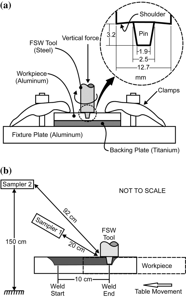
Schematic of FSW apparatus: (a) tool and workpiece geometry and (b) sampling geometry.

In contrast to conventional fusion welding methods, FSW occurs below the material’s melting temperature; it uses no shielding gases, requires little or no weld preparation, no filler materials, and uses much less energy. Its practitioners have assumed, because it is a solid-state welding process and no anecdotal evidence has surfaced to suggest otherwise, that there are no gaseous or aerosol emissions. Lack of published research on airborne aerosols produced by FSW was a major motivation for this study.

EXPERIMENTAL APPROACH

Because FSW results in significant rubbing of the outer surface of the tool against the workpiece, this may generate airborne aerosols. Aluminum alloys were chosen as workpieces because the majority of commercial FSW is done on these alloys (Smith, 2008). An initial site visit was conducted in August 2007 during which time preliminary data were collected on the nature and dynamics of the FSW process. From that preliminary investigation, it became apparent that fast responding instruments (∼1 s) and proper chemical characterization of emitted aerosols were critical requirements. The data for this study were collected during three subsequent days in August 2008.

FSW process

FSW was performed on a commercial three-axis computer numerically controlled mill (model TM-1 from HAAS Automation, Inc., Oxnard, CA). The experimental apparatus is shown in Fig. 1. A special welding fixture was mounted on the mill table to rigidly clamp the workpiece. A 76.2 × 152.4 mm titanium (Grade 5) backing plate was mounted under the workpiece to be welded. The FSW tool, made out of prehardened H13 tool steel, had a concave shoulder (12.7 mm diameter) and a threaded conical pin (3.2 mm long, tapering from 2.5 to 1.9 mm diameter).

The test matrix consisted of four cases involving workpieces of two different aluminum alloys (6061-T6 and 5083-H111), each welded at two different spindle speeds (summarized in Table 1). The same FSW tool and approximate weld depth were used in all tests. For all cases, simple bead-on-plate welds were generated along the same path (i.e. on top of each other) on a single workpiece. Preliminary measurements showed that subsequent weld passes in the same location of the workpiece did not change the quantity of emitted particles. In addition, unlike many other welding processes FSW does not significantly alter the chemistry or microstructure in the weld nugget. Each weld was 100 mm long and the tool was in contact with the workpiece for 40 s. The minimum time interval between welds was 4 min.

Table 1.

FSW process parameters^a

	Case 1A	Case 1B	Case 2A	Case 2B
Workpiece	6061-T6 aluminum		5083-H111 aluminum
Plunge depth (mm)	2.9		3.0
Spindle speed (r.p.m.)	1500	900	1500	900
Feed rate (mm min−1)	200
Weld power input (W)	1218 ± 77	1081 ± 82	1315 ± 150	1031 ± 153

^aThe workpiece thicknesses, 3.175 and 5.080 mm for the 6061-T6 and 5083-H111 alloy samples, respectively, was not considered a variable of influence for the study. The same FSW tool and approximate weld depth were used in all tests. The slightly different plunge depths should not be interpreted as another variable in the context of this study but instead as an integral part of the choice of workpiece material and is reflective of complex interactions of the workpiece with the milling machine.

Instrumentation for airborne particle measurement

Seven real-time instruments, divided into two suites (research or practitioner grade) based on the nature and quality of their data, were used to measure the airborne particles emitted during the FSW process. Table 2 lists the instruments, along with a brief description and the pertinent measurement specifications.

Table 2.

Summary of instrumentation used for characterization of airborne particles

Instrument		Specifications
Name (model)a	Measures	Response time (s)	Size range (μm)	Channels	Collection efficiency	Upper range
Suite 1: real-time samplers
EEPS (TSI 3090)	Size distribution and TNC, electrical mobility diameter	1	0.0056–0.56	32	Size dependent	>1.0 × 106 cm−3
APS (TSI 3321)	Size distribution and TNC, aerodynamic diameter	1	<0.5 to 20	52	Size dependent	1.0 × 104 cm−3
NSAM (TSI 3550)	TB and A lung deposited surface area concentration	1	0.01–1	—	Size dependent	2.5 × 103 (TB); 1.0 × 104 (A), μm2 cm−3
DustTrak, PM2.5 inlet (TSI 8520)	Mass concentration (particle diameter <2.5 μm)	1	0.10–2.5	No size resolution		100 mg m−3
Suite 2: real-time samplers
DustTrak, PM1.0 inlet (TSI 8520)	Mass concentration (particle diameter <1.0 μm)	1	0.10–1	No size resolution		100 mg m−3
CPC (TSI 3007)	TNC	1	0.010−1	No size resolution	Size dependent	∼1.0 × 105
P-Trak (TSI 8525)	TNC	1	0.020–1	No size resolution	Size dependent	∼5.0 × 105
Integrated samplers
TP (Fraunhofer Institute of Toxicology, Germany)	Collects particles on a TEM grid over a predefined time period using a thermal gradient	NA	Broad:0.001 to >100	No size resolution	Size dependent, highest for nanoparticles	—
ESP(courtesy of Dr A. Miller, NIOSH)	Collects particles on a TEM grid over a predefined time period using a point-to-plane electrostatic corona discharge	NA	Broad:0.001>100		>80 (at 20 nm) to 100% (at 400 nm)
WRASS (Naneum Ltd)	Collects and sizes the aerosol over a wide size range (0.002–20 μm) in 12 stages, 5 of which are in the 0.002–250 nm range. Subsequent chemical analysis on stages enables construction of size distributions of analyte of interest	NA	0.002–20	12 stages	<0.2% penetration	—
Personal respirable sampler (GK 2.69 cyclone; BGI Inc., Waltham, MA, USA)	Collects respirable dust (1–10 μm) when operated at 4.2 l min−1	NA	1–10	—	Size dependent; follows the respirable fraction convention	—
PM2.5 sampler (PEM Model 200; MSP Inc.)	Collects respirable dust (<2.5 μm) on a 37-mm PVC filter using a single-stage inertial impactor at 4 l min−1	NA	<2.5	—		—

PVC, polyvinyl chloride.

^aTP stationed at the BZ; ESP stationed near the source. WRASS, an area sampler, was positioned at BZ height next to the operator. PM_2.5 was operated as an area sampler. Suite 1 is made of research grade instruments (except for DustTrak), whereas Suite 2 is made of practitioner grade instruments.

Real-time aerosol characterization

Two research grade continuous monitoring instruments were used to capture the particle size distribution and number concentration of the generated aerosols: an Engine Exhaust Particle Sizer™ (EEPS model 3090) and an Aerodynamic Particle Sizer (APS model 3321) both from TSI Inc. (St Paul, MN, USA). These instruments collectively cover a broad size distribution range of 5.6 nm to 20 μm and have a fast response time of one full size distribution sec⁻¹, a critical requirement for acquiring size distributions of transient processes. The EEPS uses unipolar diffusion charging of particles and measures electrical mobility diameter in the 5.6–560 nm range in 32 channels, generating the size distribution and total number concentration (TNC), with an upper linear range of 1 million particles cm⁻³. The APS measures the size distribution and TNC in the range of 0.5–20 μm (aerodynamic diameter) in 52 channels based on the time-of-flight of particles in an accelerating flow field and provides usable data up to 10 000 particles cm⁻³. Additionally, we also used a nanoparticle surface area monitor (NSAM model 3550 by TSI, Inc.), which calculates the human lung-deposited surface area concentration of particles (in squared millimeters per cubic meter) corresponding to the tracheobronchial (TB) and alveolar (A) regions of the human lung. The NSAM relies on diffusion charging of particles, a property proportional to the surface area concentration, followed by their detection in an electrometer. The equivalent lung-deposited surface area concentration is then calculated using a standard lung deposition model over the 10–1000 nm range. This parameter represents an interesting dose metric for inhalation toxicology and exposure assessment purposes.

The practitioner grade real-time instruments [condensation particle counter (CPC) model 3007, P-Trak™ model 8525, and DustTrak™ model 8520 by TSI Inc.] are commonly used by practicing occupational hygienists. The CPC and P-Trak™ provide a single TNC (0.01–1 and 0.02–1 μm, respectively) with a 1-s response time but they lack size resolution. The DustTrak™ provides a mass concentration in the range of 0.1–10 μm and was operated with a PM_2.5 and PM_1.0 inlet.

The DustTrak™ measurements were calibrated to the average aerosol concentration from independent gravimetric measurements of a PM_2.5 sampler, which collected particles on 37-mm polyvinyl chloride (PVC) filters at 4 l/min, (PEM™ Model 200; MSP Inc., Minneapolis, MN, USA), using a calibration factor that was derived from ‘calibration factor = gravimetric concentration/time-integrated DustTrak™ concentration. Because no gravimetric sampling was conducted for PM_1.0, the calibration factor for PM_2.5 was also applied for PM_1.0 DustTrak™ measurements.

The samplers’ inlets, connected with 1-m long conductive tubing, were located at one of two positions behind the welding tool: (i) 20 cm from the weld zone (location of source emission) at a fixed vertical angle of ∼45 degrees and (ii) at the location of the FSW operator (with the operator present), 92 cm from the weld zone [breathing zone (BZ) of the operator]. The FSW tool (weld source) and sampling locations remained fixed in global coordinates; hence, their relative position with respect to each other was constant. Each suite of instruments (Table 2) measured the particle emissions at each sampling location five times for each case, by alternating their position after each test. A time stamp for each event was recorded to the laptop according to observer input using software developed for this purpose. For the purpose of data analysis, weld start was considered to be when the tool plunged into the workpiece, and weld end was the moment the tool retracted from the workpiece.

Integrated sampling

Particle morphology.

An electrostatic precipitator (ESP, courtesy of Dr A. Miller, National Institute for Occupational Safety and Health) and a thermophoretic precipitator (TP, Fraunhofer Institute of Toxicology, Germany) were employed to collect particles on transmission electron microscopy (TEM) grids for subsequent morphology and elemental analysis. These instruments use an electrical corona discharge and thermal gradient, respectively, as the collection mechanism. The sampling time for both instruments was set to approximate the duration of the process (2–3 min per test run) in order to minimize collection of background aerosol and 3–5 test cycles were sampled on the same grid. Four grids were collected from each instrument for a total of eight grids. The TP was operated at a probe temperature of 120°C and tip temperature of 38°C. The TEM grids (Electron Microscopy Sciences, Hatfield, PA, USA) were 200-mesh Cu with a silicon monoxide film. Electron microscopy imaging of particles on these grids is described in a subsequent section.

Chemical composition.

A wide range aerosol sampling system (WRASS, Naneum Ltd, Canterbury, UK) was used to collect size-selective fractions of the aerosol over the range of ∼2 nm to 20 μm in 12 stages. The principle of operation and performance of this new instrument are described in Gorbunov et al., (2009). The WRASS is a combination of a cascade impactor (seven stages, 0.25–20 μm) and a diffusion battery (five stages, 2–250 nm). Chemical analysis of each stage for select transition metals (Al, Zn, Fe, Cr, Mn, Mo, Co, Ni, and Zr) was performed with inductively coupled plasma mass spectrometry (ICP-MS) on an Agilent 7500cs ICP-MS system (Agilent Technologies, Yokogawa, Japan) based on the U.S. Environmental Protection Agency (EPA) method 3051A, which uses microwave-assisted acid digestion of samples.

BZ respirable dust (<10 μm) samples (one per day) were collected on the operator with a high-flow rate GK 2.69 respirable cyclone (BGI Inc., Waltham, MA, USA) operated at 4.2 l/min on a 37-mm PVC filter. Following gravimetric analysis of filters in a temperature- and humidity-controlled environmental chamber (Cahn C-30 microbalance; Cahn Instruments, Cerritos, CA, USA; 1-μg resolution), the PVC filters were analyzed by ICP-MS for the same set of metals listed above.

Electron microscopy analysis

Extensive electron microscopy analysis was performed to examine the morphology and chemistry of the particles generated during the welding process. The majority of the analyses were conducted in a high-resolution Hitachi S-5500 field emission scanning electron microscopy/scanning transmission electron microscope (STEM) (Hitachi High Technologies America, Inc., Pleasanton, CA, USA) at RJ Lee Group, Inc. The S-5500 has unique capabilities making it well suited to the study of the morphology and chemistry of nano-sized particles. At a maximum magnification of ×2 000 000 and a point resolution of 0.4 nm at 30 kV, particles 5–10 nm can be imaged. Most important for this study is the ability to simultaneously collect secondary electron images (SEIs), bright field or dark field STEM images, and energy dispersive x-ray spectroscopy (EDS) spectra without having to change the specimen position. The EDS spectra were collected with a 10 mm² XFlash® silicon drift detector at 35° takeoff angle and associated QUANTAX™ ED EDS software. The samples were coated with a thin (<10 nm) layer of carbon to prevent particles from popping off the grid as the beam built up charge on the particles during EDS acquisitions. As a result of the sample mount and film coating, C, O, Si, and Cu spectrum peaks are present as artifacts in each EDS spectrum and should be disregarded.

Statistical analysis

Raw data from the sampling instruments were first imported into spreadsheets. Process variables were created and the data were checked for accuracy using additional manual records from the field. The database was then exported into SPSS® (v17; SPSS Inc., Chicago, IL, USA) and SAS v9 (SAS Inc., Carry, NC, USA) for further data reduction and analysis.

The distributions of the TNCs from the real-time instruments were examined graphically via probability plots and histograms and were found to be lognormal. Hence, they were log-transformed and all analyses were conducted on the transformed data. Real-time data from all instruments were modeled using time series techniques as serial measurements of short duration (1–10 s) are expected to be highly autocorrelated. The autoregressive integrated moving-average (ARIMA) procedure in SAS was used to investigate the autocorrelation and to test autocorrelation coefficients at different time lags as well as to generate correlograms (plots of autocorrelation coefficients versus time lags) and partial autocorrelation plots. The plots showed a range of exposure patterns over time in the different processes, and significant autocorrelation coefficients were observed at different time lags, but all samples consistently demonstrated a significant autocorrelation coefficient at the first time lag (first order autoregressive process). Hence, summary statistics including the geometric mean (GM) and geometric standard deviation (GSD) were calculated for processes using the MIXED procedure in SAS and specifying the first order autoregressive correlation structure.

RESULTS

Process dynamics

Figure 2 shows a typical particles size distribution (dN/dLog Dp; particles cm⁻³) as a function of time (s) as measured by the EEPS and APS (Table 2) at the source of one weld (Case 1: 6061-T6 aluminum, 1500 r.p.m.). The FSW tool (Fig. 1) made first contact with the workpiece at 10 s and the shoulder engaged the surface at 20 s, after which the tool traversed across the workpiece and then retracted at 53 s. The highest concentrations of nanoparticles were measured during the traverse at 34 and 40 s for the APS and EEPS measurements, respectively. A broad peak in the >5 to 150 nm range with a single maxima at ∼30 nm was observed for the two EEPS-measured particle emission events during the FSW cycle (Fig. 2a). A detailed description of the size distribution over the whole monitored particle range is provided in the following section.

Fig. 2.

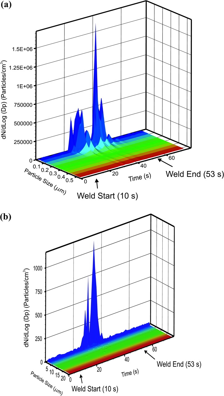
Typical size distribution (dN/dLog Dp, particle number per cubic millimeter) near the source for Case 1 as a function of time; (a) EEPS (Dp = electrical mobility diameter); (b) APS (Dp = aerodynamic diameter).

Particle size distribution

Figure 3 shows the averaged particle size distributions (dN/dLog Dp; particles cm⁻³) for the four cases, as measured by the EEPS and APS over a wide combined range of particle sizes (5.6 nm to 20 μm) at the BZ and near the source. EEPS measures the electrical mobility diameter, whereas the APS the aerodynamic diameter. These diameters may differ and the magnitude of this difference will depend on the type of aerosol (chemical composition, electrical properties, and shape factor). The sandwiching of the two distributions allows for easy visual comparisons of the particle number concentrations of different sizes. Each data point in Fig. 3 represents the channel-specific number concentration averaged over the duration of a weld and for all replicates of each case. The y-axis is in fact a relative number concentration. The error bars for the four curves on each graph are omitted for the purpose of clarity. The standard error of the mean for each process varied with the channel size and represented typically 5–30% of the channel mean number concentration value.

Fig. 3.

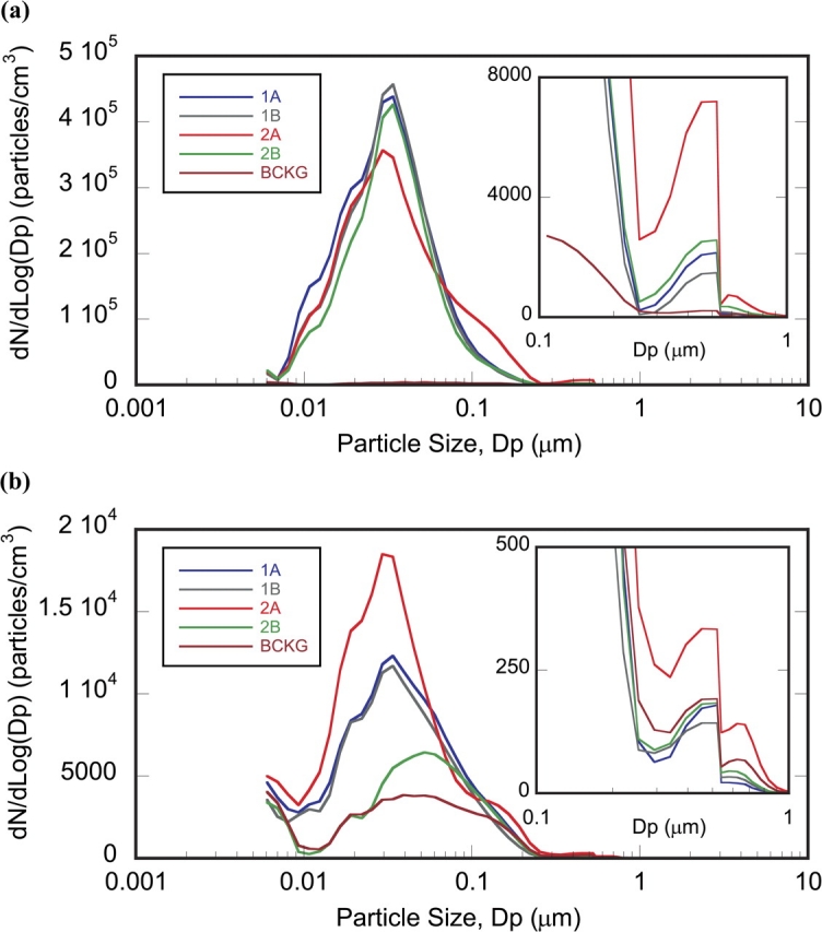
Average size distribution (dN/dLog Dp) at (a) source and (b) BZ. The y-axis represents the relative particle number concentration, whereas the x-axis the channel midpoint. Each data point is the arithmetic mean of that channel value over five replicate tests. Standard errors of the mean have been omitted for clarity purposes. The EEPS measures the electrical mobility diameter, whereas the APS the aerodynamic diameter. Little overlap between two size distribution ranges and the different principles for measuring Dp may explain the dip at ∼600 nm. Case 1A through 2B are defined in Table 1.

The source distribution was a single broad-base peak for all four cases with a maximum at ∼30 nm and mean counts at the maximum between 3.5 × 10⁵ (Case 1A) and 4.5 × 10⁵ particles cm⁻³ (Case 2A, Fig. 3a). A second broad peak was observed in the 0.1–1 μm range, with its maximum ∼550 nm (Fig. 3a, insert). The step decline in the size distribution of this second peak is partly an artifact of sandwiching of the data between the two instruments, with little overlapping between the two distributions at the maxima. An additional factor, further addressed in a subsequent section, may have to do with the fact that the two instruments use different principles to measure particle size, hence resulting in different concentrations. The mean particle number concentration at this second maximum varied between 1500 (Case 1B) and 7200 particles cm⁻³ (Case 2A). A larger variation was seen for the source size distribution and number concentration of the 550 nm maximum compared to the 30 nm maximum. The baseline size distribution (before each test) averaged over the 3 days of testing (better observed in Fig. 3b) reached a mean maximum of ∼3800 particles cm⁻³ at 125 nm. For the purpose of this study, baseline was defined as the time interval between two consecutive tests, whereas background is referred to as a time interval before any tests were conducted. In this regard, background concentration and distribution may not be affected by the process itself, whereas baseline distribution is affected by the process. The mean source number concentration for all four cases was at least 100 times greater than that of the background at the 30 nm maximum and ∼10–40 times greater at the 550 nm maximum. The broadening of the baseline peak to larger particle sizes (up to 500 nm) was likely a result of ongoing agglomeration of released nanoparticles as they transited to the BZ (also confirmed by electron microscopy). The background size distribution at the beginning of each day prior to any tests was narrower (i.e. very few particles >200 nm) than this daylong averaged baseline distribution.

The particle size distribution in the BZ was qualitatively similar to that in the source (one broad predominant peak with its maximum at ∼30 nm and a smaller peak with its maximum at ∼550 nm), but there was more variability in the data between cases. There was, however, a shift in the peak maximum toward larger particles for cases with lower concentrations, increasingly resembling baseline size distribution. Significantly more particles reached the BZ for Case 2A welds (5083-H111 at high r.p.m.) than for the other three cases. Case 2A had a mean peak concentration of 1.9 × 10⁴ particles cm⁻³ with a maximum at ∼30 nm (Fig. 3b). Cases 1A and 1B (6061-T6) had mean peak concentrations of 1.2 × 10⁴ particles cm⁻³ at the same particle diameter of 30 nm. Interestingly, while the high-r.p.m. test with 5083-H111 (Case 2A) had the highest mean particle concentrations at the BZ, the low-r.p.m. test for the same aluminum alloy (Case 2B) resulted in the lowest mean peak concentration (6450 particles cm⁻³) at a particle diameter of 52 nm (Fig. 3b). Case 2A was the only one that produced a higher concentration than background (mean peak of 330 versus 190 particles cm⁻³) at ∼550 nm (Fig. 3b).

Summary of totals from all instruments

Source.

Total instrument outputs (number and surface area concentration) from the several direct reading instruments are reported in Tables 3 and 4 for source and BZ locations, respectively. The TNCs during the various welding cases were significantly different from the background concentration, but not from each other, with the exception of APS data for Case 2A, which was significantly different from other cases. The GM TNC measured by EEPS varied between 2.1 and 3.5 × 10⁴ particles cm⁻³ (GSDs, 9–11), whereas the maximum TNC varied by case between 2.6 and 3.9 × 10⁶ particles cm⁻³. These GMs were about an order of magnitude higher than background. The cases were significantly higher than background but not from each other. The GM TNCs as measured by APS varied by case between 20 and 59 particles cm⁻³ (GSDs, 2.9–3.7), whereas the maxima varied from 739 to 3055 particles cm⁻³. As with the EEPS, all cases were different from background. Only case 2A was different from three other cases. The GM total lung deposited surface area concentration calculated by the NSAM varied from 138 to 291 μm² cm⁻³ (GSDs, 7.2–12.4) with maximum values ranging from 4737 to 19 000 μm² cm⁻³. Case 1A had the highest recorded maximum values for all instruments. The P-Trak data followed the EEPS data closely, except that it provided smaller estimates at high concentrations. This may be partially caused by the fact that the P-Trak has significant coincidence errors at higher concentrations (i.e. underreporting of actual particle concentration due to reporting of a single count when two or more particles are present in the measured volume). The P-Trak GM varied between 1.1 and 7.2 × 10⁴ (GSDs, 5.2–9.2) and the maximum values exceeded the upper linearity limit of the instrument for all cases. The GM DustTrak mass concentrations varied between 0.015 and 0.029 (GSDs, 3.6–5.9) mg m⁻³ or ∼2 to 4 times higher than the GM background level of 0.007 mg m⁻³. The maximum PM_2.5 DustTrak value (2.1 mg m⁻³) was recorded for Case 1A.

Table 3.

Summary of airborne exposures at source

Process	Description	Summary measurea	Instrument (as total output measure)
			EEPS (cm−3)	APS (cm−3)	NSAM (μm2 cm−3)	P-Trak (cm−3)	PM2.5 dust (mg m−3)
Background	Background levels prior to the tests, averaged >3 days	GM	2.1 × 103	20	12.2	2793	0.007
		GSD	1.4	1.2	1.4	1.8	1.4
		MAX	8.1 × 103	53	39	8350	0.014
Case 1A	Al alloy 6061-T6, 1500 r.p.m.	GM	3.0 × 104	25	239	4.6 × 104	0.029
		GSD	11.1	3.7	9.3	9.2	5.2
		MAX	3.9 × 106	739	1.9 × 104	>5 × 105	2.09
Case 1B	Al alloy 6061-T6 900 r.p.m.	GM	3.5 × 104	20	195	1.3 × 104	0.018
		GSD	9.9	2.9	7.5	5.7	3.6
		MAX	2.8 × 106	1019	5332	>5 × 105	0.28
Case 2A	Al alloy 5083-H111 1500 r.p.m.	GM	2.1 × 104	59	138	72 × 104	0.022
		GSD	10.8	3.7	12.4	6.9	5.9
		MAX	3.0 × 106	3055	4857	>5 × 105	1.74
Case 2B	Al alloy 5083-H111 900 r.p.m.	GM	2.9 × 104	30	191	1.1 × 104	0.015
		GSD	9.4	3.6	7.2	5.2	3.7
		MAX	2.6 × 106	2309	4737	>5 × 105	0.81

MAX , maximum measured value.

^aP-Trak, condensation particle counter; DustTrak operated with a PM_2.5 inlet. Refer to Table 2 for more details on the instrumentation. Measurements were taken 20 cm from the source.

Table 4.

Summary of airborne exposures at the BZ of operator

Process	Description	Summary measurea	Instrument (as total output measure)
			EEPS (cm−3)	APS (cm−3)	NSAM (μm2 cm−3)	P-Trak (cm−3)	PM2.5 dust (mg m−3)
Case 1A	Al alloy 6061-T6 1500 r.p.m.	GM	4.1 × 103	8	14.8	4587	0.006
		GSD	2.8	1.2	2.8	3.5	1.4
		MAX	2.5 × 105	17	569	1.5 × 105	0.06
Case 1B	Al alloy 6061-T6 900 r.p.m.	GM	5.7 × 103	11	19.2	5115	0.006
		GSD	2.1	1.2	2.0	1.6	1.2
		MAX	1.6 × 105	26	213	4.2 × 104	0.02
Case 2A	Al alloy 5083-H111 1500 r.p.m.	GM	5.3 × 103	35	20.6	2548	0.010
		GSD	2.9	1.5	2.4	1.6	1.3
		MAX	2.0 × 105	282	272	2.5 × 104	0.06
Case 2B	Al alloy 5083-H111 900 r.p.m.	GM	4.8 × 103	15	18.0	3976	0.007
		GSD	1.5	1.2	1.6	1.7	1.4
		MAX	4.8 × 104	31	138	1.3 × 105	0.06

MAX , maximum measured value.

^aP-Trak, condensation particle counter. DustTrak operated with a PM_2.5 inlet. Refer to Table 2 for more details on the instrumentation.

BZ.

The GM TNC at the BZ varied from 4100 (Case 1A) to 5700 (Case 1B) (GSDs, 1.5–2.8) particles cm⁻³ for the EEPS and from 8 to 35 (GSDs, 1.2–1.5) particles cm⁻³ for the APS, respectively. The maximum EEPs TNC varied by case from 4.8 × 10⁴ (Case 2B) to 2.53 × 10⁵ (Case 1A); APS recorded a maximum TNC of 282 particles cm⁻³ for Case 2A. These data suggest that Al alloy 5083-H111 tends to generate a greater number of large particles at higher r.p.m. than the Al alloy 6061-T6 (GM for this case is 2–3 times higher than for all other cases). The GM total lung deposited surface area concentration at the BZ varied from 14.8 (Case 1A) to 20.6 (Case 2A) μm² cm⁻³, which are 1.2–1.7 times higher than the GM background value of 12.2 μm² cm⁻³. The maximum NSAM values ranged from 138 to 569 μm² cm⁻³. The PM_2.5 mass concentrations at the BZ were not different from background. However, transient peaks in the mass distribution were consistently seen for all processes. These data illustrate how insensitive the mass metric is for characterization of transient nanoparticle aerosol emissions.

Chemical composition of aerosol

The chemical composition of the two Al alloy workpieces and the FSW tool are presented in the bottom rows of Table 5. The two workpieces were of predominantly Al composition (93–99%) but had small quantities of Zn (≤0.25%), Fe (≤0.7%), Cr (≤0.35%), and Mn (≤1.0%), whereas the stainless steel tool had no Al or Zn but did contain Cr (∼5%), Mn (≤0.5%), and Mo (1.2–1.75%). The remainder of the tool composition was Fe (89–92%). The results of chemical analysis for select transition metals on the WRASS stages are summarized in Table 5 as nanograms metal per stage (total air volume 16.4 m³). The mass distribution of the WRASS stages is shown in Fig. 4. The three most predominant metals were Al, Zn, and Fe. Al was present in nanogram quantities (125–265 ng) in the nanoparticle size (<0.25 μm) stages and at substantially higher concentrations (2.1–5.8 μg) in the larger particle stages. In contrast to Al, Zn was present in larger quantities (3.0–9.0 μg) in the nano size stages and in smaller amounts (0.6–1.4 μg) in the larger stages. Fe was found in smaller quantities than Al and Zn, with its highest amounts (0.3–1.0 μg) in the 0.5–4 μm and 20–35 μm range. Smaller amounts (0.1–0.42 μg) of Fe were detected on other stages. Cr, Mn, and Ni (data not shown) were found in quantities of <100 ng per stage, except for Mn in Stage 6 (0.5–1 μm range), which had 265 ng. All other elements (Mo, Co, and Zr) were, as expected, not detectable.

Table 5.

WRASS size-selective sampling of several metals (nanograms metal per stage) by ICP-MS

Stage	Range (μm)	Mediaa	Al	Zn	Fe	Cr	Mn	Mo
1	35–20	1 × GS	4025	1441	966	88	13	<25
2	20–8.1	1 × GS	2625	1020	—e	<69	13	<25
3	8.1–4.0	1 × GS	2525	791	30	11	15	<25
4	4.0–2.0	1 × GS	3025	577	300	29	86	<25
5	2.0–1.0	1 × GS	2025	657	869	82	7	<25
6	1.0–0.5	1 × GS	5825	948	979	23	265	<25
7	0.5–0.25	1 × GS	2125	802	76	68	<25	<25
8	0.250–0.060	1 × PTF	25	605	<52	<107	<25	<25
9	0.060–0.015	10 × NYL	125	7767	96	<91	<25	<25
10	0.015–0.005	4 × NYL	130	8951	147	<91	<25	<25
11	0.005–0.002	2 × NYL	265	6615	419	<91	<25	<25
12	<0.002	1 × NYL	83	2958	173	40	<25	<25
∑			22 803	33 129	3861	341	399	—
Material sources
Workpiece	Case 1	AA 6061-T6b	95.8–98.6%	≤0.25%	≤0.7%	0.04–0.35%	≤0.15%	—
Workpiece	Case 2	AA 5083-H111c	92.5–95.6	≤0.25	≤0.4	0.05–0.25	0.4–1.0	—
Tool		H13 steeld	—	—	89.4–91.6	5.0–5.5	0.2–0.5	1.2–1.75%

GS = Glass Slide; PTF = Teflon; NYL = Nylon. Total sampling volume was 16.4 m³. The instrument limit of detection of <25 ng sample⁻¹ was achieved for several metals, including Mo, Co, Ni, and Zr. Co, Ni, and Zr were not detected in any of the stages, as expected, whereas Ni was quantitated at <50 ng stage⁻¹ in the micron-range Stages 1–6. These elements are omitted from the table. The sampling media had higher stage- and metal-dependent background levels for Al, Zn, Fe, and Mn (100–300 ng, except for Fe and Al in the glass slides of Stages 1–7, which were found to be 1.8 and 2.0 μg stage⁻¹, respectively; hence, the higher detection limit for Al). Note that the most abundant elements were Al, Mg (not measured), and Zn in the workpieces, and Fe and Cr for the tool.

^a6061-T6 also contains (%): Mg 0.8–1.2, Cu 0.15–0.4, Si 0.4–0.8, and Ti 0.15.

^b5083-H111 also contains (%): Mg 4–4.9, Cu ≤0.15, Si ≤0.4, and Ti 0.15.

^cH13 steel also contains (%): Si 0.8–1.2, V 0.8–1.2, P and S <0.025, and C 0.37–0.42.

^dQuantitated as 1.7 μg Fe, which is comparable to the background glass slide Fe content of 1.8 μg slide⁻¹. These background interferences from the glass slides for Stages 1–7 have been drastically reduced by using a double-sided scotch tape as the collection substrate attached to the glass slide.

Fig. 4.

Mass distribution of metals Al, Fe, and Zn from the WRASS stages (Dp, aerodynamic diameter).

The two BZ filters had very little dust on them, 37 and 24 μg each for total air sample volumes of 2.8 and 0.86 m³, respectively, resulting in crude average concentrations of 13.2 and 27.9 μg m⁻³. Based on these two BZ samples and the number and duration of tests corresponding to each filter, the average peak respirable dust exposures generated during all FSW tests would be ∼180 and ∼300 μg m⁻³, respectively. Most elements were at or slightly above the background metal content of the PVC filter media, which varied by element from ∼120 (most elements, including Zn, Mo, and Mn) to ∼400 ng (Al and Fe). Therefore, the BZ filter analysis for several transition metals did not produce reliable results, apart from traces of Zn and Fe.

Electron microscopy analysis

The microscopy results qualitatively confirm the results reported from the EEPS and APS for particle size. Figure 5 presents a comparison of SEIs from source and BZ samples taken at the same magnification of ×4000. The particles range in size from 50 nm (smallest measurable at this magnification) to a few particles >2 μm in diameter. The BZ image shows noticeably fewer particles cm⁻² of the grid than the source image, consistent with previously described EEPS and APS particle size results.

Fig. 5.

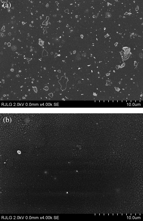
Field emission scanning electron microscopy SEIs of representative fields collected during Case 1: (a) collected with the ESP at the source; (b) collected with the TP at the BZ.

A series of images was taken at moderate magnification (×4000) on the sample in Fig. 5a and analyzed with IMAGEJ (Abramoff et al., 2004) to produce the complete size distribution shown in Fig. 6. This distribution matches reasonably well the EEPS and APS results. Particles in the 200–300 nm range were abundant on TEM grids collected at the source (illustrated in Fig. 5a) and were determined by EDS to be composed of Al. Note that the physical diameter (TEM), electrical mobility diameter (EEPS), and aerodynamic diameter (APS) may differ from each other.

Fig. 6.

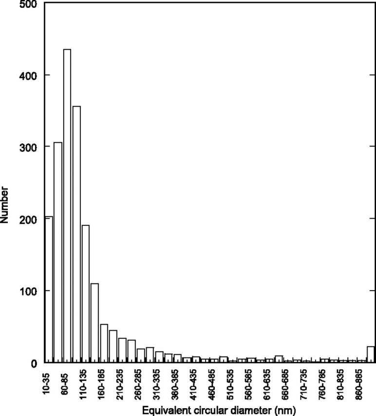
Particle size distribution obtained from the ESP (Case 1, source) presented in Fig. 5a.

Figures 7 and 8 present a variety of particles at the source and at the BZ from the same Case 1 (Al alloy 6061-T6) FSW process. In Fig. 7b, the EDS spectrum clearly shows the presence of Mg and Al, the two elements with the highest concentration in the Al 6061-T6 alloy. The particle morphology (Fig. 7a) suggests an agglomeration of smaller particles that appear to have melted or bonded together to form a larger (several hundred nanometers) particle. In fact, all the Al-bearing particles seen at the source and BZ appear to have a similar morphology but varying levels of Al, often with small amounts of other elements (Figs. 8g,h). Some larger particles (Fig. 8c,d) found on the source grids had higher Al content. This finding is important as it reconciles the large amounts of Al found on the upper WRASS stages.

Fig. 7.

Aluminum particles collected with ESP (Case 1, source): (a) Typical Al particle field emission scanning electron microscopy (FESEM) image; (b) EDS from (a) showing presence of major elements (Mg and Al) present in 6061-T6 aluminum. (c) FESEM image of a larger particle; (d) EDS from (c) showing high Al content.

Fig. 8.

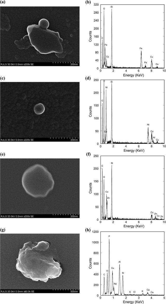
Particles collected with the ESP at the source and with the TP at the BZ for Case 1: (a and b) 60 nm diameter spherical Fe particle, from source, attached to a SiO² flake; (c and d) Ni particle, from source; (e and f) Zn particle, from BZ; (g and h) large Al particle, from BZ.

Smaller particles in both the source and the BZ sample grids appeared to have a spherical morphology and be comprised of pure metals, which support the ICP-MS data. Fig. 8 shows examples of Fe, Ni, and Zn particles. While the weld alloy contains trace amounts (<1% w) of these elements, as does the welding tool, the mechanism by which these pure element particles are formed has not been determined. The size and morphology suggest that localized heating above the expected temperatures may be occurring in the weld process, resulting in possible generation of metal fumes. This seems to be the most logical explanation for the large amounts of Zn particles in the nanoscale range.

Local exhaust ventilation efficacy

The FSW section of the laboratory is equipped with two arm-type fume extractors (snorkels) that are commonly used in welding facilities. Although these local exhaust ventilation (LEV) ducts are routinely used continuously during the welding process, they were turned off during our study to enable proper characterization of the source, as well as to enable estimation of potential BZ aerosol concentrations from operation of the FSW without the benefit of LEV. This also allowed for proper characterization of the collection efficiency of the LEV during the FSW operation. The intake of the LEV was positioned at an angle of ∼45°, almost resting on the mill table, and 10 cm from the welding location. When operating, the flow rate at the LEV intake was measured to be 5295 l min⁻¹ (187 cubic feet per minute). Case 1 was repeated four times with the LEV on, allowing each suite of instruments to collect two sets of measurements from both the BZ and the source. Using only data from the EEPS, the mean TNC for Case 1 was calculated from two and four measurements at each location for the LEV on and off, respectively. The mean TNC at the source was reduced by 99%, from 263 868 to 1990 particles cm⁻³ when the LEV was turned on. Similarly, the mean TNC at the BZ was reduced by 80%, from 9777 to 1871 particles cm⁻³ when the LEV was turned on. The mean total particle concentrations measured with the LEV on could not be distinguished from the background. Hence, the LEV inlet position and flow rate used were effective for reducing exposure to nanoparticles emitted by this FSW process.

DISCUSSION

Aerosol emission was directly related to the FSW weld, starting with a first peak after the tool touched the workpiece and ending with a second peak prior to tool retraction. The size distribution of particles was bimodal with peak maxima at ∼30 and 550 nm. Total particle number concentration as measured by EEPS (5.6–560 nm range) as high as 3.9 million particles cm⁻³ was measured 20 cm away from the source. Considerable spatial variability was noted, with the mean concentration at the BZ an order of magnitude lower than at the source. Peak exposures as high as 2.5 million particles cm⁻³ were recorded at the BZ, reflecting the transient nature of the process.

Exposure characteristic

The chemical composition of this aerosol determined by ICP-MS and verified by electron microscopy was made largely of Al, Fe, and Zn, with trace amounts of Ni, Cr, and Mn. All these elements originated largely from the workpiece, as expected, based on its chemical composition and the lack of signature elements (such as Mo) found only in the tool material. Although Mg was not quantitated by ICP-MS, its presence in substantial amounts in the Al alloy workpiece, confirmed by EM, suggests that Mg may have been present in quantifiable amounts (comparable to Fe, perhaps) in the emitted aerosol. Association of Al and Fe with the coarse aerosol (Table 5; Figs. 6, 8, and 9) suggests that the coarse particles may be generated through mechanical forces, whereas agglomeration of smaller particles may play a role in the low submicrometer fractions. An interesting finding relates to Zn, which was present in the sampled aerosol at much higher concentrations than one would expect from the chemical composition of the Al alloys (Al 92.5–98.6%; Zn ≤0.25%). The rich content of Zn in the low nanoscale size aerosol compared to the larger Al-rich particles suggests two possibly distinct mechanisms of its formation. Zn in large particles may result primarily from mechanical forces that eject small fragments of the Al alloy, a hypothesis apparently confirmed by electron microscopy and elemental EDS analysis of the grids collected at the BZ. Zn in nanoscale particles may be emitted as fumes resulting from localized melting of the Al alloy workpiece around the tool, a finding consistent with the process description and the fact that Zn has the lowest melting and boiling points of all metals in the Al alloy (e.g. 402 and 907°C, respectively, for Zn as compared to 660 and 2467°C for Al and 1811 and 2750°C for Fe).

Another possible source of Zn may be the lubricant used on the ways (i.e. table slides) of the mill used to carry out the FSW experiments. The material safety data sheet (MSDS) of the lubricant (Mobilith AW-2, Exxon Mobil Corp., Irving, TX) lists zinc dialkyl dithiophosphate as the main ingredient (1–5% w). The presence of other elements on EDS spectra, particularly S and P, and occasional observations of a ‘splatter’ pattern on the TEM grids further supports this as a possible explanation. The origin and mechanism of formation of spherical pure Fe particles are also not known.

Process characteristics

The current experiments studied two main factors: the Al alloy material and the rotation speed of the tool. No significant differences were seen among all cases at the source, though small differences may have been masked by variability in the data. More obvious differences are apparent at the BZ and are associated more prominently with the Al alloy 5083-H111, for which the higher r.p.m. speed resulted in higher particle number concentration than the lower r.p.m.. Also, larger particles were generated at the higher r.p.m. speed during FSW of this alloy. It is possible that FSW of other alloys requiring higher speeds may generate even higher exposures.

Instruments performance

Several instruments were employed in this study for the characterization of exposures during FSW, enabling evaluation of the most important physicochemical characteristics of exposures. The fast-response (1 s) instruments were essential in reliably capturing the size distributions of transient exposures on the order of 20 s, which cannot be done reliably with instruments with a slower scan time. The suite of instruments used also enabled collection of size distributions across a broad range of sizes, which, despite a focus on the nano-sized particles, was also important in this study. The size distribution was independently confirmed and reconstructed with electron microscopy imaging. Furthermore, the use of a size-selective sampler, such as the WRASS, not only confirmed the expected elemental composition of emitted aerosols but it more importantly provided an interesting perspective as to the source of the airborne Zn.

Another important aspect emerging from the employment of multiple instruments is the illustration of the key challenge in monitoring nanoscale particles—that is, traditional exposure metrics, such as total dust mass concentration or elemental mass concentration simply do not give a complete picture. Although the focus of this paper is not to compare instruments with each other, it is important to note the obvious correlation between EEPS, P-Trak, NSAM, and APS (Tables 3 and 4).

Since primary instruments, EEPS and APS, measure particle size by two different principles (electrical mobility versus aerodynamic diameter), it is important to know the extent to which these measurements may disagree. The size distribution reconstructed from the electron microscopy imagining matched reasonably well size distributions from EEPS and APS. The particle size maxima in Fig. 6 was 60–85 nm, about twice the peak maxima of ∼30 nm determined by EEPS. It is likely that this discrepancy may be a result of several factors, including particle agglomeration, which was well documented in this case, a bias in the fast mobility particle sizer (FMPS) measurements or imaging bias with smaller particles. Recent comparative work has shown that FMPS (which has the same hardware as EEPS) tends to underestimate the particle size in the sub-100 nm range compared to scanning mobility particle sizers (Asbach et al., 2009), which the authors confirmed with reference 100 nm polystyrene latex particles. In this same study, the FMPS response was different for NaCl and diesel exhaust aerosols. The FMPS distributions of NaCl aerosols were significantly broader than, whereas the count median diameters (CMDs) and the TNC were comparable to, scanning mobility particle sizers. The FMPS distributions for the diesel soot aerosols showed opposite trends than NaCl aerosols-narrower distributions, smaller CMDs, and higher total numbers. It is therefore possible that the EEPS in our study may have underestimated the particle size in the nano range. Park et al., (2008) found no relationship between the mobility diameter and aerodynamic diameter for the flame soot aerosols in the submicrometer range (200–700 nm) when using independent confirmatory techniques, raising serious doubts about the relationships (or lack thereof) between the EEPS-measured electrical mobility diameters and the desired aerodynamic diameter. No distinct peak maximum is apparent in the 0.3–0.8 μm in Fig. 6, although this may also be due to lower sensitivity of the size distribution reconstruction approach. For spherical particles made mostly of Al (specific gravity = 2.8), Zn (7.1), and Fe (7.8), the aerodynamic diameter would be ∼1.6 to 2.8 times higher than the physical diameter or electrical mobility diameter measured by EEPS. It is therefore quite possible that part of the dip in the merged size distributions may be caused by different principles of measuring particle size and the different collection efficiencies of the two instruments (EEPS and APS) at this size range. The EEPS-measured size distribution is likely to be shifted to the right if expressed as an equivalent aerodynamic diameter size distribution. The WRASS mass distribution data confirm the observed peak at ∼0.6 μm (aerodynamic diameter) to be almost entirely Al, whereas the major broad peak centered at 30 nm (mobility diameter) to be almost entirely Zn in the range of 2–60 nm aerodynamic diameter.

Control effectiveness

The FSW process investigated in this paper was conducted at a research laboratory and, being experimental in nature, it involved brief (<1 min) processes with transient exposure profiles. For the main study, the LEV was intentionally turned off to characterize process emissions and assess exposures under a ‘worst-case’ scenario. A few tests were conducted with LEV, resulting in particle measurements that were indistinguishable from the background. The interesting questions following the findings of this study are (i) What are the exposure levels during larger scale, continuous industrial FSW operations? (ii) Are there additional process conditions or factors that may moderate or increase exposures? (iii) To what degree are such exposures of concern to human health, especially in the long term? These questions require further investigation. Integrated daylong average BZ particulate concentrations were on the order of 10–30 μg m⁻³, whereas the estimated peak respirable particulate concentrations were ∼10 times higher (180–300 μg m⁻³). Similarly, the WRASS-derived estimates of the daylong average metal-specific concentrations were 2.0 (Zn), 1.4 (Al), and 0.24 (Fe) μg m⁻³ or lower. The estimated average peak metal concentrations were in a higher order of magnitude: 24, 17, and 3 μg m⁻³ for Zn, Al, and Fe, respectively. The WRASS-derived metal and personal respirable particulate exposure estimates agree reasonably well with the corrected DustTrak measurements. A comparison of FSW with traditional welding and with existing exposure standards will be the subject of another publication.

The complexities of this study highlight the need for and benefits of a multidisciplinary team effort. Several researchers (mechanical engineers, aerosol scientists, field occupational hygienists, microscopists, biostatisticians, risk communication, and policy researchers) from multiple institutions were involved—contributing the necessary instrumentation and expertise during planning and conducting of experiments, as well as analyzing and interpreting the data. The study would not have been possible without concerted efforts across multiple disciplines and without involvement of the several institutions.

CONCLUSIONS

This study documents for the first time emission of nanoscale and submicrometer particles during the FSW process and reports on their chemical composition and emission dynamics. Potential for substantial exposures to fine and ultrafine aerosol, especially to Al, Fe, and Zn, exist during FSW operations. Although the use of LEV controlled the aerosol emission effectively, the study results call for the need to investigate exposures during industrial scale FSW operations.

This study shows the importance of full characterization of materials, careful monitoring strategies, and a cross-disciplinary team effort to adequately understand environmental health and safety risks. The growing literature on nanoparticle toxicology and available exposure studies illustrate the need to measure key particulate parameters (especially size distribution, surface area, chemical composition, and morphology) and also that it is important to assess aerosol spatial and temporal variations using combinations of techniques and carefully planned monitoring strategies.

FUNDING

National Science Foundation through the Grant Opportunities for Academic Liaison with Industry Program (CMMI-0824879), the Nanoscale Science and Engineering Centers Program (DMR-0425880 and DMR-0425826), and National Science Foundation-supported shared facilities at the University of Wisconsin-Madison and University of Massachusetts Lowell; the National Institute for Occupational Safety and Health Training Grant Program (5T010H008424-04).

References

- Abramoff MD, Magelhaes PJ, Ram SJ. Image processing with Image. J Biophoton Int. 2004;11:36–42. [Google Scholar]
- Asbach C, Kaminski H, Fissan H, et al. Comparison of four mobility particle sizers with different time resolution for stationary expsoure measurements. J Nanopart Res. 2009;11:1593–609. [Google Scholar]
- Christner B, Hansen M, Skinner M, et al. Fourth International Symposium on Friction Stir Welding; 12–14 May 2003. Park City, Utah. Cambridge, UK: The Welding Institute Ltd; 2003a. Friction stir welding system development for thin-gauge aerospace structures. [Google Scholar]
- Christner B, McCoury J, Higgins S. Fourth International Symposium on Friction Stir Welding; 12–14 May 2003. Park City, Utah. Cambridge, UK: The Welding Institute Ltd; 2003b. Development and testing of friction stir welding (FSW) as a joining method for primary aircraft structure. [Google Scholar]
- Colegrove P. Airbus evaluates friction stir welding. COMSOL News. 2007:4–7. Available at: http://www.addlink.es/boletin/AGDWeb1512.pdf. [Google Scholar]
- Colligan KJ, Konkol PJ, Fisher JJ, et al. Friction stir welding demonstrated for combat vehicle construction. Weld J. 2003;82:34–40. [Google Scholar]
- Gorbunov B, Priest N, Muir R, et al. A novel size-selective airborne particle size fractionating instrument for health risk evaluation. Ann Occup Hyg. 2009;53:225–37. doi: 10.1093/annhyg/mep002. [DOI] [PMC free article] [PubMed] [Google Scholar]
- Halverson B, Hinrichs J, Smith C. Friction stir welding (FSW) of littoral combat ship deckhouse structure. Fort Lauderdale, FL: SNAME Maritime Technology Conference & Expo; 2006. [Google Scholar]
- Hoover MD, Stefanik AB, Day GA, et al. Chapter 5: exposure assessment considerations for nanoparticles in the workplace. In: Monteiro-Riviere NA, Tran CL, editors. Nanotoxicology characterization, dosing, and health effects. New York: Informa Healthcare; 2007. pp. 71–97. [Google Scholar]
- Kalle SW, Davenport J, Nicholas ED. Railway manufacturers implement friction stir welding. Weld J. 2002;81:47–50. [Google Scholar]
- Konkol PJ, Mathers JA, Johnson R, et al. Fourth International Symposium on Friction Stir Welding; 14–6 May 2003. Park City, Utah. Cambridge, UK: The Welding Institute Ltd; 2003. Friction stir welding of HSLA-65 steel for shipbuilding. [Google Scholar]
- Lienert TJ. Joining of advanced and specialty materials VI. Materials Park, OH: ASM International; 2004. Friction stir welding of DH-36 steel; pp. 28–34. [Google Scholar]
- Lienert TJ, Tang W, Hogeboom JA, et al. Fourth International Symposium on Friction Stir Welding; 14–6 May 2003. Park City, Utah. Cambridge, UK: The Welding Institute Ltd; 2003. Friction stir welding of DH-36 Steel. [Google Scholar]
- Miller C, Crawford MH, French R, et al. Welding-related expenditures, investments, and productivity measurement in U.S. manufacturing, construction, and mining industries. Miami, FL: American Welding Society; 2002. http://files.aws.org/research/HIM.pdf. Accessed 20 December 2009. [Google Scholar]
- Mishra RS, Ma ZY. Friction stir welding and processing. Mater Sci Eng. 2005;R50:1–78. [Google Scholar]
- Nishikawa H, Fujimoto M. Control of rotational distortion in friction stir welding. Weld World. 2004;48:79–85. [Google Scholar]
- Park K, Dutcher D, Emery M, et al. Tandem measurements of aerosol properties—a review of mobility techniques with extensions. Aerosol Sci Technol. 2008;42:801–16. [Google Scholar]
- Posada M, DeLoach J, Reynolds AP, et al. Fourth International Symposium on Friction Stir Welding; 14–6 May 2003. Park City, Utah. Cambridge, UK: The Welding Institute Ltd; 2003. Evaluation of friction stir welded HSLA-65. [Google Scholar]
- Przydatek JA. First International Symposium on Friction Stir Welding. Thousand Oaks, CA. Cambridge, UK: The Welding Institute Ltd; 1999. Ship classification view of friction stir welding. [Google Scholar]
- Schortt M. Friction stir welding emerges as high-performance alternative to fusion welding. Job Shop Technol. 2003:11–21. [Google Scholar]
- Smith CB. Robotic friction stir welding using a standard industrial robot. 2nd International Friction Stir Welding Symposium. Gothenburg, Sweden. 2000;2:1–10. Cambridge, UK: The Welding Institute Ltd. [Google Scholar]
- Smith CB, Crusan W, Hootman JR. Proceedings of the TMS—Aluminum Automotive and Joining Sessions. 2001. Friction stir welding in the automotive industry; pp. 175–85. Warrendale, PA: The Minerals, Metals & Materials Society. [Google Scholar]
- Smith CB. Friction stir weld market analysis. In: Pfefferkorn FE, editor. Waukesha, WI: 2008. [Google Scholar]
- Smith CB, Hinrichs JF, Crusan WA. Friction stir welding stirs up welding process competition. Forming Fabricating. 2003;10:25–31. [Google Scholar]
- Thomas WM, Nicholas ED, Needham JC, et al. Friction Welding. Cambridge, UK: The Welding Institute TWI; 1991. Patent Application No 91259788. [Google Scholar]