Automated volumetric evaluation of stereoscopic disc photography

Abstract

PURPOSE: To develop a fully automated algorithm (AP) to perform a volumetric measure of the optic disc using conventional stereoscopic optic nerve head (ONH) photographs, and to compare algorithm-produced parameters with manual photogrammetry (MP), scanning laser ophthalmoscope (SLO) and optical coherence tomography (OCT) measurements. METHODS: One hundred twenty-two stereoscopic optic disc photographs (61 subjects) were analyzed. Disc area, rim area, cup area, cup/disc area ratio, vertical cup/disc ratio, rim volume and cup volume were automatically computed by the algorithm. Latent variable measurement error models were used to assess measurement reproducibility for the four techniques. RESULTS: AP had better reproducibility for disc area and cup volume and worse reproducibility for cup/disc area ratio and vertical cup/disc ratio, when the measurements were compared to the MP, SLO and OCT methods. CONCLUSION: AP provides a useful technique for an objective quantitative assessment of 3D ONH structures.

1. Introduction

Glaucoma is the second most common cause of blindness in the world. Excavation of the optic nerve head (ONH) is a typical clinical sign of glaucoma. Disruption of the connective tissue support at the optic disc and posterior displacement or thinning of the lamina cribrosa may also play a morphological role in optic cup enlargement [1]. Regardless of the mechanism, accurate assessment of the optic disc is paramount in the routine clinical review of patients with ocular hypertension and glaucoma.

Optic disc imaging devices have an important clinical role, given the inherent difficulties in obtaining accurate measurements of the ONH at the slit lamp and the substantial inter-observer variability [2]. Stereoscopic disc photography has been used to document structural abnormalities and longitudinal changes in glaucomatous eyes for decades. It is the most common method for optic nerve head (ONH) imaging and is used for analysis and diagnosis [4]. In a previous publication we described a new method that allowed automated quantification of ONH structures using stereo photographs [3,4]. Further development of this method has enabled three-dimensional (3D) reconstruction of the ONH and quantification of structures, allowing volumetric quantification of the ONH from a widely available and low-cost imaging source. The advantages of this technique are: (1) objective quantitative measurements of conventional stereo photographs that are otherwise subjective and qualitative, (2) a cost-effective alternative to more sophisticated ocular imaging devices, such as confocal scanning laser ophthalmoscope (CSLO) and optical coherence tomography (OCT), and (3) a bridge between the old legacy data of stereo photographs, which have routinely been collected for clinical evaluation, and the newer technologies (CSLO and OCT).

The aims of this study were to describe a fully automated method for volumetric measurements of the ONH using a photogrammetric algorithm, to evaluate its performance in comparison with the measurements obtained from CSLO and OCT.

2. Methods

2.1 Study participants

Sixty-one consecutive subjects from the University of Pittsburgh Medical Center Eye Center were retrospectively enrolled in the study. Subjects were eligible for the study if they had refractive error within 6 diopters of emmetropia and no ocular pathologies other than those attributed to glaucoma. Both eyes of each subject were imaged, and presented with a wide range of clinically defined ONH characteristics ranging from healthy to advanced glaucoma. The study was approved by the Institutional Review Board (IRB) and adhered to the Declaration of Helsinki and Health Insurance Portability and Accountability Act Regulations. Written informed consent was obtained from each subject.

All subjects had a comprehensive ophthalmic evaluation, axial length measurement with the IOL master (Carl Zeiss Meditec, Dublin, CA), reliable visual field test (Humphrey Field Analyzer; Carl Zeiss Meditec, Dublin, CA; with less than 30% fixation losses, false-positive and false-negative responses), CSLO (Heidelberg Retina Tomograph (HRT) 3, Heidelberg Engineering, Heidelberg, Germany) and OCT (Stratus OCT; Carl Zeiss Meditec, Dublin, CA). Subjects’ pupils were dilated with 1% tropicamide and 2.5% phenylephrine (Alcon Laboratories, Fort Worth, TX) and stereoscopic disc photographs were obtained (Nidek 3Dx; Nidek, Gamagori, Japan). All tests were acquired within a six-month period.

2.2 Automated photogrammetry

Nidek 3Dx and a Nikon D1x digital camera unit (Nikon, Tokyo, Japan) was used for optic disc photography. The image resolution was 1312 × 2000 pixels. The stereo-pairs were cropped to 480 × 1020 pixels for image registration and 3D reconstruction. Image analysis and 3D modeling of the ONH were performed using software of our own design, as previously described [3,4]. A process flowchart was illustrated in Fig. 1 to give a short introduction of the designed software. A series of technical algorithms were developed to automatically generate ONH volumetric measurements based on conventional stereoscopic photographs. The process included: (1) 3D ONH reconstruction, (2) 2D and 3D magnification correction, (3) Optic disc and cup margin detection, and (4) Optic cup volumetric measurements. Enhancements to the previously described software added new functionality, specifically in step (2), (3) and (4).

Fig. 1.

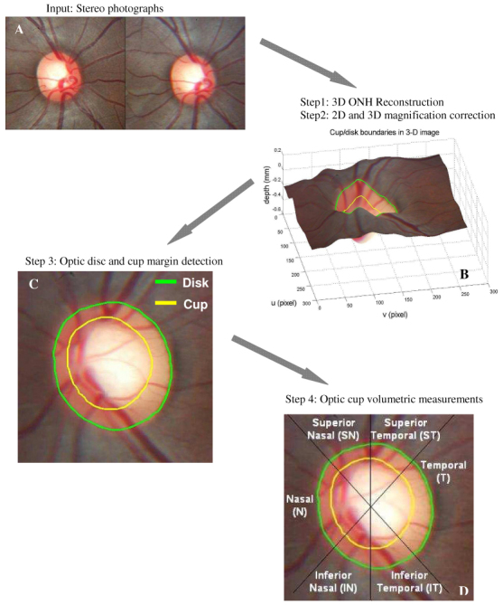
: Overview of the process flow

2.2.1 3D ONH reconstruction

In the stereo image pair, depth is inversely proportional to the disparity between the two matching points from the left and right images (Fig. 2 ), where the coordinate difference (v_L-v_R) of the corresponding points is defined as the disparity [3,4,15]. Multiple corresponding points were identified automatically on the left and right images by calculating the combination of the highest correlations and minimal differences of features within the given searching window. The disparities of the corresponding points were converted into depths. The scaled 3D ONH model was then generated from sparse corresponding points and interpolation (Fig. 1A,B).

Fig. 2.

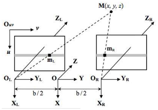
: Parallel stereo image configuration

2.2.2 2D and 3D magnification correction

The ocular media inside the eye had optical effect to the imaging system of the stereo fundus camera, therefore a scaled 3D ONH model was reconstructed from a pair of stereo images. Scaled estimates based on both the eye and the camera were calculated to correct the 3D depth as well as 2D image magnifications.(Fig. 3 ) Littmann’s formula [5] was applied to calculate the actual size of the image in 2D using axial length and camera specifications. 3D magnification correction was performed using the modified formula previously described by Xu and colleagues [3]:

$$\mathrm{\Delta }Zr=Zr-Z{r}_0=\mathrm{\Delta }Z\frac{2Z{r}_0{f}_e-f_e^2-Z{r}_0^2}{f_e^2-\mathrm{\Delta }Z{f}_e+\mathrm{\Delta }ZZ{r}_0}$$ (1)

$f_e$ was the focal length of the simplified imaging model of the eye. Any arbitrary reference plane could be used to compute relative depth. The plane generated from the ONH margin was set to be the reference plane $Z{r}_0$ in this study. $Z{r}_0$ was the location of the reference plane to the optical center of the simplified imaging model of the eye, $Zr$ was the ONH pixel location, $\mathrm{\Delta }Z$ was ONH depth from the reference plane $Z_0$ on scaled virtual 3D model, and $\mathrm{\Delta }Zr$ was the converted true depth of ONH. In the previous iteration of the software the maximal depth was obtained with HRT to compute $Z{r}_0$. In the current version of the software the axial length was used to compute $Z{r}_0$ in order to generate the actual depth from the scaled virtual 3D disc model.

Fig. 3.

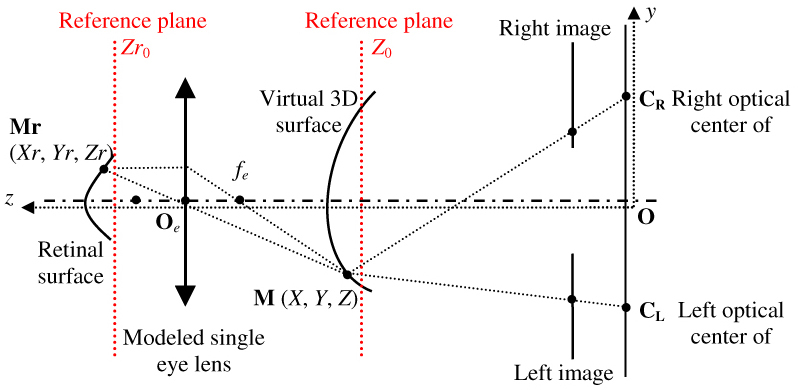
Optical model of the eye and stereo fundus camera (adapted from Deguchi’s [15]).

2.2.3 Optic disc and cup margin detection

The geometrical center of the region with the highest intensity value on the image was located as the disc center. The disc margin was generated using a deformable model technique whereby a smooth boundary of high contrast surrounding the disc center was detected (Fig. 1C). The image features, such as pixel intensity value, gradient, and contour smoothness, were extracted and used in computation of the deformable model [6]. The cup was located at 150μm posterior to the disc margin for eyes where 0.2mm ≤ cup depth ≤ 1.0mm, or at the 1/5 depth from the disc margin to the deepest point of the cup for eyes with cupping < 0.2mm or > 1.0mm (Fig. 4A ). Cup margin was extracted using a deformable model technique similar to that described for disc margin detection; however, a different energy function, which amalgamated data relating to cup depth and location, intensity gradient, contour smoothness and shape, was used. Optic cups were assumed to be located in close proximity to the geometrical center of the optic disc to control the flexibility of the deformable model and avoid generating the cup margin of irregular shape.

Fig. 4.

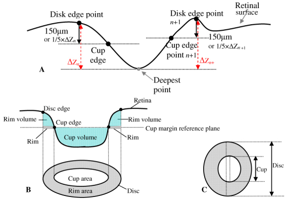
: Geometric model of optic nerve head (ONH) with cross sectional profile and projected image. (A) Locating cup margin points in deformable model algorithm. (B) Cross sectional profile of 3D ONH model, with definitions of various ONH parameters, i.e., disc area, rim area, cup area, rim volume and cup volume. (C) The definitions of vertical C/D ratio and C/D area ratio.

2.2.4 Optic cup volumetric measurements

Magnification corrections were applied on each stereo disc photograph as described in step (2) to compute the 3D and 2D scales and to generate the actual size 3D disc model. Seven ONH parameters, disc area, rim area, cup area, cup-to-disc (C/D) area ratio and vertical C/D ratio, were automatically generated by the designed software (Fig. 4B,C). Disc area and cup area were defined as the area inside the disc margin and cup margin respectively, while rim area was defined as the area inside the disc margin but outside cup margin. C/D area ratio was the cup area divided by disc area. Vertical C/D ratio was defined as the vertical cup diameter through the geometric center divided by the vertical disc diameter through disc center (Fig. 4C). All the areas and ratios were measured on the 2D stereo disc photograph. A 3D reference plane was generated from the detected cup margin on the 3D disc model, as illustrated by the cross sectional profile in Fig. 4B. The voxel size was computed from the corrected 3D disc model. The cup volume was measured as the summation of the total number of voxels within the disc margin and below the reference plane multiplied by the voxel size, while rim volume was the voxels within the disc margin between the reference plane and the 3D optic disc surface (Fig. 4B).

2.3 Quality assessment of the automatically detected disc margin

The developed software provided a fully automated ONH assessment. Detected disc margin quality was assessed by an independent and automated method using Fourier transform analysis. The disc margin was converted in polar coordinates centered at the geometric center of the detected disc margin and then transformed into Fourier domain. Automated quality assessment was used by analyzing the frequency along the margin in Fourier domain. The assumption is that optic disc is close to oval shape with a smooth boundary. High frequency components correspond to noise on the boundary. Therefore the boundary with an unsmooth and irregular shape should have more high frequency components and is more like to be a failure. The analysis was defined as successful when the low frequency energy was larger than 87.5% (7/8) of the total energy and the high frequency energy was less than 5%. Low frequency was defined as < 7% of the frequency components at the lower end, and high frequency was defined as the higher half of the frequency component. These thresholds were set arbitrarily.

2.4 Manual photogrammetry

Three glaucoma specialists independently and manually defined the disc margin and the cup margin on stereo disc photographs in a randomized and masked fashion. The final location of the disc and cup margins for the analysis was defined by the majority opinion of the observers using the method described by Abramoff et al. [7] Optic disc parameters were generated from the manual disc demarcation using the same processes of 3D modeling and 2D and 3D magnification correction methods as those described above for the automated photogrammetry.

2.5 HRT

HRT scans were performed using a HRT2 device. The files were then transferred to HRT3 software to be processed. Eligible images had pixel standard deviation < 50µm with even illumination, acceptable centration and focus. The optic disc margin was manually delineated at the border of Elschnig’s ring and the disc parameters were generated by the HRT3 software (version 1.5.10.0).

2.6 OCT

Fast ONH scans were taken using Stratus OCT for each eye. Eligible images had signal strength > 7. The disc margin was automatically defined at the termination of the retinal pigment epithelium (RPE) in each of 6 radially sampled cross-sectional retinal images. The OCT software generated a disc margin by interpolating these 12 detected points. Manual correction were required if the disc margin was not correctly placed at the end of RPE. The disc parameters were then calculated by the OCT software (version 4.0.7).

2.7 Statistical analysis

Seven disc parameters including disc area, rim area, cup area, cup/disc area ratio, vertical cup/disc ratio, rim volume and cup volume were generated by the automated photogrammetric algorithm (AP), manual photogrammetry (MP) for each individual observer and the major opinion of the three observers, HRT and OCT. Latent variable measurement error models (LVM) were used to determine the relative biases (the relative systematic error for each technique) and imprecision (random error) for each method. LVM is a statistical method that extracts the shared properties among different parameters that aim to measure the same feature. The model requires that data from both eyes of the same subjects will be used. Both eyes were eliminated from this analysis if only one eye was qualified. A separate LVM was calculated for each of the seven parameters accounting for the correlation between eyes from the same subject. Square root transformation of the measurements was used to reduce positive skewness (lack of Normality) where necessary. In order to assess the difference in relative bias and imprecision between methods the ratio of the estimates was computed. The relative bias indicates whether the measurement from one method is consistently higher (bias ratio > 1) or lower (bias ratio < 1) than another method. Imprecision ratios were adjusted by taking imprecision standard deviation over bias. Higher imprecision SD corresponds to larger random error and lower reproducibility. If the ratio of imprecision SD between method A and B is less than 1, this indicates method A has better reproducibility than method B, and vice versa.

Linear calibration curves were computed (using the relative biases) and combined with estimates of imprecision to evaluate the relationship among the measurements of each method. Automated photogrammetry was used as the reference slope with all other methods calibrated accordingly. Mixed effect models were used to evaluate the differences in cases where there was a constant bias between the measurements. No statistical method is available to assess the difference in the presence of non-constant bias because the difference changes with level - i.e., measurements of MP is bigger than AP for bigger rim area values and smaller than AP for smaller rim area values.

The general statistical modeling software package Mx was used to estimate the LVM parameters [8]. Other statistical analyses were performed using the R Language and Environment for Statistical Computing (R 2.6.0, R development Core Team, 2007, http://www.r-project.org). P < 0.05 was considered as statistically significant.

3. Results

The mean age of the 61 participants in the study was 56.8 ± 9.6. Twenty-nine eyes (22 subjects) out of the 122 eyes (23.8%) were labeled as no-success by the automated quality assessment of AP. Examples of algorithm success and failure appear in Fig. 5 .

Fig. 5.

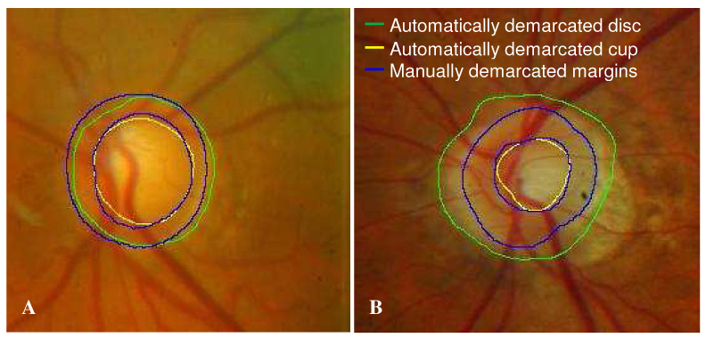
Comparison between automatically photogrammetric algorithm and manual disc demarcation. (A) A successful example of disc demarcation. (B) An example of failure in disc demarcation due to prominent peripapillary atrophy.

No consistent pattern in terms of mean and standard deviation was noted among the observers when the results obtained from each of the three individual observers were compared, i. e., comparing seven ONH measurements of one observer with measurements of majority opinion of three individual observers, some measurements were larger and others were smaller. For all ONH parameters, the correlation between the latent variables (representing the “true values”) between eyes of the same subject exceeded 0.93 (except for cup volume with a correlation of 0.79) indicating high correlation between eyes. Table 1 summarizes the mean and standard deviation of seven disc parameters measured by the four methods from all qualified eyes (78 eyes, 39 subjects). For most parameters there were non-constant biases so that the bias between methods depended on the level of the parameter. All parameters that had constant bias were statistically significantly lower than AP.

Table 1. : Comparison of optic disc measurements (mean ± standard deviation) from automated photogrammetry (AP), manual photogrammetry (MP), Heidelberg retina tomography (HRT) and optical coherence tomography (OCT).

	AP	MP	HRT	OCT
Disc area (mm2)	2.61 ± 0.58	2.53 ± 0.58*	2.10 ± 0.51*	2.47 ± 0.63*
Rim area (mm2)	1.59 ± 0.45	1.56 ± 0.39	1.31 ± 0.34*	1.46 ± 0.48
Cup area (mm2)	1.02 ± 0.53	0.97 ± 0.49	0.79 ± 0.52*	1.02 ± 0.68
Cup/disc area ratio	0.38 ± 0.15	0.37 ± 0.14	0.36 ± 0.18	0.39 ± 0.21
Vertical cup/disc ratio	0.62 ± 0.12	0.61 ± 0.12	0.57 ± 0.16	0.58 ± 0.17
Rim volume (mm3)	0.23 ± 0.15	0.25 ± 0.14	0.33 ± 0.15	0.34 ± 0.25
Cup volume (mm3)	0.28 ± 0.28	0.26 ± 0.23	0.21 ± 0.19	0.20 ± 0.19*

*Comparison with automated photogrammetry was computed only for parameters with constant bias. For all these parameters a statistically significant (p < 0.05) difference was noted.

Table 2 summarizes the imprecision standard deviation (SD) for each method. Table 3 summarizes the imprecision ratio (adjusted by bias) among the methods. Disc area measurements obtained by MP had a SD that was 2.0054 times larger than those obtained with AP (Table 3). As the confidence interval did not cross the value of 1, this ratio was statistically significant. MP had the smallest SD among the four methods for most of the disc parameters. The imprecision SDs of the AP were statistically significantly lower for disc area, rim volume and cup volume (except for rim volume comparison between AP and MP that did not reach statistically significant level), and the highest for rim area, cup area, cup/disc area ratio and vertical cup/disc ratio (although cup area comparisons between AP and the other three methods, and rim area comparisons between AP and both HRT and OCT did not reach the statistically significant level), compared with MP, HRT and OCT. This indicates that AP had statistically significantly smaller variability (lower SD) in measuring disc area, rim volume and cup volume. When the comparison was conducted between AP and each individual observer’s measurements, there were inconsistent results with any of the observers or the AP showing alternately the best performance.

Table 2. Imprecision standard deviation of optic disc parameters measured by automated photogrammetry (AP), manual photogrammetry (MP), Heidelberg retina tomography (HRT) and optical coherence tomography (OCT).

	AP	MP	HRT	OCT
Disc area (mm2)	0.1321	0.2463	0.2847	0.3569
Rim area (mm2)	0.1572	0.0493	0.1267	0.2029
Cup area (mm2)	0.2400	0.2165	0.1754	0.1940
Cup/disc area ratio	0.1070	0.0474	0.0751	0.0905
Vertical cup/disc ratio	0.1021	0.0350	0.1062	0.0947
Rim volume (mm3)	0.1164	0.1093	0.1490	0.2724
Cup volume (mm3)	0.0752	0.1433	0.1285	0.1097

Table 3. Relative imprecision standard deviation ratio (adjusted by bias, 95% confidence interval) of optic disc parameters measured by automated photogrammetry (AP), manual photogrammetry (MP), Heidelberg retina tomography (HRT) and optical coherence tomography (OCT).

	MP/AP	HRT/AP	OCT/AP
Disc area (mm2)	2.0054* [1.4364, 2.7826]	2.8082* [2.0485, N/A]	2.9363* [2.1114, N/A]
Rim area (mm2)	0.1164* [0.0153, 0.4121]	0.4610 [0.0049, N/A]	0.7878 [0.0003, N/A]
Cup area (mm2)	0.9793 [0.7119, N/A]	0.7018 [0.5193, 0.7018]	0.5041 [0.4285, N/A]
Cup/disc area ratio	0.3718* [0.2250, 0.5978]	0.5119* [0.3173, 0.8039]	0.4507* [0.2778, 0.7088]
Vertical cup/disc ratio	0.2189* [0.1715, 0.3155]	0.6027* [0.3542, 0.8765]	0.4790* [0.5559 1.1572]
Rim volume (mm3)	1.9669 [0.9819, 5.2616]	15.6618* [2.6423, N/A]	8.8209* [2.2745, N/A]
Cup volume (mm3)	2.6641* [1.9456, N/A]	2.4498* [1.7998, 3.4187]	1.8050* [1.3424, 2.4529]

*P < 0.05. N/A – value did not converge.

The slopes (relative bias ratio) and intercepts of the calibration curves are given in Table 4 and Fig. 6 . No constant bias was apparent for most measurements among the four methods, as shown in Fig. 6, with calibration curves intersect each other. For example, disc area measurements obtained by MP increased 6.98% (1-0.9302) slower than disc area measurements that were obtained by AP (Fig. 6A). Disc area, rim area and cup area obtained by AP were constantly (no cross point) and statistically significantly higher than HRT measurements, while disc area and cup volume were statistically significantly higher with AP than OCT measurements. The differences in the calibration curves between AP and MP tended to be smaller compared to the differences with HRT and OCT in all ONH measurements.

Table 4. Linear calibration between optic nerve head measurements of automated photogrammetry (AP), manual photogrammetry (MP), HRT and OCT. AP was set as reference and all measurements were accordingly adjusted.

	MP vs AP		HRT vs AP		OCT vs AP
	slope	intercept	slope	intercept	slope	intercept
Disc area (mm2)	0.9302	0.1022	0.7678*	0.0980	0.9203	0.0674
Rim area (mm2)	1.5558	−0.9156	0.8221	0.0024	1.3465	−0.6810
Cup area (mm2)	0.9213	0.0317	1.0415	−0.2688	1.3843*	−0.3920
Cup/disc area ratio	1.1918	−0.0813	1.3700	−0.1661	1.8753*	−0.3237
Vertical cup/disc ratio	1.5807*	−0.3777	1.8066*	−0.5502	2.0120*	−0.6725
Rim volume (mm3)	0.4776*	0.1426	0.0817*	0.3128	0.2653*	0.2768
Cup volume (mm3)	0.7156*	0.0539	0.6979*	0.0140	0.8084*	−0.0325

*P < 0.05.

Fig. 6.

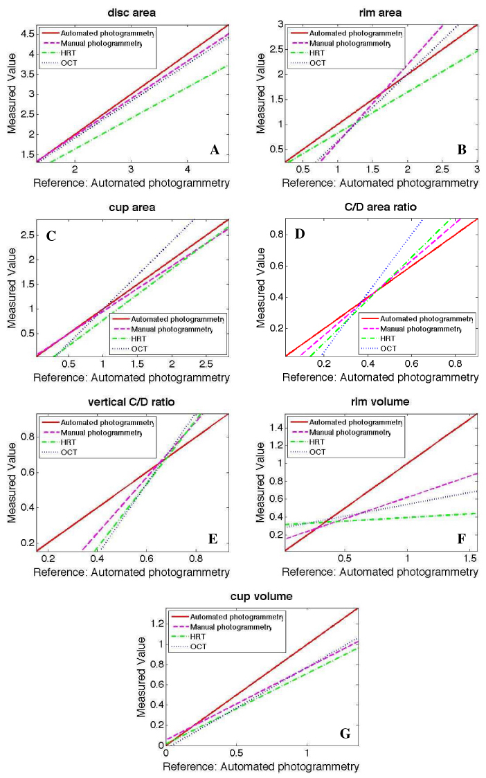
Relative bias comparison between optic nerve head measurements of automated photogrammetry, manual photogrammetry, Heidelberg retina tomography (HRT) and optical coherence tomography (OCT). Automated photogrammetry was used as reference to all other methods

4. Discussion

In this study we described an automated ONH photogrammetry technique that provided volumetric parameters (Fig. 1). ONH measurements from the new technique were compared with manual demarcation of the margins from three observers, major opinion of the three observers (MP), HRT and OCT. AP and MP showed high similarity as indicated by the mean and standard deviation values of the seven disc parameters (Table 1) and similar reproducibility to those obtained by the other automated imaging methods (HRT, OCT) (Tables 2, 3). Linear calibration equations were also computed to determine the relationship between measurements obtained by the various methods (Table 4 and Fig. 6).

An automated segmentation algorithm was used to demarcate the optic disc margin based primarily on the components of pixel intensity values, smoothness, and gradient in the image. We found however, that this automated method occasionally placed some disc margins away from the true location. This is likely due to indiscernible differences between Elschnig’s rim and peripapillary tissue in photographs (Fig. 5B).

The extraction or delineation of the optic cup margin is the initial requirement for the automated measurement of disc parameters. 3D depth information has been shown to be a reliable feature by which to segment the cup and as such many definitions for the optic cup have been proposed [9–13]. The HRT software defines the optic cup to be 50μm below the mean surface height along a six degree annulus at the temporal inferior disc margin [9]. OCT software defines the optic cup below a reference plane located 150μm superior to the RPE/Bruch’s membrane tips. In the automated program we used a hybrid approach where the cup margin was located at a fixed distance from the disc margin for average size cups, and a relative distance for large and small cups [4].

Non-constant bias was noted for most measurements between the methods indicating a difference that changes with the measurement level. Hence, measurements from one method could not simply be substituted by measurements from the other method plus or minus a certain value. In addition, although the linear calibration equation provided a way to adjust the systematic bias from one method to the other, the imprecision of the given method could not be replaced by the other method. Therefore, measurements are not inter-changeable between modalities. AP showed measurements similar to MP and was different from HRT and OCT. The difference, which was noted in cases where the comparison could be computed, might originate from the definitions of disc margin used by the different methods. OCT defines the ONH margin as the termination of the RPE (or Bruch’s membrane) in six radial scans. AP and HRT define the ONH margin as the high contrast edge points in the two-dimensional pseudo fundus photo images. However, disc photography, HRT and OCT used different wavelengths for light sources and different scanning principles, resulting in different anatomical locations as ONH margins [14].

The SD of disc area and cup volume with AP was statistically significantly smaller than with other three methods, indicating that AP of automated ONH margin detection and cup volume assessment provide more reproducible measurements, while cup/disc ratio measurements are more reproducible with the other three methods (Tables 2 and 3). The reason may be that all the other parameters are absolute values, while C/D area ratio and vertical C/D ratio are relative values. The relative value, such as vertical C/D ratio, is more sensitive to the exact locations and shape of the cup. It should be noted that manual intervention was present in all methods except for the AP, which might artificially affect the variability.

The limitation of this study was the substantial failure rate of the AP method (23.8%). This was due to the rigorous quality criteria that were employed for AP. The main causes for the failures were the presence of pathologic features such as peripapillary atrophy, which reduced the visibility of disc margin. It should be noted that all other methods used subjective input for their disc margin definition, which is also a viable option in cases where AP fails. Another limitation of the study was the use of stereo photographs that were acquired with the Nidek 3-DX camera only. However, minor modifications in the algorithm accounting for the specific properties of different cameras can be employed thus expanding the generalisability of this method. A small test sample obtained using another camera showed similar performance as those reported in this manuscript (unpublished preliminary data).

In summary, we present a photogrammetric method that provides a fully automated and objective volumetric quantification of the ONH. The method was comparable to other conventionally accepted methods of automated ONH analysis in term of measurement bias and imprecision although the measurements are not inter-changeable between modalities.