

Abstract
We analyze published auditory-nerve and otoacoustic measurements in chinchilla to test a network of hypothesized relationships between cochlear tuning, cochlear traveling-wave delay, and stimulus-frequency otoacoustic emissions (SFOAEs). We find that the physiological data generally corroborate the network of relationships, including predictions from filter theory and the coherent-reflection model of OAE generation, at locations throughout the cochlea. The results support the use of otoacoustic emissions as noninvasive probes of cochlear tuning. Developing this application, we find that tuning ratios—defined as the ratio of tuning sharpness to SFOAE phase-gradient delay in periods—have a nearly species-invariant form in cat, guinea pig, and chinchilla. Analysis of the tuning ratios identifies a species-dependent parameter that locates a transition between “apical-like” and “basal-like” behavior involving multiple aspects of cochlear physiology. Approximate invariance of the tuning ratio allows determination of cochlear tuning from SFOAE delays. We quantify the procedure and show that otoacoustic estimates of chinchilla cochlear tuning match direct measures obtained from the auditory nerve. By assuming that invariance of the tuning ratio extends to humans, we derive new otoacoustic estimates of human cochlear tuning that remain mutually consistent with independent behavioral measurements obtained using different rationales, methodologies, and analysis procedures. The results confirm that at any given characteristic frequency (CF) human cochlear tuning appears sharper than that in the other animals studied, but varies similarly with CF. We show, however, that the exceptionality of human tuning can be exaggerated by the ways in which species are conventionally compared, which take no account of evident differences between the base and apex of the cochlea. Finally, our estimates of human tuning suggest that the spatial spread of excitation of a pure tone along the human basilar membrane is comparable to that in other common laboratory animals.
Keywords: cochlea, frequency selectivity, auditory nerve, basilar membrane, otoacoustic emissions, psychophysical masking, filter theory, coherent reflection, model
Introduction
The cochlea transduces acoustic signals into an electrochemical form suitable for interpretation by the brain. A fundamental feature of the transduction process is the mechanical separation of the various frequency components in sound so that they stimulate different populations of sensory cells. The frequency analysis performed by the cochlea plays a critical role in the encoding of acoustic information by auditory neurons and, subsequently, in our ability to distinguish and segregate different sounds. Despite the perceptual significance of this filtering—and notwithstanding the wealth of information now available about the cellular, molecular, and genetic mechanisms of hearing—much remains unknown about this and other primary aspects of human peripheral auditory function. For example, even the tuning bandwidths of human cochlear filters, and how they vary with frequency, remain uncertain.
The problem is that in humans and other animals for whom direct measurements of mechanical or neural tuning are difficult or impossible to obtain, the characteristics of cochlear tuning must be measured noninvasively. The traditional approach relies on behavioral measurements involving paradigms such as psychophysical tuning curves (e.g., Moore 1978) or notched-noise masking experiments (e.g., Patterson 1976). In a previous paper, we proposed a method for using otoacoustic emissions to estimate the sharpness and frequency dependence of cochlear tuning (Shera et al. 2002). The method exploited an empirical correlation discovered in laboratory animals between physiological measurements of tuning in auditory-nerve fibers (ANFs) and the group delays of stimulus-frequency otoacoustic emissions. Applying the method to humans, we obtained estimates of tuning that differed substantially from conventional behavioral values (e.g., Glasberg and Moore 1990)—our estimates were sharper and varied more rapidly with frequency—but agreed well with values obtained using psychophysical procedures designed to resemble more closely the conditions under which ANF tuning curves are actually derived (Oxenham and Shera 2003).
A triangle of relationships
Our exploration of possible correlations between cochlear tuning and otoacoustic emissions was motivated by a broader network of hypothesized relationships whose principal elements can be represented by a triangle. In the schematic of Figure 1, three different aspects of cochlear physiology—cochlear tuning, cochlear delay, and otoacoustic emission delay—form the vertices of a triangle whose sides represent possible theoretical or empirical relationships linking the different domains. If quantitative relationships such as these were to prove valid and robust, measurements at one vertex would provide information about the others. For example, noninvasive measurements of otoacoustic emissions might be used to infer the sharpness and delay of cochlear tuning. Although the conceptual framework represented by the triangle raises intriguing possibilities, the nature and existence of the proposed relationships remain controversial. Indeed, in a series of recent papers, Ruggero and colleagues have questioned many aspects of the framework (Ruggero and Temchin 2007; Siegel et al. 2005), as well as its application to the determination of human cochlear tuning (Ruggero and Temchin 2005).
FIG. 1.

Triangle of hypothesized relationships linking otoacoustic emissions to cochlear mechanics and peripheral auditory tuning.
In this paper, we test the validity of the framework in chinchilla by using published measurements of auditory-nerve-fiber Wiener kernels (Recio-Spinoso et al. 2005; Temchin et al. 2005) and stimulus-frequency otoacoustic emissions (Siegel et al. 2005) to evaluate all hypothesized relationships throughout the cochlea. Broadly speaking, the paper has two parts. In the first part (Results), we proceed systematically around the triangle, first outlining the theoretical and/or empirical basis for the predicted relationships and then evaluating the relationships using neural and acoustic measurements in the chinchilla. In the second part (Applications), we show how the framework can be applied to estimate the sharpness of cochlear tuning from otoacoustic measurements. We illustrate the method—a revision and extension of that proposed earlier (Shera et al. 2002)—by validating otoacoustic estimates of chinchilla cochlear tuning using direct measurements from auditory-nerve fibers (Recio-Spinoso et al. 2005). We then apply the revised procedure to humans and demonstrate that otoacoustic estimates of human tuning agree with independent values derived from psychophysical masking experiments (Oxenham and Shera 2003). Finally, in the Discussion, we respond to published criticisms of our approach and speculate about the origin of the apparent differences in tuning between humans and common laboratory models of mammalian hearing (e.g., cats, guinea pigs, chinchillas).
Methods
General methods for Results
Our evaluation of the triangle of relationships relies on published measurements of auditory-nerve tuning and otoacoustic emissions in chinchilla (Recio-Spinoso et al. 2005; Siegel et al. 2005; Temchin et al. 2005). Figure 2 shows a handful of these measurements to highlight the types of information they provide. Panel A plots Wiener-kernel estimates of the amplitude and phase of near-threshold cochlear tuning at seven different locations spanning the length of the chinchilla cochlea (Recio-Spinoso et al. 2005). The Wiener-kernel method estimates cochlear tuning by extracting high-frequency timing information encoded in the neural response envelope by cochlear nonlinearities, principally the half-wave rectification that occurs at the inner hair cell synapse (e.g., Eggermont 1993). When corrected for synaptic and neural transmission delays, the Wiener-kernel estimates closely resemble mechanical measurements made on the basilar membrane (BM) at corresponding locations and intensities (Temchin et al. 2005). In addition to providing estimates of tuning bandwidth throughout the cochlea, the Wiener-kernel measurements allow determination of cochlear delays (e.g., from the slopes of phase-vs-frequency functions). Although we sometimes refer to the neural measurements as “BM responses” for convenience, the Wiener-kernel measurements characterize cochlear tuning as seen from the auditory nerve. They therefore presumably include contributions from internal motions of the organ of Corti or tectorial membrane visible to the inner hair cell but perhaps less prominent in the motion of the BM itself.
FIG. 2.

Example neural and otoacoustic measurements in chinchilla. Panel (A) shows the magnitude and phase of seven representative second-order Wiener kernels derived from responses to near-threshold noise in auditory-nerve fibers with characteristic frequencies (CFs) spanning the range of chinchilla hearing (Recio-Spinoso et al. 2005; Temchin et al. 2005). The magnitudes are normalized to the same peak value. Panel (B) shows chinchilla SFOAE magnitude and phase measured at a probe level of 30 dB SPL in five different ears (Siegel et al. 2005). The measurement noise floor averaged about −25 dB SPL (see figure 4 of Siegel et al. 2005). To facilitate visual comparison of phase gradients, the horizontal and vertical scale bars in the two panels are equal.
Otoacoustic measurements relevant to the triangle are shown in Figure 2B. As illustrated by the five examples in the figure, chinchilla stimulus-frequency otoacoustic emissions (SFOAEs) measured at low stimulus intensities display all the characteristic features of mammalian SFOAEs, including an amplitude spectrum punctuated by sharp notches and a rapidly rotating phase (Siegel et al. 2005). Of primary interest here are the slopes of SFOAE phase-vs-frequency functions, which provide measurements of otoacoustic delay. Taken together, the Wiener-kernel and SFOAE measurements exemplified by the data in Figure 2 provide information about each vertex of the triangle of hypothesized relationships at frequencies spanning almost the entire range of chinchilla hearing.
General methods for Applications
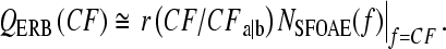
Our approach to applying the triangle to estimate cochlear tuning from otoacoustic measurements is fundamentally comparative. The procedure relies on published neural, otoacoustic, and behavioral data from a variety of common laboratory models of mammalian hearing (cats, guinea pigs, chinchillas, and humans). We quantified the sharpness of cochlear tuning using the QERB, defined as CF/ERB, where CF is the center or characteristic frequency and ERB is the equivalent rectangular bandwidth, a parameter-free measure of tuning bandwidth commonly adopted in the psychophysical literature. For any filter, the ERB is the bandwidth of the rectangular filter with the same peak response that passes the same total power when driven by white noise. Neural values of QERB were computed using standard algorithms (Evans and Wilson 1973) from threshold frequency tuning curves of single auditory-nerve fibers (Tsuji and Liberman 1997; Cedolin and Delgutte 2005) and from the chinchilla Wiener kernels previously described (Recio-Spinoso et al. 2005). Behavioral ERBs in humans were taken from our previous study (Oxenham and Shera 2003), where they were measured using notched-noise masking (Patterson 1976) with a paradigm designed both to limit the effects of nonlinear compression and suppression and to mimic more closely the procedures used in the measurement of neural tuning curves. Briefly, these procedures included the use of (1) signal levels near absolute threshold, to minimize compression and “off-frequency listening”; (2) non-simultaneous masking, to minimize suppressive interactions between the masker and the signal (Houtgast 1973); and (3) constant signal level rather than constant masker level, to mimic the constant-response paradigm used in neural threshold measurements (e.g., Rosen et al. 1998; Glasberg and Moore 2000). Cochlear filter shapes were derived from the individual and mean data using the roex(pwt) model and assorted variants (e.g., Patterson et al. 1982; Glasberg et al. 1984; Rosen et al. 1998; Glasberg and Moore 2000). Details of the experimental and analysis procedures are described elsewhere (Oxenham and Shera 2003).
We computed otoacoustic phase-gradient delays from unwrapped SFOAE phase-vs-frequency functions (Shera and Guinan 2003). In each of the four species, the SFOAE data (all previously published) were obtained using the acoustic and/or efferent suppression method (Guinan 1986; Dreisbach et al. 1998; Shera and Guinan 2003; Siegel et al. 2005) at low to moderate sound levels (30–40 dB SPL). For comparison with the dimensionless QERB, phase-gradient delays were expressed as the equivalent number, NSFOAE, of stimulus periods.
Results: testing the triangle of relationships
Relation between cochlear tuning and cochlear delay
Prediction from filter theory
Relationships between tuning and group delay are expected from filter theory, with sharper tuning generally requiring proportionally longer delay (e.g., Bode 1945). Figure 3 illustrates the covariation of tuning and delay using the frequency responses of a collection of masses on springs with different resonant frequencies and quality factors. The sharpness of tuning has been chosen to vary systematically with center frequency, just as it does in the mammalian cochlea. When the system is driven sinusoidally, the displacement of each mass relative to that of the drive (i.e., the ratio Yn/X in the figure, with n = 1,…,4) defines a filter whose magnitude has the resonant-like form shown in the top panel. The displacement ratios |Yn/X | approach one at low frequencies and reach a maximum when driven at frequencies near the undamped resonant frequencies of the oscillators, f0(n). The values 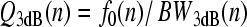 , where BW3dB(n) is the filter bandwidth 3 dB below the peak, quantify the sharpness of tuning. Increasing the quality factors of the resonators (moving left to right from n = 1 to n = 4 in the figure) boosts the height of the peak, which is approximately Q3dB, and sharpens the tuning.
FIG. 3.

Covariation of tuning and delay in a set of driven harmonic oscillators (second-order filters) with different resonant frequencies and quality factors. The figure shows the magnitudes (top) and phases (bottom) of the displacement ratios Yn/X versus driving frequency for four damped harmonic oscillators (e.g., masses on springs moving in a viscous medium). The in vacuo resonant frequencies are f0(n) = {1,2,4,8} kHz for oscillators n = {1,2,3,4}, respectively. Values of Q3dB (the sharpness of the magnitude peak) or N (the near-peak phase-gradient delay in stimulus periods) are given adjacent to each curve.
The bottom panel shows the corresponding filter phases, which transition from in-phase to out-of-phase behavior in frequency bands centered about f0(n). The center-frequency group (or phase-gradient) delay, given by the negative slope of the phase-vs-frequency function evaluated at the magnitude peak, provides a measure of the filter delay (e.g., Papoulis 1962). Expressing the delay not in seconds, but as the equivalent number, N, of periods of the resonant frequency, allows for easy comparison with the dimensionless Q3dB. The figure shows that lowering the value of Q3dB decreases the delay by the same proportion, with N(n) = Q3dB(n)/π. Thus, despite large changes in Q3dB(n), the ratio Q3dB(n)/N(n) remains constant.
The constant of proportionality between N and Q3dB depends on the filter type. For example, for a gammatone filter of order m, the relationship is 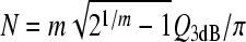 (e.g., Hartmann 1997), which reduces to the value for the mass on a spring (harmonic oscillator) when m = 1. More generally, for filters of arbitrary type, suppose we denote the filter center frequency by CF and bandwidth by Δfx, where Δfx can be any convenient measure of bandwidth, such as BW3dB, BW10dB, or the equivalent rectangular bandwidth (ERB). Then, if the filter phase changes by an amount Δϕx over the interval Δfx, the peak phase-gradient delay will be approximately N ≅ −(Δϕx/Δfx)CF, in periods of the center frequency. By introducing the corresponding Q value, Qx ≡ CF/Δfx, one can write the delay in the form
 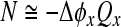 . Thus, because the phase change Δϕx is largely independent of bandwidth in filters of fixed order, the sharpness of tuning (Qx) and filter delay (N) vary together in roughly constant proportion. The top side of the triangle in Figure 1 represents the hypothesis that an analogous relationship between tuning bandwidth and delay applies within the mammalian cochlea.
Evaluation in the chinchilla
We evaluate the relationship between cochlear tuning and delay in chinchilla using Wiener-kernel measurements from the auditory nerve (Recio-Spinoso et al. 2005; Temchin et al. 2005). Figure 4 demonstrates the covariation of chinchilla cochlear tuning and group delay expected from filter theory. The upper panel shows values of QERB (defined as CF/ERB) and NBM (the near-CF phase-gradient delay in periods of the characteristic frequency) obtained from the chinchilla Wiener kernels. Reflecting the systematic variation in cochlear tuning evident in Figure 2A, the values of QERB start off small (near 1–2) at the apical, low-frequency end of the cochlea and increase uniformly with CF, reaching 10–20 at the basal end. As expected from filter theory, the corresponding values of near-CF cochlear delay track this longitudinal variation in the sharpness of tuning. Paralleling the increase in QERB, the delay NBM rises from about 1 cycle of the characteristic frequency in the apex (∼10 ms at 100 Hz) to almost 10 cycles in the base (∼0.5 ms at 20 kHz). Although individual Wiener kernels display some variability, the lower panel shows that the ratio QERB/NBM stays nearly constant along the cochlea. Linear regression suggests a statistically borderline trend for the ratio to increase slightly at higher CFs; on a log(CF) axis, the best-fit slope and its 95% confidence interval are 0.034 ± 0.038. Averaged across CF, the ratio QERB/NBM has the value 1.25 ± 0.02, where the uncertainty represents the standard error of the mean. All told, the estimate 1.25NBM explains 90% of the variance in the measured values of QERB. Interpreted using filter theory, approximate constancy of the ratio QERB/NBM suggests that although the shape of the cochlear filters may vary with CF, their order stays nearly the same.
FIG. 4.

Covariation of cochlear tuning and delay in the chinchilla. The top panel shows values of QERB (circles) and NBM (gray squares) computed from 113 Wiener-kernel measurements of the amplitude and phase of cochlear tuning obtained from auditory-nerve responses to near-threshold noise (Recio-Spinoso et al. 2005). The bottom panel shows the ratio QERB/NBM (triangles) computed from individual Wiener kernels. Values of QERB were obtained from the Wiener-kernel magnitude using standard algorithms (e.g., Evans and Wilson 1973); values of NBM were computed from the gradient of the Wiener-kernel phase near CF. Loess trend lines (Cleveland 1993) have been drawn to guide the eye.
Relation between cochlear delay and otoacoustic delay
Prediction from coherent-reflection theory
Coherent-reflection theory relates the properties of otoacoustic emissions to the mechanical responses of the cochlear partition (Zweig and Shera 1995; Talmadge et al. 1998; Shera et al. 2005). Figure 5 shows a cochlear model in which the uncoiled scalae appear as a fluid-filled box subdivided by a flexible membrane representing the cochlear partition. Standard models assume that the mechanical properties of the partition vary smoothly and monotonically with position. To render the model biologically more realistic, we assume that the impedance of the partition manifests micromechanical irregularities arising from the discrete cellular architecture of the organ of Corti (cf. Engström et al. 1966; Bredberg 1968; Wright 1984; Lonsbury-Martin et al. 1988). These intrinsic irregularities appear superposed on the smooth base-to-apex variation of mechanical characteristics responsible for the tonotopic map. Although micromechanical irregularities may seem a trifling addition, their immediate dynamical consequence is the emission of sound from the model ear. Analysis of the equations shows that irregularities in any mechanical parameter (e.g., the effective damping of the partition) give rise to reverse-traveling waves that return to the ear canal as sound. The model explains the generation of stimulus-frequency and transient-evoked OAEs as the consequence of the coherent “backscattering” of forward-traveling waves (Shera and Zweig 1993).
FIG. 5.

Cross-sectional slice through the symmetric two-dimensional box model. A pure-tone stimulus pressure presented in the ear canal (Pstim) vibrates the stapes and creates a traveling wave visible in the motion of the basilar membrane. Irregularities in the mechanics of the partition (bottom panel) give rise to reverse-traveling waves that return to the ear canal as sound (PSFOAE). Adapted from figure 1 of Shera et al. (2008).
By solving the model equations using perturbation theory (Shera et al. 2005), one can show that the SFOAE pressure, PSFOAE(f), takes the form
 |
1 |
where Pstim is the ear-canal stimulus pressure, GME(f) characterizes round-trip middle-ear transmission, and F is a known functional1 that captures the effects of wave scattering within the model cochlea. The arguments of F describe the distribution of mechanical irregularities and the form of the model traveling wave. The three arguments are: (1) the dimensionless function ε(x,f), which characterizes the type and spatial pattern of the model’s intrinsic irregularities; (2) the model BM velocity normalized by the stapes velocity, VBM(x,f); and (3) the complex wavenumber of the traveling wave, k(x,f), multiplied by the height, H, of the model scalae.
Equation (1) can be used to find the SFOAEs predicted by a given cochlear model. After specifying the necessary parameters and using the model to determine the traveling waves and wavenumbers, one need only evaluate the functional in Eq. (1) to compute the SFOAEs produced by the model. In general, one finds that the predicted SFOAE phase-gradient delays are proportional to the near-CF group delays of the model BM transfer functions (e.g., Shera et al. 2005).2 The left side of the triangle in Figure 1 represents the hypothesis that this proportionality between cochlear and otoacoustic delays applies not only to the broad class of cochlear models from which Eq. (1) was derived but also to the mammalian cochlea.
Evaluation in the chinchilla
We evaluate the relationship between cochlear and otoacoustic delays in chinchilla by (1) using neural estimates of BM motion to derive model predictions for chinchilla SFOAEs and (2) comparing the predicted SFOAEs and their delays with otoacoustic measurements. To obtain model predictions for chinchilla SFOAEs, one must evaluate Eq. (1) for PSFOAE using parameters appropriate for the species. The two most critical quantities to determine are the traveling wave, VBM(x,f), and its wavenumber, k(x,f). Both of these can be found (Shera 2007) using the Wiener-kernel estimates of cochlear tuning (Recio-Spinoso et al. 2005). Estimates of the scalae height are available from anatomical measurements (Salt 2001). Spatial irregularities presumably occur in most, if not all, mechanical parameters; we assume that the dominant contribution arises from the active forces responsible for traveling-wave amplification. Finally, because we are interested in predicting SFOAE phase gradients rather than absolute emission levels, the factor GME describing middle-ear transmission can safely be ignored. Although the phase of GME introduces a delay, middle-ear delay appears negligible compared to traveling-wave delay in chinchilla (Ruggero et al. 1990; Songer and Rosowski 2007). Complete descriptions of the procedures and assumptions involved in deriving model predictions for chinchilla are provided elsewhere (Shera et al. 2008).
Figure 6 compares chinchilla SFOAE magnitude and phase (panel A) with example SFOAEs simulated using the coherent-reflection model (panel B). The simulations were computed from Eq. (1) with parameters adapted to chinchilla using a measured ANF Wiener-kernel estimate of VBM(x,f) and the wavenumber derived from it (CF ≅ 9 kHz). Each of the 17 simulations uses the same Wiener kernel (simulations performed using other Wiener kernels with nearby CFs give similar results) but employs a different random pattern of irregularities; each of the 17 measurements represents a different chinchilla (Siegel et al. 2005). The figure demonstrates that the model reproduces the major features of the measured SFOAEs, including their notchy magnitude functions, correlated undulations in magnitude and phase, and steep mean phase gradients. In both cases, mean phase-gradient delays are approximately 1.4 ms.
FIG. 6.

Measured and simulated chinchilla SFOAEs. Panel (A) shows SFOAE magnitudes and phases measured in 17 chinchillas at 30 dB SPL (Siegel et al. 2005). Panel (B) shows simulated SFOAEs computed from Eq. (1) for PSFOAE(f) with parameters derived from a measured ANF Wiener-kernel estimate of VBM(x,f) (Recio-Spinoso et al. 2005). Each of the 17 model curves was computed using a different irregularity function (sample of Gaussian spatial noise). Both measured and simulated SFOAEs are shown in a frequency range near the Wiener-kernel CF (≅9 kHz). In panel (A), the measurement noise floor lies at about −25 dB SPL, a few decibels below the deepest notches (see figure 4 of Siegel et al. 2005). We cannot confidently predict absolute emission levels (in dB SPL) from the model because we do not know the size of the irregularities and the ANF Wiener kernels provide only a relative measure of tuning. Adapted from figure 4 of Shera et al. (2008).
Both the measurements and the model show considerable variability from animal to animal (or simulation to simulation). Because the model predictions shown in Figure 6 are based on parameters derived from a single Wiener kernel, and take no account of variable factors such as middle-ear transmission, they do not capture the full range of emission levels apparent across animals. The model does, however, capture most of the intrinsic variation apparent in the phase, and thus in the phase-gradient delay. For the simulations shown in Figure 6, the variations in emission magnitude and phase, both from curve to curve at fixed frequency and across frequency in a single simulation, arise entirely from the pattern of irregularities. As explained by coherent-reflection theory, SFOAE generation is analogous to passing noise through a bandpass filter (Zweig and Shera 1995). In this analogy, the “noise” is spatial (i.e., the irregular spatial arrangement and strength of the impedance perturbations that scatter the wave) and the “bandpass spatial filter” results from traveling-wave-induced interference among the multiple wavelets originating within the scattering region.
Figure 7 illustrates the relationship between otoacoustic and cochlear delays predicted by the model and tests the prediction of approximate proportionality using chinchilla data obtained at CFs throughout the cochlea. Figure 7A shows model delay ratios—defined as mean SFOAE phase-gradient delay divided by near-CF BM delay at the same frequency—computed from Eq. (1) with parameters tailored to chinchilla. Individual squares represent model predictions computed using parameters separately derived from 87 different Wiener kernels with CFs spanning almost the full range of chinchilla hearing. Although the predicted delay ratios show considerable scatter due to measurement noise and, perhaps, to intrinsic differences in the characteristics of tuning, the trend line is nearly constant, reflecting the approximate proportionality between mean otoacoustic and cochlear delays predicted by the model.
FIG. 7.

Empirical and predicted delay ratios in chinchilla. In panel (A), the filled squares give the ratio of SFOAE delay to near-CF BM delay computed from Eq. (1) for PSFOAE using parameters derived from chinchilla ANF Wiener kernels. In panel (B), the open symbols give empirical delay ratios computed using measured values of SFOAE delay (Siegel et al. 2005). Triangles and circles show results for the total SFOAE and its unmixed (long-latency) component, respectively. In both panels, the corresponding near-CF BM delays (denominator) were obtained from the Wiener-kernel data (Recio-Spinoso et al. 2005; Temchin et al. 2005). Loess trend lines are shown to guide the eye; the model trend from panel (A) is reproduced in panel (B). Adapted from figure 10 of Shera et al. (2008).
Does the proportionality between otoacoustic and cochlear delays predicted by the model apply to the actual chinchilla data? The triangles in Figure 7B show delay ratios computed by combining the measured SFOAE delays (numerator) with the Wiener-kernel estimates of near-CF BM delay (denominator). At frequencies above about 4 kHz, the trend is flat and agrees closely with the model predictions. Indeed, the two distributions (empirical triangles and predicted squares) are statistically indistinguishable in this region (Kolmogorov–Smirnov or KS test). Below 4 kHz, however, the empirical delay ratios decrease below model predictions, even, somewhat paradoxically, falling substantially below one (Siegel et al. 2005).
Extrapolating from the model’s success in the high-frequency base, and noting what appear to be interference notches sometimes observed in low-frequency chinchilla SFOAEs, we suggest elsewhere (Shera et al. 2008) that the paradoxically small delay ratios result from the existence of an additional SFOAE generation mechanism that produces an emission component with a shallow phase slope (i.e., short phase-gradient delay). We hypothesize that this additional mechanism, not accounted for in the model, may exist throughout the cochlea but becomes more powerful at low frequencies. Unmixing the measured SFOAEs using signal-processing algorithms that separate components based on latency yields short- and long-latency components with phase gradients and amplitude characteristics consistent with this hypothesis (Shera et al. 2008). For example, the circles in Figure 7B show empirical delay ratios computed using only the long-latency component extracted from the total SFOAE. Removing the short-latency component has a negligible effect above 4 kHz but extends the predicted proportionality between the (long-latency) SFOAE delay and near-CF BM delay throughout the cochlea. Empirical delay ratios computed using the long-latency component (circles) are statistically indistinguishable from predictions (squares) in both the apex and the base (KS test). Thus, the long-latency component (real in the base, putative in the apex) appears everywhere consistent with an origin via coherent reflection. In “Criticisms, clarifications, and unresolved issues”, we speculate about possible mechanisms responsible for the short-latency emission apparent at low frequencies (see also Shera et al. 2008). As discussed further in subsequent sections, otoacoustic evidence such as that presented in Figure 7B argues for a transition between “apical-like” and “basal-like” behavior in mammalian cochlear mechanics.
Relation between cochlear tuning and otoacoustic delay
Prediction from the triangle
Covariation of cochlear tuning and otoacoustic delay is predicted by their mutual relationship to cochlear delay, the third vertex of the triangle. The logic of the prediction is transitive: If A ∼ B and B ∼ C then A ∼ C. Measurements in both cats and guinea pigs reveal a strong empirical covariation across frequency between QERB values, as obtained from auditory-nerve fibers, and SFOAE phase-gradient delay (NSFOAE) in stimulus periods (Shera et al. 2002; Shera and Guinan 2003).
Evaluation in the chinchilla
Figure 8 extends these empirical relationships to chinchillas, demonstrating that QERB and NSFOAE vary together with frequency, as predicted by the logic of the triangle. In all three species, the sharpness of tuning and SFOAE delay change roughly in parallel, increasing from minimum values at frequencies mapping to the apex of the cochlea to maxima at frequencies in the base. The covariation of ANF tuning and SFOAE delay is not unique to mammals; a similar relationship has been established, and accounted for using models of OAE generation, in the tokay gecko and alligator lizard (Bergevin and Shera 2010).
FIG. 8.

Empirical covariation of cochlear tuning and otoacoustic delay in three species. The three columns of the top row show values of QERB computed from auditory-nerve fibers in cat, guinea pig, and chinchilla, respectively (left to right). The bottom row shows corresponding values of NSFOAE, the SFOAE phase-gradient delay in stimulus periods. Loess trend lines (Cleveland 1993) are shown to guide the eye. The auditory-nerve data in cat come from studies by Delgutte and colleagues (e.g., Cedolin and Delgutte 2005), the data in guinea pig from Tsuji and Liberman (1997), and the data in chinchilla from Recio-Spinoso et al. (2005). The otoacoustic data in cat and guinea pig come from Shera and Guinan (2003) and in chinchilla from Siegel et al. (2005).
Applications: otoacoustic estimation of cochlear tuning
Having established that physiological data from chinchilla generally support the triangle of hypothesized relationships, we now apply the framework to estimate cochlear tuning noninvasively. The quantitative procedure outlined below, an extension and refinement of that proposed earlier (Shera et al. 2002), builds upon the empirical relationship between QERB and NSFOAE illustrated in Figure 8.
Tuning ratios and their unification
The covariation of cochlear tuning and otoacoustic delay demonstrated in Figure 8 implies that the ratio of the two varies substantially less than either individually. To quantify the empirical relationship between them, we define the “tuning ratio” rspecies(CF) for a given species as the frequency-dependent quotient3
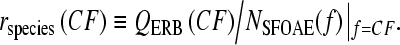 |
2 |
We emphasize that tuning ratios are defined using the otoacoustic delay, not the “BM delay”, NBM, used in Figure 4B; NSFOAE is computed from the phase of the total SFOAE—no “unmixing” analysis is performed (cf. Fig. 7). Note that we evaluate the ratio using SFOAE data obtained at frequencies matched to the neural CF. Matching the emission frequency to CF is suggested by coherent-reflection theory, which indicates that SFOAEs originate predominantly from the peak region of the traveling wave, at least in the basal part of the cochlea (see “Relation between cochlear delay and otoacoustic delay”).
Figure 9A shows the tuning ratios for cat, guinea pig, and chinchilla computed from the data in Figure 8. Each species is represented by a single curve; because the values of QERB and NSFOAE for each species were measured in different studies using separate groups of animals, the tuning ratios were computed using the trend lines in Figure 8 rather than individual data points. The three tuning ratios are shown on a spatial axis (fractional distance from the apex) obtained by converting CF to normalized cochlear location using the tonotopic map appropriate to the species (Liberman 1982; Greenwood 1990; Tsuji and Liberman 1997). This normalized spatial coordinate, whose widespread use derives from the suggestion that many mammalian cochleae constitute “scaled” versions of one another (Greenwood 1961; Greenwood 1990), provides a convenient way of comparing species with different frequency ranges of hearing. Although the tuning ratios appear somewhat offset from one another along the horizontal axis, the curves in all three species share a qualitatively similar form. In the basal region, the tuning ratios are nearly constant, varying only slowly with location; in the apical region, they change more rapidly (and also appear somewhat more variable across species).
FIG. 9.

Tuning ratios in cat, guinea pig, and chinchilla. Panel (A) shows the curves rspecies ≡ QERB/NSFOAE computed from the trend lines in Figure 8. The curves are plotted versus cochlear location (fractional distance from the apex), computed using the corresponding cochlear map (Liberman 1982; Greenwood 1990; Tsuji and Liberman 1997). Panel (B) shows the approximate unification achieved when the curves are plotted versus CF/CFa|b, the CF normalized by the apical–basal transition CF. Values of CFa|b for each species are given in Table 1.
An apical–basal transition
The finding that the tuning ratios in the three species appear to be horizontally shifted versions of a curve with the same general shape suggests that normalizing away the location of the transition between the “apical-like” and “basal-like” behavior might collapse them onto a single curve. Indeed, when plotted against the special, normalized frequency axis used in Figure 9B, all three curves nearly overlie one another, indicating that the tuning ratios in these species are quantitatively similar. Approximate unification of the tuning ratios is achieved by regarding r as a function of the normalized characteristic frequency CF/CFa|b,4 where CFa|b is a species-dependent parameter that we call the “apical–basal transition CF.” Table 1 lists approximate values of CFa|b that align the tuning ratios.5 In effect, CFa|b divides the cochlea of a given species into two parts: a high-frequency region of apparently “basal-like” behavior (CF > CFa|b) and a low-frequency region of more “apical-like” behavior (CF < CFa|b). The unification evident in Figure 9B means that in any given species the tuning ratio is well approximated by the formula
 |
3 |
where r is a “universal” or species-invariant curve and CFa|b characterizes the apical–basal transition in the given species.
TABLE 1.
Approximate apical–basal transition CFs in four mammalian species
| CFa|b (kHz) | CFmax/CFa|b | Apical fraction | |
|---|---|---|---|
| Cat | 3 | 19 | 0.4 |
| Guinea pig | 3 | 18 | 0.5 |
| Chinchilla | 4 | 5 | 0.7 |
| Human | 1 | 20 | 0.4 |
The values of CFa|b needed to align the tuning ratios can be estimated from the tuning ratios themselves (for cat, guinea pig, and chinchilla) and/or from plots of NSFOAE (all species; Figs. 8 and 11). Because the estimates, especially those obtained from NSFOAE, are uncertain (by perhaps an eighth to a quarter octave) and because none of our results depend on precise values of CFa|b, we have rounded the values to the nearest multiple of 1 kHz. In each species, approximate values of CFmax/CFa|b and the apical fraction (defined as the proportion of the cochlear length devoted to CFs less than CFa|b) were computed using parameters of the cochlear map (Liberman 1982; Greenwood 1990; Tsuji and Liberman 1997).
Inspection of Figure 8 indicates that the “bend” in the tuning ratios that occurs at frequencies near CFa|b originates primarily in the frequency dependence of NSFOAE, which in all three species manifests a mid-frequency deviation from its high-frequency slope that subsequently shows up in the ratio QERB/NSFOAE (cf. Shera and Guinan 2003).6 The value of CFa|b can therefore be estimated from plots of NSFOAE(f ) alone, without reference to the neural measurements. In chinchilla, the deviation from the high-frequency behavior appears in Figure 7B as a decrease in the total SFOAE delay (re BM delay) at frequencies below about 4 kHz (i.e., below the approximate value of CFa|b). At these lower frequencies, the mechanism responsible for the short-latency emission component (cf. “Relation between cochlear delay and otoacoustic delay”) contributes significantly to the total SFOAE. As discussed in “Significance of the apical–basal transition”, the value of CFa|b determined from the tuning ratios and OAE measurements matches the CF associated with other significant apical–basal changes in cochlear mechanics and physiology (cf. Shera and Guinan 2003; Shera 2007; Temchin et al. 2008).
Validation of otoacoustic estimates of tuning in the chinchilla
To find the sharpness of tuning from otoacoustic measurements we exploit the approximate species-invariance of the tuning ratio. In particular, we estimate tuning from measurements of NSFOAE by solving Eq. (2) for QERB:
 |
4 |
Figure 10 illustrates the procedure in chinchilla. The figure shows otoacoustic estimates of chinchilla QERB computed from Eq. (4) using the trend of the chinchilla NSFOAE measurements from the bottom panel of Figure 8C (Siegel et al. 2005). Two OAE-based estimates of QERB are shown, one obtained using the cat tuning ratio (rcat) and the other obtained using the guinea pig ratio (rguinea pig). Comparison with QERB values obtained directly from the chinchilla auditory nerve (Recio-Spinoso et al. 2005) demonstrates the validity of the otoacoustic values. Whether taken separately or together, the two otoacoustic estimates derived from NSFOAE and tuning ratios in cat and guinea pig account for about 75% of the variability in the neural measurements.
FIG. 10.

Otoacoustic estimates of chinchilla cochlear tuning. The dashed lines give values of chinchilla QERB computed from Eq. (4) using measured SFOAE delays (from figure 8c of Siegel et al. 2005) and tuning ratios for cat and guinea pig (Fig. 9B). The open circles and solid trend line give measured values derived from the ANF Wiener kernels (Recio-Spinoso et al. 2005).
Because of the order in which we have presented the material, the close agreement between the otoacoustic estimates and the neural measurements of QERB evident in Figure 10 was entirely predictable from earlier figures. Since we have already established that the tuning ratios used in the calculations (rcat and rguinea pig) are essentially indistinguishable from the tuning ratio in chinchilla (cf. Fig. 9B), the procedure was guaranteed, in retrospect, to yield reasonable estimates of chinchilla tuning. Figure 10 is therefore an alternate, albeit perhaps more suggestive way of presenting the near-equivalence of the tuning ratios in these three species. The figure demonstrates, however, that if neural measurements of chinchilla tuning had been unavailable, and we had had to rely entirely on the otoacoustic estimates derived from Eq. (4), we would have obtained physiologically accurate estimates of QERB.
Application to humans
We estimate the sharpness of human cochlear tuning from otoacoustic measurements by assuming that the species-invariance of the tuning ratio demonstrated here in cat, guinea pig, and chinchilla extends also to human (Shera et al. 2002). Computing human values of QERB (CF) requires knowledge of human SFOAE delays and an estimate of the human apical–basal transition CF. Figure 11 shows measurements of NSFOAE in both humans (Dreisbach et al. 1998; Shera and Guinan 2003) and chinchilla (Siegel et al. 2005). Comparison of the trend lines in the two species shows that at any given frequency human SFOAE delays are never less than three and often as much as ten times longer than their counterparts in chinchilla. Interpreted according to the triangle of relationships, longer OAE delays suggest sharper cochlear tuning.
FIG. 11.

SFOAE group delays in humans and chinchillas. Filled triangles give values of NSFOAE (SFOAE group delay in periods of the stimulus frequency) vs frequency. Upward triangles are from Shera and Guinan (2003); downward triangles with error bars are from Dreisbach et al. (1998). Gray circles show NSFOAE in chinchilla (Siegel et al. 2005). Loess trend lines for both species are shown to guide the eye. Sloping dashed lines show power-law fits to the high-frequency data. Vertical dashed lines mark the approximate location where the trend line departs from the power-law fit, providing an estimate of CFa|b.
We indicate our rough estimates of CFa|b in Figure 11 using vertical dashed lines. As discussed above, one can approximate CFa|b in each species as the location of the deviation from the high-frequency power-law behavior in NSFOAE(f). For example, the sloping dashed lines in Figure 11 show a power-law fit (i.e., a straight line on these log–log axes) to the high-frequency data. For each species, the dashed vertical line at CFa|b then identifies the approximate frequency where the solid trend line deviates from its high-frequency, power-law form. Although the human data in Figure 11 are sparse at low frequencies, data from other OAE studies provide corroborating evidence for a transition between apical-like and basal-like behavior in the 1–2 kHz region of the human cochlea (e.g., Schairer et al. 2006; Bergevin et al. 2008). The estimate CFa|b ≅ 1 kHz implies that the apical–basal transition in humans—like that in cats and guinea pigs, but unlike that in chinchillas—occurs near the mid-point of the cochlea, at a CF roughly four octaves below the maximum frequency of hearing (cf. Table 1).
Estimates of the sharpness of human tuning can now be obtained by evaluating Eq. (4) using the tuning ratios r(CF/CFa|b) from Figure 9B, the values of CFa|b from Table 1, and the human trend for NSFOAE(f) from Figure 11. Figure 12 shows the resulting functions QERB(CF). The estimates of human tuning obtained using the tuning ratios from cat, guinea pig, and chinchilla are shown using different shades of gray. The three estimates of QERB(CF) almost overlap because the tuning ratios r(CF/CFa|b) in the three species are nearly identical. Although the otoacoustic estimates of QERB(CF) are similar to those derived previously (Shera et al. 2002), our revised procedures have extended the estimates to CFs below 1 kHz.
FIG. 12.

Otoacoustic estimates of human cochlear tuning. The solid lines give values of human QERB computed from Eq. (4) using measured values of NSFOAE (Fig. 11) and tuning ratios for cat, guinea pig, and chinchilla (Fig. 9B). Black circles and squares give behavioral estimates reproduced from figure 5 of Oxenham and Shera (2003); error bars show the associated standard error of the mean. For comparison, the dashed lines give QERB values for cat, guinea pig, and chinchilla obtained from ANF measurements. Abbreviations (ct, gp, ch) identify values derived from measurements in each of the three species (cat, guinea pig, chinchilla).
For comparison with the human estimates, Figure 12 reproduces the values of QERB(CF) obtained from auditory-nerve recordings in the three laboratory species (top panels of Fig. 8). Also shown are human behavioral values obtained using psychophysical methods designed both to minimize the effects of suppression and compression and to mimic the measurement of neural tuning curves (Oxenham and Shera 2003). Although the otoacoustic and behavioral estimates of QERB(CF) derive from qualitatively different types of measurements, they nevertheless appear in remarkable quantitative agreement. Both indicate that human cochlear tuning is perhaps two to three times sharper than that measured in laboratory animals but depends similarly on CF. The overall power-law trend toward sharper tuning at higher CFs matches the animal measurements but disagrees with the standard view of almost constant QERB in the base (e.g., Glasberg and Moore 1990).
The difference between the human otoacoustic values of QERB and the measurements in the other species is not just an artifact of our estimate of the human apical–basal transition CF. Indeed, using alternate values for CFa|b in humans only exacerbates the apparent differences between the species. For example, Figure 13 shows the otoacoustic values of QERB derived by assuming that the human value of CFa|b equals the value in chinchilla (4 kHz). Not only are the estimates of human tuning derived using this chinchilla-based choice of CFa|b sharper than those obtained using the 1-kHz transition frequency, but the resulting function QERB(CF) manifests a non-monotonic dependence on CF unlike anything seen in the neural measurements.
FIG. 13.

Otoacoustic estimates of human QERB obtained using CFa|b appropriate for chinchilla. The dashed lines show values of QERB computed from Eq. (4) using the apical–basal transition CF for chinchilla (CFa|b ≅ 4 kHz). The solid lines, reproduced from Figure 12, show QERB values computed using the human estimate (CFa|b ≅ 1 kHz).
Discussion
This paper combines diverse experimental data to test the hypothesis that cochlear tuning, cochlear delay, and otoacoustic emissions are mutually interrelated via a theoretical framework whose broad outlines are represented by the triangle in Figure 1. Although the triangle is an imperfect distillation of complex relationships, it provides a useful conceptual foundation for organizing and understanding multiple aspects of cochlear function. With one important exception, auditory-nerve and OAE measurements in chinchilla (Recio-Spinoso et al. 2005; Siegel et al. 2005; Temchin et al. 2005) corroborate all hypothesized relationships, including predictions from filter theory and the coherent-reflection model of OAE generation. The exception involves low-frequency SFOAEs, whose phase-gradient delays are anomalously short relative to mechanical or neural delays in all mammalian species so far examined (Shera and Guinan 2003; Siegel et al. 2005). The apparent dissociation between cochlear and OAE delay in the apex appears as a blessing in disguise; it both implies the existence of regions of “apical-like” and “basal-like” behavior in the cochlea and allows noninvasive estimation of the species-dependent parameter, CFa|b, that locates the approximate boundary between the two.
The hypotheses validated here support the use of reflection-source OAE phase-gradient delays as noninvasive probes of cochlear tuning (e.g., Shera et al. 2002; Schairer et al. 2006; Sisto and Moleti 2007). Both our original procedure (Shera et al. 2002) and its current refinement exploit empirical relationships between QERB and NSFOAE (i.e., the right side of the triangle in Fig. 1) to infer information about cochlear tuning from SFOAE measurements. Although the other two sides of the triangle (i.e., those involving filter theory and/or the mechanisms of OAE generation) play no direct role in the analysis, they serve to emphasize that the correlations underlying the procedure have multiple sources of empirical and theoretical support. Considered in isolation, the relation between QERB and NSFOAE (Fig. 8) represents a useful but seemingly fortuitous empirical correlation; the other sides of the triangle buttress the argument by providing a framework for understanding how and why the observed relationships come about. Indeed, the existence of the relationships shown in Figure 8 was first deduced on theoretical grounds by combining ideas from filter theory and coherent reflection to predict the existence of an empirical covariation between QERB and NSFOAE.
By exploring the empirical relationships between QERB and NSFOAE, we have shown that tuning ratios (QERB/NSFOAE) regarded as a function of CF/CFa|b have a nearly species-invariant form in cat, guinea pig, and chinchilla. We suggest that normalizing by CFa|b provides a transformation of the CF axis that helps to compensate for mechanical and physiological differences between the base and apex of the cochlea. Were it to hold more generally, approximate species-invariance of the tuning ratio would imply that estimates of cochlear tuning could be derived from SFOAE delays. By quantifying this idea, we demonstrate that otoacoustic estimates of chinchilla cochlear tuning match direct physiological measures obtained from the auditory nerve (Recio-Spinoso et al. 2005).
The procedure developed here differs in three principal respects from that employed previously (Shera et al. 2002). First, the current procedure evaluates QERB using the tuning ratios themselves (i.e., the curves in Fig. 9B) and the trend lines for NSFOAE(f ) in Figure 8 rather than power-law fits to these quantities. Second, the procedure employs data from both the apical and basal parts of the cochlea, rather than from just from the basal part. Third, the procedure uses Eq. (4) and therefore evaluates the tuning ratios for different species at corresponding values of CF/CFa|b, rather than at corresponding cochlear locations. With regard to this last point, the chinchilla data make clear what was previously uncertain—namely, that tuning ratios (and/or the locations of the bends in NSFOAE curves) are not especially invariant across species if evaluated at constant cochlear location. As a result, the previous estimation procedure7 appears unreliable, at least in chinchilla.
Extending (by assumption) the approximate species-invariance of the tuning ratio to humans yields otoacoustic estimates of cochlear tuning that agree well with previous estimates (Shera et al. 2002). Our otoacoustic estimates of QERB in human are mutually consistent with independent behavioral measurements obtained using completely different rationales, methodologies, and analysis procedures (Oxenham and Shera 2003). To put it another way, the evident agreement between the otoacoustic and behavioral estimates of tuning implies that human tuning ratios rhuman = QERB/NSFOAE computed from the behavioral values of QERB and the otoacoustic measurements of NSFOAE closely match the tuning ratios found in cat, guinea pig, and chinchilla.
Criticisms, clarifications, and unresolved issues
In addition to challenging the framework tested here in chinchilla, other investigators have raised specific criticisms regarding its application to the estimation of human cochlear tuning (e.g., Ruggero and Temchin 2005; Siegel et al. 2005; Ruggero and Temchin 2007). Although many of the criticisms dissipate upon clearer understanding of the procedures, many also touch upon important issues that warrant further discussion. In the following, we list the major criticisms of our previous work (Shera et al. 2002; Oxenham and Shera 2003)—and, by extension, of the revision presented here—together with our clarifications and remarks.
-
The procedure for estimating tuning relies on an incorrect model of OAE generation. Although we motivate the analysis using insight derived from theoretical models, the procedure we employ is fundamentally empirical and does not rely on any model of OAE generation. The key assumption is that the relation between cochlear tuning and OAE delay established in laboratory animals applies also to humans. Thus, even major revisions to current understanding of OAE generation would leave the outcome of the procedure unchanged.
Regarding the coherent-reflection model, we have shown both that the model works well in the base of the cochlea and that the situation is more complex in the apex (Shera et al. 2008). As demonstrated in Figure 7, when parameters are derived using chinchilla auditory-nerve data, the model correctly predicts chinchilla SFOAE delays at frequencies greater than 3–4 kHz (i.e., above CFa|b). At lower frequencies, we have presented evidence for multiple emission components that complicate the interpretation (Shera et al. 2008). At low frequencies, chinchilla SFOAE spectra sometimes manifest what appear to be regularly spaced interference notches, suggesting that low-frequency SFOAEs consist of two principal components with similar amplitudes but different phase-gradient delays. Separating these putative components using signal-processing techniques yields short- and long-latency components with phase gradients and amplitude characteristics consistent with this suggestion. In particular, the phase-gradient delay of the long-latency component matches the delay predicted by the model (Fig. 7; see also Shera et al. 2008). These results both support the coherent-reflection model, so far as it goes, and indicate that additional, as yet unidentified, mechanisms are operating in the apex of the cochlea to generate the short-latency OAE component.
Although definitive conclusions about the putative long-latency component of low-frequency SFOAEs predicted by coherent-reflection theory require independent corroboration of the unmixing analysis, there can be no doubt about the existence of the significant short-latency SFOAE at low frequencies. In all mammalian species so far examined, and even a few lizards (Bergevin and Shera 2010), low-frequency SFOAE phase-gradient delays appear anomalously short when compared either to near-CF mechanical and neural delays or to extrapolations based on OAE delays measured at higher frequencies (Shera and Guinan 2003; Siegel et al. 2005). Indeed, it is precisely the departure from the high-frequency trend that produces the “bend” in NSFOAE(f) and provides a rough estimate of the apical–basal transition frequency, CFa|b.
Potential sources of the short-latency SFOAE are suggested elsewhere (Shera and Guinan 2003; Shera et al. 2008). They include contributions from (1) measurement artifacts, such as noise or a breakdown in the assumptions about cochlear nonlinearity and the effect of the suppressor tone that underlie the measurement of SFOAEs (e.g., Kalluri and Shera 2007a); (2) nonlinear reflection by wave-induced perturbations in the mechanics (e.g., Talmadge et al. 2000); (3) emission components arising from the “tail” region of the traveling wave (e.g., Siegel et al. 2003; Siegel et al. 2004; Choi et al. 2008); and/or (4) additional modes of motion or energy transport beyond those associated with the classical traveling wave (e.g., Guinan et al. 2005; Ghaffari et al. 2007; Karavitaki and Mountain 2007; Guinan and Cooper 2008). The extensive list of possibilities, none mutually exclusive, highlights how much about apical cochlear mechanics, including mechanisms of emission generation, remains unknown.
-
The procedure for estimating tuning relies on an incorrect relationship between SFOAE delays and near-CF BM delays. In fact, the procedure does not rely on any relationship between SFOAE and BM delays. The procedure is based on tuning ratios, which are constructed from measurements of QERB and NSFOAE; BM delays do not appear in the calculations.
In our previous publication (Shera et al. 2002), however, we were too clever by half: We motivated the discussion by dividing NSFOAE by two in order to compensate for round-trip travel and thereby obtain an estimate of near-CF “BM delay.” This was a mistake, for two reasons. First, it gave the erroneous impression that the tuning estimates actually depended on the factor of two. As the formulae in that paper make clear, however, this is not the case. Indeed, we could have divided NSFOAE by any number whatsoever, so long as the number was the same across species, and the tuning estimates would have been unchanged. Second, dividing SFOAE delays by two, although intuitively appealing, does not yield especially good estimates of BM delay (cf. Fig. 7; see also Shera and Guinan 2003; Siegel et al. 2005). Improved theoretical analysis, motivated by discrepancies between model predictions and experiment (Shera and Guinan 2003; Siegel et al. 2005), has since shown that dividing the OAE delay by two provides better estimates of the near-CF delay of the pressure-difference wave (Shera et al. 2008). Although closely related, the delays associated with BM traveling waves and with pressure-difference waves are not identical. Thus, rather than trying to motivate the procedure by dividing NSFOAE by a number whose value was both empirically uncertain and logically irrelevant, we should have left estimates of BM delay entirely out of the analysis, as we do in this paper.
-
Human BM delays are similar to those measured in laboratory animals. Although BM delays are not directly relevant to our procedure (which infers QERB from NSFOAE; see item #2 above), determining their magnitude in humans remains an outstanding issue with important implications both for cochlear mechanics and for the validity of the human triangle of relationships. Unfortunately, human BM delays cannot be directly measured and must be inferred. Ruggero and Temchin (2007) calculate human delays using the equation
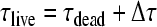 , where the subscripts denote pre- and post-mortem BM delays and Δτ indicates the change due to death. After noting that compiled data suggest similar values of τdead across species (including human cadavers),8 Ruggero and Temchin assume that human values of Δτ are also similar to those measured in laboratory animals.9 This assumption enables them to calculate τlive in humans. Thus, by construction, they find that human BM delays are similar to those measured in laboratory animals.
One might object that our procedure for estimating human tuning also assumes similarity across species (i.e., approximate invariance of the tuning ratio). Have we not therefore merely begged the same question and manufactured another circular argument, albeit one involving tuning rather than delay? The important distinction, we argue, is that our procedure makes no assumption about the quantity of interest. We do not assume, directly or indirectly, that humans have sharper tuning; rather, we deduce values of QERB from measurements of human SFOAE delay interpreted using the triangle of relationships.
In this regard, all studies agree that human SFOAE delays are substantially longer than those in common laboratory animals. Although the qualitative picture is clear, quantitative details that could affect our numerical estimates of QERB remain unsettled. In particular, the literature contains differing estimates of the value and frequency dependence of human SFOAE delay, especially above 2 kHz. Although the NSFOAE data employed here (Dreisbach et al. 1998; Shera and Guinan 2003) are similar to those measured by Bergevin et al. (Bergevin et al. 2008) and appear consistent with delays inferred from spontaneous-emission spacings (Shera 2003), other studies have found somewhat different results. For example, Schairer et al. (2006) report smaller values of NSFOAE and a shallower frequency dependence. Studies using transient emissions, which are expected to have delays similar if not identical to those of SFOAEs (Kalluri and Shera 2007b), also disagree with one another at high frequencies: Whereas Sisto and Moleti (2007) report longer delays and a somewhat stronger dependence on frequency than suggested by the values of NSFOAE used here, Goodman et al. (2009) report the opposite. These quantitative disparities need to be resolved before truly reliable estimates of human cochlear tuning and delay can be obtained from OAE measurements. Whether the disagreements reflect differences in measurement methodology, data analysis, stimulus intensity, subject population, and/or other factors remains unclear. As a control for some of these issues, and because our procedure for estimating QERB from NSFOAE is fundamentally comparative, we took care to employ the same OAE measurement and analysis procedures in humans and laboratory animals whenever possible.
Notwithstanding the various differences among studies, it is an empirical fact that human OAE delays are substantially longer than those of common laboratory animals. Whatever its flaws and remaining uncertainties, the framework schematized by the triangle of relationships explains this observation. Criticisms of the framework based on assertions that human tuning and delays are similar to those in laboratory animals would have more force were they able to provide an alternative plausible answer to this one question: If human cochlear tuning and traveling-wave delays are just like those in laboratory animals, why are human otoacoustic delays so long?
Behavioral measurements based on forward masking overestimate the sharpness of cochlear tuning. This objection (Ruggero and Temchin 2005) stems from animal studies that measured behavioral tuning using tonal forward maskers and found bandwidths that were, for the most part, narrower than those of ANF tuning curves in the same or similar species (e.g., McGee et al. 1976; Kuhn and Saunders 1980; Serafin et al. 1982). It has been well known in the human psychophysical literature since the 1970s that the use of tonal forward maskers can lead to implausibly narrow estimates of tuning (e.g., Moore 1978). In the 30 years since, psychophysicists have made considerable progress identifying the potential artifacts (e.g., off-frequency listening and “confusion” between a masker and signal of the same frequency) and devising methods to minimize them (e.g., Moore and Glasberg 1981; O’Loughlin and Moore 1981; Moore et al. 1984; Neff 1985). The method used by Oxenham and Shera (2003), known as the notched-noise method (Patterson 1976), was designed to circumvent these known confounds. Thus, the criticism of Ruggero and Temchin (2005) applies to animal psychophysical studies of 30 years ago, but not to more recent psychophysical estimates in humans. To date, no studies in other species have used the methods employed by Oxenham and Shera in a behavioral paradigm. Filling this void in the literature would help complete another important triangle of relationships: neural, otoacoustic, and behavioral estimates of tuning in the same species.
Significance of the apical–basal transition
Most of what we know about cochlear mechanics and OAE generation comes from measurements performed in the basal, high-frequency half of the cochlea. There is mounting evidence, however, that the apical half manifests significant differences (e.g., Cooper and Rhode 1997; Shera and Guinan 2003; Guinan et al. 2005; Nowotny and Gummer 2006; Shera 2007; Temchin et al. 2008). Consistent with this view, the unification of the tuning ratios achieved in cat, guinea pig, chinchilla, and human (when the psychophysical data shown in Fig. 12 are used for QERB) suggests the existence of a species-dependent parameter, the apical–basal transition CF (CFa|b), that partitions the cochlea into apical-like and basal-like sections based on the behavior of the ratio QERB/NSFOAE.
Although unifying the tuning ratios by aligning the frequency axes to CFa|b might seem just an empty kind of curve shifting, no law of nature requires that the tuning ratios be similar, let alone almost identical. Nevertheless, a simple normalization of the frequency axis transforms the tuning ratios into an approximately species-invariant curve. To help put the values of CFa|b in context, Table 1 provides related numbers for each species. Column 2 gives approximate values of the ratio CFmax/CFa|b, where CFmax is the maximum frequency of the cochlear map. Note that the ratio CFmax/CFa|b is roughly a factor of four smaller in chinchilla than in cat, guinea pig, and human. Thus, the chinchilla transition CF occurs about two octaves “closer” to the stapes than in the other animals. Column 3 shows the fraction of the cochlea with CFs less than CFa|b, computed using the cochlear map. By this measure, roughly two thirds of the chinchilla cochlea is “apical” in character, compared with an average of somewhat less than one half of the cochlea for the other species. Because the values of CFa|b in cat, guinea pig, and chinchilla are similar, normalization by CFa|b is not essential for achieving approximate unification of the tuning ratios in these three species. Similarly, because the apical fractions (column 3) in cat, guinea pig, and human are similar, a rough unification of the tuning ratios in these species can be achieved by plotting them versus normalized cochlear location (e.g., fractional distance from the apex, as in Fig. 9A). Although these other methods provide approximate unification for various subsets of the four tuning ratios, normalization of the CF axis by CFa|b is the simplest transformation that unifies all four simultaneously.
The “bend” in the tuning ratio that occurs near CFa|b largely reflects the frequency dependence of NSFOAE(f) (Shera and Guinan 2003). At least in the chinchilla, the bend appears to be caused by the apical appearance of a significant SFOAE component with phase-gradient delay much shorter than the forward BM travel time. Although SFOAE and near-CF BM or neural delays vary together in the basal half of the cochlea, the close relationship between the two breaks down in the apical half, where SFOAE phase-gradient delays appear anomalously short in all mammalian species so far examined, including humans (Shera and Guinan 2003; Siegel et al. 2005; Banakis et al. 2008). The approximate CF associated with this otoacoustic apical–basal transition depends on species: in cat, guinea pig, and chinchilla the transition occurs near 3–4 kHz; in humans, it appears closer to 1 kHz. The approximate unification of the tuning ratios brought about by aligning the curves to CFa|b shows that the transition located by CFa|b occurs at the same value of the tuning ratio in all four species considered. The consistency of finding that the bend in the NSFOAE data occurs at the same tuning ratio suggests that the underlying cochlear factors that produce the CFa|b transition are closely related to the factors that produce the tuning ratio. With this view, the cochlea becomes “apical-like,” and the short-latency SFOAE component becomes significant, when the tuning ratio exceeds a certain constant value.
Although identifiable using otoacoustic data, the locations of the apical–basal transition in cat, guinea pig, and chinchilla correspond with the CF regions associated with prominent changes in other aspects of cochlear physiology (Shera and Guinan 2003). In all three species, for example, the otoacoustic transition frequency matches the approximate CF at which ANF tuning curves change from the scaling-invariant, classical tip/tail form characteristic of high-CF fibers to the more complex and often multilobed shapes found in the apex (Liberman 1978; Liberman and Kiang 1978; Temchin et al. 2008). Although relevant behavioral data in humans are sparse, and the interpretation less direct, existing data do suggest a transition between scaling and non-scaling behavior near the 1 kHz region of the cochlea (e.g., Moore et al. 1984; Glasberg and Moore 1990; Oxenham and Dau 2001).
In chinchilla, the value of CFa|b locates not only an abrupt change in the shapes of neural tuning curves (Temchin et al. 2008), but also phase changes in the response to low-frequency tones (Ruggero and Rich 1983) and an apparent change in the characteristics of cochlear wave propagation and amplification (Shera 2007). For example, cochlear traveling-wave propagation and gain functions derived from neural data undergo quantitative changes near 4 kHz. In particular, the maximum value of the traveling-wave gain function is generally smaller, and the spatial extent of the amplification region substantially larger, at CFs below 3–4 kHz than at CFs above [see figures 12–14 of Shera (2007)]. Somewhat surprisingly, these prominent apical–basal changes in chinchilla cochlear mechanics and physiology have no obvious effect on the ratio QERB/NBM.10 As demonstrated in Figure 4, the ratio QERB/NBM remains nearly constant throughout the cochlea, suggesting no significant apical–basal gradient in the underlying “type” of filter.
As the large values of the transition CFs make clear, the apical–basal differences manifest here and in other physiological data are not mere mechanical “end effects” caused by proximity to the helicotrema. Presumably they reflect apical–basal changes in organ of Corti micromechanics or modes of motion (e.g., Nowotny and Gummer 2006). Whatever their origin—or origins, for the transitions apparent in the various species and the different physiological measures may not be causally related—they evidently reflect a CF dependence in cochlear mechanics whose significance for auditory signal processing remains to be understood.
Species trends and individual variability
Because the otoacoustic, neural, and psychophysical data employed here were generally obtained from different groups of animals, our evaluation and subsequent application of the triangle of relationships has, for the most part, been limited to population trends. For example, the relationships between cochlear and OAE delay predicted by coherent-reflection theory were tested by deriving model parameters using neural data obtained in one group of chinchillas and comparing the resulting model predictions with SFOAEs measured in another (Figs. 6 and 7). Similarly, we computed the tuning ratios defined by Eq. (2) using loess curves that summarize otoacoustic and neural trends across many animals (Figs. 8 and 9B). Although necessarily limited, analysis at this “species level” is nevertheless extremely informative: Using Eq. (4) and tuning ratios in cat and guinea pig to estimate chinchilla QERB from the NSFOAE trend accounted for about 75% of the variance in the Wiener-kernel measurements of QERB, correctly predicting both the overall sharpness of chinchilla tuning and its variation along the length of the cochlea (Fig. 10).
Notwithstanding its apparent utility, analysis at the species level provides only incomplete tests of the hypotheses that motivated our work. Although evidently manifest in population trends across animals, the relationships represented by the triangle are presumably most directly applicable—and therefore most meaningfully tested—at a level somewhat closer to the tuned elements residing within an individual ear (e.g., at the level of the auditory filter or critical band). Our test of the filter-theoretic relationship between cochlear tuning and delay was performed at this level using values of QERB and NBM obtained from the same individual nerve fibers (Recio-Spinoso et al. 2005). Although the hypothesized proportionality to NBM accounts for 90% of the variance in QERB across CF, some significant fiber-to-fiber variability remains unexplained (bottom panel of Fig. 4). How much of this variability arises from factors such as measurement noise, how much represents actual differences between fibers (e.g., in the underlying “type” of auditory filter to which the fiber is functionally connected), and how much reflects true limitations of the hypothesis remains unknown. Measurements of cochlear tuning, otoacoustic emissions, and psychophysics in the same frequency regions of the same animals would enable more stringent tests of the various relationships proposed here.
Is the human cochlea exceptional?
The independent otoacoustic and behavioral estimates of human peripheral frequency resolution presented in Figure 12 suggest that there is something unusual about the mechanics or physiology of the human cochlea. Although the sharpness of human cochlear tuning increases with CF much as it does in common laboratory animals, overall QERB values are evidently two to three times larger in humans. Even if the otoacoustic and behavioral measurements are somehow unreliable—and the striking agreement between them therefore merely coincidental—human SFOAE delays are demonstrably 3–10 times longer in humans than in the chinchilla and other laboratory animals (Figs. 8 and 11). Thus, although humans and chinchillas have almost identical frequency ranges of hearing, their cochlear delays and/or tuning are evidently quite different. Do these substantial differences necessarily imply something exceptional about the human cochlea? Alternatively, might they be understood as the natural consequence of deeper underlying similarities among mammalian cochleae?
Invariance of the tuning ratio
The logic of our argument adopts the alternative view suggested above: Our conclusion that the human cochlea is different follows from the premise that the human cochlea is the same. In particular, the otoacoustic estimates of cochlear tuning derive from the assumption that the human tuning ratio is the same as that measured in cats, guinea pigs, and chinchillas. The example of the masses on springs (Fig. 3) illustrates how large, correlated variations in tuning and delay can arise from changes in specific parameters (e.g., the effective damping) without modifying the “type” of filter (second-order). A similar principle appears to be operating in the chinchilla: Large variations in tuning and delay arise systematically along the length of the cochlea without any appreciable change in the ratio QERB/NBM (Fig. 4). Figure 9B demonstrates that this principle—modified as necessary by the substitution of the otoacoustic delay NSFOAE for the intracochlear delay NBM (Fig. 7)—extends not only along the cochlea but to other species. Thus, our assumption about invariance of the tuning ratio amounts to the conjecture that although different mammalian cochleae may utilize different mechanical “parameters,” and may therefore appear so different from each other in tuning and delay, they all implement nearly the same “type” of filter. From some common form, endless filters most suitable and most variable have been, and are being, evolved.
How are species best compared?
All comparisons involving multiple species face the problem of how most meaningfully to plot and compare the data. The issue arises because of the often wide interspecies variations in basic cochlear parameters, such as minimum and maximum CFs or total cochlear length. Two approaches are commonly employed. The first approach, often adopted simply by default, is to plot the data versus the independent variable used during the measurements (in this case, CF). For example, in a hypothetical match-up involving data from cats and humans, this approach assumes (often implicitly) that the 1 kHz region of the cat cochlea is best compared with the 1 kHz region of the human cochlea. The second approach is to plot the data versus normalized cochlear location (e.g., fractional distance from the apex; see Fig. 9A). This approach follows from the theoretical notion that many mammalian cochleae are longitudinally “scaled” versions of one another, at least with regard to tuning and its variation along the BM (Greenwood 1961, 1990). In this view, data from the geometric mid-point of the cat cochlea are most properly compared with data from the mid-point of the human cochlea, regardless of the CFs at these locations.
Although these standard approaches are no doubt useful in other contexts, neither of them unified the tuning ratios. (There was, of course, no guarantee at the outset that unification was even possible.) For the tuning ratio, it proved better to take into account disparities between the apex and the base of the cochlea by normalizing away any species-dependent differences in the location of the apical–basal transition. By comparing apex with apex and base with base we obtained the nearly species-invariant tuning ratio, r(CF/CFa|b), shown in Figure 9B.
The comparisons of QERB shown in Figure 12, in which human tuning appears so exceptional, adopt the traditional approach of plotting against the independent variable, CF. The implicit assumption underlying the figure is thus that the cochleae of different species are best compared by matching CF with CF. Perhaps this is sometimes the case. But if the basal and apical regions of the cochlea are different, it makes little sense to compare the apex of one animal with the base of another. Meaningful comparisons would seem to require that apex be aligned with apex and base with base. This alignment of comparable regions of the cochlea is precisely what the normalization by CFa|b attempts to do for the tuning ratio. Might what is true for the tuning ratio also be true for tuning itself?
Figure 14 demonstrates that the QERB values measured in humans and other animals are indeed brought closer together when the data are displayed versus CF/CFa|b rather than CF. Although the human estimates are unmoved by the transformation from CF to CF/CFa|b (because CFa|b ≅ 1 kHz in humans and dividing by one has no effect), the ANF-derived values in the other species are shifted to the left, reducing the apparent species differences in tuning. Although the results of Figure 14 are suggestive, the optimal way of comparing peripheral tuning across species (assuming it exists) remains an open question. Notwithstanding this uncertainty, the magnitude of apparent species differences clearly depends on the assumptions, tacit or otherwise, underlying the comparison.
FIG. 14.

Normalizing by the apical–basal transition CF reduces apparent species differences in cochlear tuning. Panel (A) shows the otoacoustic estimates of human QERB and ANF measurements in cat, guinea pig, and chinchilla reproduced from Figure 12 (slightly expanded axes). Panel (B) shows the same data plotted vs CF/CFa|b.
Similarity of spatial spread
In a discussion of cochlear frequency analysis in various animals, von Békésy (1960) writes,11 “By good fortune the head of an adult elephant became available for study. … Apart from its rarity, this cochlea shows the sharpest resonance of all the animals studied” (see also Heffner and Heffner 1982). The relevance to our work stems not primarily from von Békésy’s observation that elephant tuning appears even sharper than human (at least post-mortem), but from his subsequent remarks relating mechanical frequency resolution to the size of the animal. According to von Békésy’s measurements, the elephant cochlear partition approaches 60 mm in length, almost twice the length of the human BM. von Békésy’s discussion implicitly suggests that comparisons of tuning across species should somehow compensate for differences associated simply with cochlear length. If that is true, what does it really mean? And how might it be accomplished?
In the cochlea, frequency and space are related by the cochlear map. Except in the extreme apex, the cochlear map in most species has an exponential form:
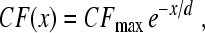 |
5 |
where x is the distance from the base, and CFmax and d are species-dependent parameters representing, respectively, the maximum CF and the “space constant” of the map (i.e., the distance over which the CF decreases by a factor of e). The exponential map implies that for frequencies near CF the interval Δf corresponds to a spatial interval Δx given by Δf/CF ≅ Δx/d. Recognizing that Δf/CF defines the reciprocal of a Q value allows one to rewrite this relation as
 |
6 |
As an example, if Δf is taken as the ERB, then Q is QERB and Δx is the approximate width, or “equivalent rectangular spread” (ERS),12 of the excitation pattern for a pure tone of frequency f = CF (e.g., Garbes 1994).
According to this analysis, the problem of understanding variations in tuning across species is equivalent to that of understanding variations in spatial spread. Perhaps this latter problem admits a simpler solution. For example, Eq. (6) implies that if the cochlear spread of excitation Δx at any given frequency were roughly similar in size across species, then the ratio Q/d would also be similar across species. Taking humans and cats as an example, one would have
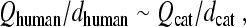 |
7 |
or, equivalently,
 |
8 |
In other words, if the widths of cochlear excitation patterns Δx were more invariant across species than the bandwidths of tuning Δf, then plots of (dhuman/dspecies)Qspecies would be more similar to one another than plots of Qspecies alone.
We test this idea in Figure 15. The figure plots values of (dhuman/dspecies)Qspecies for the four species, cat, guinea pig, chinchilla, and human, using the QERB values from Figure 12 and space constants of the cochlear map (Liberman 1982; Greenwood 1990; Tsuji and Liberman 1997). Comparison with Figure 14A shows that rescaling the QERB values with the factor dhuman/dspecies helps to unify the human and laboratory-animal data. (von Békésy’s measurements, which indicate that both Qelephant and delephant are larger than their human counterparts, imply that rescaling would help bring the elephants back into the fold as well.)
FIG. 15.

Normalizing QERB to compensate for differences in the cochlear map reduces species differences in cochlear tuning. The figure shows values of (dhuman/dspecies)Qspecies for cat, guinea pig, chinchilla, and human computed using the QERB curves from Figure 12 and space constants of the cochlear map.
Under the assumption that the otoacoustic and behavioral values from Figure 12 provide reliable estimates of human tuning, the success of the transformation illustrated in Figure 15 verifies that the spatial spread of excitation (ERS) appears more similar across species than the sharpness of tuning (QERB). Figure 16 shows values of the ERS computed from the QERB values in cat, guinea pig, chinchilla, and human. Panel A shows the ERS on a conventional CF axis; panel B shows the ERS versus CF/CFa|b. [For comparison, direct computation of the ERS for a 16 kHz tone in gerbil using the data of Ren (2002) gives ERS ≅ 0.2–0.3 mm, a value roughly consistent with those in Fig. 16A.] At any given value of the abscissa, the ERS is generally similar in the four species. For example, between-species differences in the ERS are substantially smaller than within-species differences along the length of the BM. The attempt to more closely align comparable regions of the cochlea by plotting the ERS versus CF/CFa|b yields the results shown in panel B. Together, the two transformations involved here—the first converting QERB into the corresponding spread of excitation and the second partially compensating for differences between the base and the apex of the cochlea—nearly unify the tuning data across species. Most noteworthy in the current context: The human spread of excitation—computed from the exceptional estimates of human cochlear tuning shown in Figure 12—appears completely unexceptional.
FIG. 16.

Estimates of the spatial spread of excitation (the ERS, or equivalent rectangular spread) in four species. The curves show values of ERS = d/QERB for cat, guinea pig, chinchilla, and human as computed from the QERB values in Figure 12 and space constants of the cochlear map. Panel (B) shows the ERS plotted vs CF/CFa|b.
The analysis presented here supports the hypothesis that species differences in the sharpness of tuning arise, in large part, because the spatial spread of excitation remains nearly the same at corresponding cochlear locations. (Conversely, if QERB values were to remain the same across species, the ERS would have to differ.) Why might spatial intervals be more invariant across species than frequency tuning? Perhaps the answer is simply that the cochlea is a physical device constructed to operate through the interactions of elements coupled together in space. (The cochlea operates in the spatial domain, not the frequency domain.) Primary among these elements, of course, are the hair cells, which appear spread out in a discrete longitudinal array with a characteristic spacing (∼10 μm) that varies relatively little across species. If the cochlea is built to utilize the spatial interactions of invariant units—whether the interactions be mediated by pressure forces in the surrounding fluid, by fluid flow within the organ of Corti (Karavitaki and Mountain 2007), by mechanical coupling between cells (e.g., Steele et al. 1993; Geisler and Sang 1995; Wen and Boahen 2003), and/or via waves on the tectorial membrane (e.g., Ghaffari et al. 2007)—it is natural to suppose that spatial intervals, such as the widths of excitation patterns or the wavelengths of traveling waves, may be more tightly constrained than derived quantities, such as tuning bandwidths. Recent work supports this view: Mutations that disrupt the longitudinal coupling among the elements, and presumably modify the effective spatial spread of excitation, have pronounced effects on the sharpness of tuning (Russell et al. 2007; Ghaffari et al. 2009).
Our discussion throughout this section has, of course, been speculative. Our purpose has not been to assert that we have found definitive answers to the questions posed, but merely to point out that sharper tuning need not require novel biophysical mechanisms operating in the human cochlea. Large differences in tuning can arise from uncontroversial variations in the cochlear map, as well as from the perhaps apples-with-oranges (apex-with-base) manner in which species have conventionally been compared.
Acknowledgments
We thank Mario Ruggero and Jonathan Siegel for generously sharing their data and for many provocative discussions. We also thank Christopher Bergevin, Paul Fahey, Shirin Farrahi, Jeffery Lichtenhan, Elizabeth Olson, Barbara Shinn-Cunningham, and the two anonymous reviewers for valuable comments on the manuscript. Our work was supported by Grant Nos. R01 DC03687 (CAS), DC00235 (JJG), and DC03909 (AJO) from the NIDCD, National Institutes of Health.
Footnotes
 |
The relationship between SFOAE phase-gradient delays and near-CF group delays found in models of cochlear mechanics depends both on the model’s activity pattern being “tall and broad” and on the spatial pattern of irregularities used in the model (Zweig and Shera 1995; Talmadge et al. 2000). When the irregularity pattern contains spatial-frequency components whose period is near one half the wavelength of the traveling wave at its peak (e.g., if the irregularities arise from cell-to-cell impedance variations that lack significant long-range correlations), then SFOAE delays generally correlate strongly with near-CF BM delays (Zweig and Shera 1995; Shera et al. 2005). If, however, the irregularity pattern is constructed to exclude these spatial frequency components (e.g., Choi et al. 2008), then the proportionality between the two delays can break down.
In previous publications (Shera and Guinan 2003; Shera et al. 2002), we used the term “tuning ratio” to identify the quantity 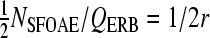 .
.
Because the values of CFa|b in cat, guinea pig, and chinchilla are not all identical, normalizing by CFa|b provides a greater unification of the curves than simply plotting versus CF alone. However, the strongest evidence for the value of normalizing by CFa|b comes from the human data (see “Applications to humans”).
Estimates of CFa|b obtained by aligning the tuning ratios by eye agree closely (i.e., within an eighth of an octave) with estimates derived using more objective procedures (e.g., by approximating the curves by two straight lines that intersect at a point determined by least-squares fitting).
Although the chinchilla NSFOAE trend shows several bends and bumps, the first major deviation from the high-frequency trend occurs near 4 kHz. Other data also identify 4 kHz as the approximate transition between apical-like and basal-like behavior in the chinchilla (e.g., Shera 2007; Temchin et al. 2008).
See footnote †† of Shera et al. (2002).
In principle, the long OAE latencies measured in humans could result from “signal-front delays” rather than from delays associated with mechanical tuning. Frogs, for example, have low-frequency SFOAE delays longer than those in many mammals (Meenderink and Narins 2006; Bergevin et al. 2008) but relatively broad ANF tuning (Ronken 1991). The unusually long latencies observed in the frog are thought to involve mechanisms—perhaps traveling waves on the tectorial curtain of the amphibian papilla (Hillery and Narins 1984)—that contribute little in the way of frequency tuning but add significant mechanical delay. In humans, however, the apparent similarity of human post-mortem BM delays to those in other laboratory animals (Ruggero and Temchin 2007) suggests that there is nothing exceptional about human signal-front delays, and no large additional sources of delay unrelated to tuning have been proposed.
Ruggero and Temchin’s (2007) justification for the assumption that Δτ is similar across species conflates sensitivity with frequency resolution. Although the two often vary together (e.g., in BM velocity transfer functions measured at different intensities at a single location in a given animal or, indeed, in the example of the masses on springs shown in Fig. 3), sensitivity and frequency resolution need not always be simply related, as illustrated by recent measurements in mutant mice (cf., Russell et al. 2007; Ghaffari et al. 2009).
By contrast, the apical–basal changes do affect the tuning ratio, QERB/NSFOAE.
The circumstances of von Békésy’s good fortune are related by Stevens and Warshofsky (1965).
In a scaling-symmetric cochlea, Δx is exactly the equivalent rectangular spread.
Contributor Information
Christopher A. Shera, Email: shera@epl.meei.harvard.edu
John J. Guinan, Jr, Email: jjg@epl.meei.harvard.edu.
Andrew J. Oxenham, Email: oxenham@umn.edu
References
- Banakis R, Cheatham MA, Dallos P, Siegel JH. Spontaneous and tone-evoked otoacoustic emissions in mice. Assoc Res Otolaryngol Abs. 2008;31:195. [Google Scholar]
- Bergevin C, Shera CA (2010) Coherent reflection without traveling waves: on the origin of long-latency otoacoustic emissions in lizards. J Acoust Soc Am 127:2398–2409 [DOI] [PMC free article] [PubMed]
- Bergevin C, Freeman DM, Saunders JC, Shera CA. Otoacoustic emissions in humans, birds, lizards, and frogs: evidence for multiple generation mechanisms. J Comp Physiol A. 2008;194:665–683. doi: 10.1007/s00359-008-0338-y. [DOI] [PMC free article] [PubMed] [Google Scholar]
- Bode H. Network analysis and feedback amplifier design. Princeton: Van Nostrand Reinhold; 1945. [Google Scholar]
- Bredberg G. Cellular patterns and nerve supply of the human organ of Corti. Acta Otolaryngol Suppl. 1968;236:1–135. [PubMed] [Google Scholar]
- Cedolin L, Delgutte B. Pitch of complex tones: rate–place and interspike interval representations in the auditory nerve. J Neurophysiol. 2005;94:347–362. doi: 10.1152/jn.01114.2004. [DOI] [PMC free article] [PubMed] [Google Scholar]
- Choi YS, Lee SY, Parham K, Neely ST, Kim DO. Stimulus-frequency otoacoustic emission: measurements in humans and simulations with an active cochlear model. J Acoust Soc Am. 2008;123:2651–2669. doi: 10.1121/1.2902184. [DOI] [PMC free article] [PubMed] [Google Scholar]
- Cleveland WS. Visualizing data. Summit, NJ: Hobart; 1993. [Google Scholar]
- Cooper NP, Rhode WS. Apical cochlear mechanics: a review of recent observations. In: Palmer AR, Rees A, Summefield AQ, Meddis R, editors. Psychophysical and physiological advances in hearing. London: Whurr; 1997. pp. 11–17. [Google Scholar]
- Dreisbach LE, Siegel JH, Chen W. Stimulus-frequency otoacoustic emissions measured at low and high frequencies in untrained human subjects. Assoc Res Otolaryngol Abs. 1998;21:349. [Google Scholar]
- Eggermont JJ. Wiener and Volterra analyses applied to the auditory system. Hear Res. 1993;66:177–201. doi: 10.1016/0378-5955(93)90139-R. [DOI] [PubMed] [Google Scholar]
- Engström H, Ades HW, Andersson A. Structural pattern of the organ of Corti. Baltimore: Williams and Wilkins; 1966. [Google Scholar]
- Evans EF, Wilson JP. Frequency selectivity in the cochlea. In: Møller AR, Boston P, editors. Basic mechanisms in hearing. New York: Academic; 1973. pp. 519–551. [Google Scholar]
- Garbes PAZ (1994) Evaluating human neural tuning curves from a mechanical model of the cochlea by relating them to psychophysical masking data. PhD thesis, Massachusetts Institute of Technology
- Geisler CD, Sang C. A cochlear model using feed-forward outer-hair-cell forces. Hear Res. 1995;86:132–146. doi: 10.1016/0378-5955(95)00064-B. [DOI] [PubMed] [Google Scholar]
- Ghaffari R, Aranyosi AJ, Freeman DM. Longitudinally propagating traveling waves of the mammalian tectorial membrane. Proc Natl Acad Sci USA. 2007;104:16,510–16,515. doi: 10.1073/pnas.0703665104. [DOI] [PMC free article] [PubMed] [Google Scholar]
- Ghaffari R, Aranyosi AJ, Richardson GP, Freeman DM (2009) Wave upon wave: balancing sensitivity and frequency selectivity of hearing, submitted
- Glasberg BR, Moore BCJ. Derivation of auditory filter shapes from notched-noise data. Hear Res. 1990;47:103–138. doi: 10.1016/0378-5955(90)90170-T. [DOI] [PubMed] [Google Scholar]
- Glasberg BR, Moore BCJ. Frequency selectivity as a function of level and frequency measured with uniformly exciting notched noise. J Acoust Soc Am. 2000;108:2318–2328. doi: 10.1121/1.1315291. [DOI] [PubMed] [Google Scholar]
- Glasberg BR, Moore BCJ, Patterson RD, Nimmo-Smith I. Dynamic range and asymmetry of the auditory filter. J Acoust Soc Am. 1984;76:419–427. doi: 10.1121/1.391584. [DOI] [PubMed] [Google Scholar]
- Goodman SS, Fitzpatrick DF, Ellison JC, Jesteadt W, Keefe DH. High-frequency click-evoked otoacoustic emissions and behavioral thresholds in humans. J Acoust Soc Am. 2009;125:1014–1032. doi: 10.1121/1.3056566. [DOI] [PMC free article] [PubMed] [Google Scholar]
- Greenwood DD. Critical bandwidth and the frequency coordinates of the basilar membrane. J Acoust Soc Am. 1961;33:1344–1356. doi: 10.1121/1.1908437. [DOI] [Google Scholar]
- Greenwood DD. A cochlear frequency-position function for several species—29 years later. J Acoust Soc Am. 1990;87:2592–2605. doi: 10.1121/1.399052. [DOI] [PubMed] [Google Scholar]
- Guinan JJ. Effect of efferent neural activity on cochlear mechanics. Scand Audiol Suppl. 1986;25:53–62. [PubMed] [Google Scholar]
- Guinan JJ, Cooper NP. Medial olivocochlear efferent inhibition of basilar-membrane responses to clicks: evidence for two modes of cochlear mechanical excitation. J Acoust Soc Am. 2008;124:1080–1092. doi: 10.1121/1.2949435. [DOI] [PMC free article] [PubMed] [Google Scholar]
- Guinan JJ, Lin T, Cheng H. Medial-olivocochlear-efferent inhibition of the first peak of auditory-nerve responses: evidence for a new motion within the cochlea. J Acoust Soc Am. 2005;118:2421–2433. doi: 10.1121/1.2017899. [DOI] [PMC free article] [PubMed] [Google Scholar]
- Hartmann WM. Signals, sound, and sensation. Woodbury: AIP; 1997. [Google Scholar]
- Heffner RS, Heffner HE. Hearing in the elephant (Elephas maximus): absolute sensitivity, frequency discrimination, and sound localization. J Comp Physiol Psych. 1982;96:926–944. doi: 10.1037/0735-7036.96.6.926. [DOI] [PubMed] [Google Scholar]
- Hillery CM, Narins PM. Neurophysiological evidence for a traveling wave in the amphibian inner ear. Science. 1984;225:1037–1039. doi: 10.1126/science.6474164. [DOI] [PubMed] [Google Scholar]
- Houtgast T. Psychophysical experiments on ‘tuning curves’ and ‘two-tone inhibition’. Acustica. 1973;29:168–179. [Google Scholar]
- Kalluri R, Shera CA. Comparing stimulus-frequency otoacoustic emissions measured by compression, suppression, and spectral smoothing. J Acoust Soc Am. 2007;122:3562–3575. doi: 10.1121/1.2793604. [DOI] [PubMed] [Google Scholar]
- Kalluri R, Shera CA. Near equivalence of human click-evoked and stimulus-frequency otoacoustic emissions. J Acoust Soc Am. 2007;121:2097–2110. doi: 10.1121/1.2435981. [DOI] [PubMed] [Google Scholar]
- Karavitaki KD, Mountain DC. Evidence for outer hair cell driven oscillatory fluid flow in the tunnel of Corti. Biophys J. 2007;92:3284–3293. doi: 10.1529/biophysj.106.084087. [DOI] [PMC free article] [PubMed] [Google Scholar]
- Kuhn A, Saunders JC. Psychophysical tuning curves in the parakeet: a comparison between simultaneous and forward masking procedures. J Acoust Soc Am. 1980;68:1892–1894. doi: 10.1121/1.385182. [DOI] [Google Scholar]
- Liberman MC. Auditory-nerve response from cats raised in a low-noise chamber. J Acoust Soc Am. 1978;63:442–455. doi: 10.1121/1.381736. [DOI] [PubMed] [Google Scholar]
- Liberman MC. The cochlear frequency map for the cat: labeling auditory-nerve fibers of known characteristic frequency. J Acoust Soc Am. 1982;72:1441–1449. doi: 10.1121/1.388677. [DOI] [PubMed] [Google Scholar]
- Liberman MC, Kiang NYS. Acoustic trauma in cats: cochlear pathology and auditory-nerve activity. Acta Otolaryngol Suppl. 1978;358:1–63. [PubMed] [Google Scholar]
- Lonsbury-Martin BL, Martin GK, Probst R, Coats AC. Spontaneous otoacoustic emissions in the nonhuman primate. II. Cochlear anatomy. Hear Res. 1988;33:69–94. doi: 10.1016/0378-5955(88)90021-4. [DOI] [PubMed] [Google Scholar]
- McGee T, Ryan A, Dallos P. Psychophysical tuning curves of chinchillas. J Acoust Soc Am. 1976;60:1146–1150. doi: 10.1121/1.381216. [DOI] [PubMed] [Google Scholar]
- Meenderink SW, Narins PM. Stimulus frequency otoacoustic emissions in the Northern leopard frog, Rana pipiens pipiens: implications for inner ear mechanics. Hear Res. 2006;220:67–75. doi: 10.1016/j.heares.2006.07.009. [DOI] [PubMed] [Google Scholar]
- Moore BCJ. Psychophysical tuning curves measured in simultaneous and forward masking. J Acoust Soc Am. 1978;63:524–532. doi: 10.1121/1.381752. [DOI] [PubMed] [Google Scholar]
- Moore BCJ, Glasberg BR. Auditory filter shapes derived in simultaneous and forward masking. J Acoust Soc Am. 1981;70:1003–1014. doi: 10.1121/1.386950. [DOI] [PubMed] [Google Scholar]
- Moore BCJ, Glasberg BR, Roberts B. Refining the measurement of psychophysical tuning curves. J Acoust Soc Am. 1984;76:1057–1066. doi: 10.1121/1.391425. [DOI] [PubMed] [Google Scholar]
- Neff DL. Stimulus parameters governing confusion effects in forward masking. J Acoust Soc Am. 1985;78:1966–1976. doi: 10.1121/1.392653. [DOI] [PubMed] [Google Scholar]
- Nowotny M, Gummer AW. Nanomechanics of the subtectorial space caused by electromechanics of cochlear outer hair cells. Proc Natl Acad Sci USA. 2006;103:2120–2125. doi: 10.1073/pnas.0511125103. [DOI] [PMC free article] [PubMed] [Google Scholar]
- O’Loughlin BJ, Moore BCJ. Improving psychoacoustical tuning curves. Hear Res. 1981;5:343–346. doi: 10.1016/0378-5955(81)90057-5. [DOI] [PubMed] [Google Scholar]
- Oxenham AJ, Dau T. Towards a measure of auditory-filter phase response. J Acoust Soc Am. 2001;110:3169–3178. doi: 10.1121/1.1414706. [DOI] [PubMed] [Google Scholar]
- Oxenham AJ, Shera CA. Estimates of human cochlear tuning at low levels using forward and simultaneous masking. J Assoc Res Otolaryngol. 2003;4:541–554. doi: 10.1007/s10162-002-3058-y. [DOI] [PMC free article] [PubMed] [Google Scholar]
- Papoulis A. The Fourier integral and its applications. New York: McGraw-Hill; 1962. [Google Scholar]
- Patterson RD. Auditory filter shapes derived with noise stimuli. J Acoust Soc Am. 1976;59:640–654. doi: 10.1121/1.380914. [DOI] [PubMed] [Google Scholar]
- Patterson RD, Nimmo-Smith I, Weber DL, Milroy R. The deterioration of hearing with age: frequency selectivity, the critical ratio, the audiogram, and speech threshold. J Acoust Soc Am. 1982;72:1788–1803. doi: 10.1121/1.388652. [DOI] [PubMed] [Google Scholar]
- Recio-Spinoso A, Temchin AN, Dijk P, Fan YH, Ruggero MA. Wiener-kernel analysis of responses to noise of chinchilla. J Neurophysiol. 2005;93:3615–3634. doi: 10.1152/jn.00882.2004. [DOI] [PubMed] [Google Scholar]
- Ren T. Longitudinal pattern of basilar membrane vibration in the sensitive cochlea. Proc Natl Acad Sci USA. 2002;99:17,101–17,106. doi: 10.1073/pnas.262663699. [DOI] [PMC free article] [PubMed] [Google Scholar]
- Ronken DA. Spike discharge properties that are related to the characteristic frequency of single units in the frog auditory nerve. J Acoust Soc Am. 1991;90:2428–2440. doi: 10.1121/1.402047. [DOI] [PubMed] [Google Scholar]
- Rosen SR, Baker RJ, Darling A. Auditory filter nonlinearity at 2 kHz in normal hearing listener. J Acoust Soc Am. 1998;103:2539–2350. doi: 10.1121/1.422775. [DOI] [PubMed] [Google Scholar]
- Ruggero MA, Rich NC. Chinchilla auditory-nerve responses to low-frequency tones. J Acoust Soc Am. 1983;73:2096–2108. doi: 10.1121/1.389577. [DOI] [PubMed] [Google Scholar]
- Ruggero MA, Temchin AN. Unexceptional sharpness of frequency tuning in the human cochlea. Proc Natl Acad Sci USA. 2005;102:18,614–18,619. doi: 10.1073/pnas.0509323102. [DOI] [PMC free article] [PubMed] [Google Scholar]
- Ruggero MA, Temchin AN. Similarity of traveling-wave delays in the hearing organs of humans and other tetrapods. J Assoc Res Otolaryngol. 2007;8:153–166. doi: 10.1007/s10162-007-0081-z. [DOI] [PMC free article] [PubMed] [Google Scholar]
- Ruggero MA, Rich NC, Robles L, Shivapuja BG. Middle-ear response in the chinchilla and its relationship to mechanics at the base of the cochlea. J Acoust Soc Am. 1990;87:1612–1629. doi: 10.1121/1.399409. [DOI] [PMC free article] [PubMed] [Google Scholar]
- Russell IJ, Legan PK, Lukashkina VA, Lukashkin AN, Goodyear RJ, Richardson GP. Sharpened cochlear tuning in a mouse with a genetically modified tectorial membrane. Nat Neurosci. 2007;10:215–223. doi: 10.1038/nn1828. [DOI] [PMC free article] [PubMed] [Google Scholar]
- Salt AN (2001) Cochlear fluids simulator v1.6h, (http://oto.wustl.edu/cochlea/model.htm, downloaded 1 Dec. 2005)
- Schairer KS, Ellison JC, Fitzpatrick D, Keefe DH. Use of stimulus-frequency otoacoustic emission latency and level to investigate cochlear mechanics. J Acoust Soc Am. 2006;120:901–914. doi: 10.1121/1.2214147. [DOI] [PMC free article] [PubMed] [Google Scholar]
- Serafin JV, Moody DB, Stebbins WC. Frequency selectivity of the monkey’s auditory system: psychophysical tuning curves. J Acoust Soc Am. 1982;71:1513–1518. doi: 10.1121/1.387851. [DOI] [PubMed] [Google Scholar]
- Shera CA. Mammalian spontaneous otoacoustic emissions are amplitude-stabilized cochlear standing waves. J Acoust Soc Am. 2003;114:244–262. doi: 10.1121/1.1575750. [DOI] [PubMed] [Google Scholar]
- Shera CA. Laser amplification with a twist: traveling-wave propagation and gain functions from throughout the cochlea. J Acoust Soc Am. 2007;122:2738–2758. doi: 10.1121/1.2783205. [DOI] [PubMed] [Google Scholar]
- Shera CA, Guinan JJ. Stimulus-frequency-emission group delay: a test of coherent reflection filtering and a window on cochlear tuning. J Acoust Soc Am. 2003;113:2762–2772. doi: 10.1121/1.1557211. [DOI] [PubMed] [Google Scholar]
- Shera CA, Zweig G. Order from chaos: resolving the paradox of periodicity in evoked otoacoustic emission. In: Duifhuis H, Horst JW, Dijk P, Netten SM, editors. Biophysics of hair cell sensory systems. Singapore: World Scientific; 1993. pp. 54–63. [Google Scholar]
- Shera CA, Guinan JJ, Oxenham AJ. Revised estimates of human cochlear tuning from otoacoustic and behavioral measurements. Proc Natl Acad Sci U S A. 2002;99:3318–3323. doi: 10.1073/pnas.032675099. [DOI] [PMC free article] [PubMed] [Google Scholar]
- Shera CA, Tubis A, Talmadge CL. Coherent reflection in a two-dimensional cochlea: short-wave versus long-wave scattering in the generation of reflection-source otoacoustic emissions. J Acoust Soc Am. 2005;118:287–313. doi: 10.1121/1.1895025. [DOI] [PubMed] [Google Scholar]
- Shera CA, Tubis A, Talmadge CL. Testing coherent reflection in chinchilla: auditory-nerve responses predict stimulus-frequency emissions. J Acoust Soc Am. 2008;124:381–395. doi: 10.1121/1.2917805. [DOI] [PMC free article] [PubMed] [Google Scholar]
- Siegel JH, Temchin AN, Ruggero MA. Empirical estimates of the spatial origin of stimulus-frequency otoacoustic emissions. Assoc Res Otolaryngol Abs. 2003;26:679. [Google Scholar]
- Siegel JH, Cerka AJ, Temchin AN, Ruggero MA. Similar two-tone suppression patterns in SFOAEs and the cochlear microphonics indicate comparable spatial summation of underlying generators. Assoc Res Otolaryngol Abs. 2004;27:539. [Google Scholar]
- Siegel JH, Cerka AJ, Recio-Spinoso A, Temchin AN, Dijk P, Ruggero MA. Delays of stimulus-frequency otoacoustic emissions and cochlear vibrations contradict the theory of coherent reflection filtering. J Acoust Soc Am. 2005;118:2434–2443. doi: 10.1121/1.2005867. [DOI] [PubMed] [Google Scholar]
- Sisto R, Moleti A. Transient evoked otoacoustic emission latency and cochlear tuning at different stimulus levels. J Acoust Soc Am. 2007;122:2183–2190. doi: 10.1121/1.2769981. [DOI] [PubMed] [Google Scholar]
- Songer JE, Rosowski JJ. Transmission matrix analysis of the chinchilla middle ear. J Acoust Soc Am. 2007;122:932–942. doi: 10.1121/1.2747157. [DOI] [PMC free article] [PubMed] [Google Scholar]
- Steele CR, Baker G, Tolomeo J, Zetes D. Electro-mechanical models of the outer hair cell. In: Duifhuis H, Horst JW, Dijk P, Netten SM, editors. Biophysics of hair cell sensory systems. Singapore: World Scientific; 1993. pp. 207–214. [Google Scholar]
- Stevens SS, Warshofsky F. Sound and hearing. New York: Time-Life Books; 1965. [Google Scholar]
- Talmadge CL, Tubis A, Long GR, Piskorski P. Modeling otoacoustic emission and hearing threshold fine structures. J Acoust Soc Am. 1998;104:1517–1543. doi: 10.1121/1.424364. [DOI] [PubMed] [Google Scholar]
- Talmadge CL, Tubis A, Long GR, Tong C. Modeling the combined effects of basilar membrane nonlinearity and roughness on stimulus frequency otoacoustic emission fine structure. J Acoust Soc Am. 2000;108:2911–2932. doi: 10.1121/1.1321012. [DOI] [PubMed] [Google Scholar]
- Temchin AN, Recio-Spinoso A, Dijk P, Ruggero MA. Wiener kernels of chinchilla auditory-nerve fibers: verification using responses to tones, clicks, and noise and comparison with basilar-membrane vibrations. J Neurophysiol. 2005;93:3635–3648. doi: 10.1152/jn.00885.2004. [DOI] [PMC free article] [PubMed] [Google Scholar]
- Temchin AN, Rich NC, Ruggero MA. Threshold tuning curves of chinchilla auditory-nerve fibers. I. Dependence on characteristic frequency and relation to the magnitudes of cochlear vibrations. J Neurophysiol. 2008;100:2889–2898. doi: 10.1152/jn.90637.2008. [DOI] [PMC free article] [PubMed] [Google Scholar]
- Tsuji J, Liberman MC. Intracellular labeling of auditory nerve fibers in guinea pig: central and peripheral projections. J Comp Neurol. 1997;381:188–202. doi: 10.1002/(SICI)1096-9861(19970505)381:2<188::AID-CNE6>3.0.CO;2-#. [DOI] [PubMed] [Google Scholar]
- Békésy G. Experiments in hearing. New York: McGraw-Hill; 1960. [Google Scholar]
- Wen B, Boahen KA. A linear cochlear model with active bi-directional coupling. Proc 25th Ann Int Conf IEEE Eng Med Biol Soc. 2003;3:2013–2016. [Google Scholar]
- Wright AA. Dimensions of the cochlear stereocilia in man and in guinea pig. Hear Res. 1984;13:89–98. doi: 10.1016/0378-5955(84)90099-6. [DOI] [PubMed] [Google Scholar]
- Zweig G, Shera CA. The origin of periodicity in the spectrum of evoked otoacoustic emissions. J Acoust Soc Am. 1995;98:2018–2047. doi: 10.1121/1.413320. [DOI] [PubMed] [Google Scholar]