Trait Variability of Cancer Cells Quantified by High-Content Automated Microscopy of Single Cells

Abstract

Mapping quantitative cell traits (QCT) to underlying molecular defects is a central challenge in cancer research because heterogeneity at all biological scales, from genes to cells to populations, is recognized as the main driver of cancer progression and treatment resistance. A major roadblock to a multiscale framework linking cell to signaling to genetic cancer heterogeneity is the dearth of large-scale, single-cell data on QCT-such as proliferation, death sensitivity, motility, metabolism, and other hallmarks of cancer. High-volume single-cell data can be used to represent cell-to-cell genetic and nongenetic QCT variability in cancer cell populations as averages, distributions, and statistical subpopulations. By matching the abundance of available data on cancer genetic and molecular variability, QCT data should enable quantitative mapping of phenotype to genotype in cancer. This challenge is being met by high-content automated microscopy (HCAM), based on the convergence of several technologies including computerized microscopy, image processing, computation, and heterogeneity science. In this chapter, we describe an HCAM workflow that can be set up in a medium size interdisciplinary laboratory, and its application to produce high-throughput QCT data for cancer cell motility and proliferation. This type of data is ideally suited to populate cell-scale computational and mathematical models of cancer progression for quantitatively and predictively evaluating cancer drug discovery and treatment.

1. Introduction

Cancer cells both across and within individual patients are heterogeneous with respect to genetic (and epigenetic) makeup (Heng et al., 2009). Furthermore, it is increasingly appreciated that even within genetically identical clonal cell populations, individual cells may differ from each other in phenotypic traits (Brock et al., 2009; Stockholm et al., 2007). Genetic and nongenetic heterogeneity remain a formidable challenge for cancer treatment, especially in the case of molecular targeted drugs. Large-scale genetic and epigenetic analyses of cancer variability have begun to extract common patterns at the molecular scale within this morass of heterogeneity.

More recently, powerful cell phenotype analytical methods are coming on line, mostly due to the convergence of image processing, computer-driven automation and high-throughput microscopes (Dove, 2003; Evans and Matsudaira, 2007; Perlman et al., 2004; Starkuviene and Pepperkok, 2007). These methods, termed for convenience high-content automated microscopy (HCAM), enable large-scale analyses of cancer cell phenotype variability that will eventually match the scope of genetic variability analyses.

In this chapter, we describe our implementation of HCAM methods in order to quantify cell traits such as proliferation and motility, and their variability within a cell population such as a cancer cell line. To be clear, we refer to a quantitative cell trait (QCT) as a cell-scale functional property (e.g., proliferation, motility, metabolism, death sensitivity) that displays cell-to-cell variability in a cell population, with respect to some quantitative metric. It is highly desirable that a QCT be defined in numeric terms for machine compatibility, since it is virtually impossible to intuitively deal with, follow in time, or predict consequences of QCT combinations, for example, in cancer progression or drug response. In these early days, these metrics are not firmly established and undoubtedly at some point will have to be agreed upon, particularly for comparing data from different sources in an automated fashion.

In this chapter, our primary goal was to describe methods that define QCT heterogeneity quantitatively, regardless of the source of heterogeneity (e.g., genetic, epigenetic, nongenetic). However, we recognize that, once metrics are established, investigating the source of QCT variability becomes a tantalizing priority. Such investigations may span from identification of molecular mechanisms responsible for generating or dampening QCT variability, to mathematical or statistical modeling for best guess of the type of heterogeneity source (e.g., genetic or nongenetic). Consequences are very practical, because in the case of genetic sources one would expect permanent inheritance of the heterogeneity source, whereas a nongenetic source would produce temporary inheritance of heterogeneity.

2. Background

Heterogeneity is a central feature of cancer that occurs at all biological scales, from genes to cells to populations. For decades, it has been suspected to be largely responsible for cancer progression and resistance to treatment, spawning intense studies especially at the genetic and molecular level. For example, panels of cancer cell lines have been subjected to genomic, gene expression or protein array analyses, evidencing a large number of genetic mutations, and signaling network alterations associated with malignant transformation. While these studies have been enormously informative and have taken our understanding of cancer to incredible depth, they have suffered from at least two limitations: (i) high-throughput genetic and biochemical studies are generally impractical at the single-cell level and are mostly based on average measurements of a test cell population; and (ii) genotype to phenotype mapping in a single cell, that is, linking genetic or molecular changes with phenotypic trait output (like motility or proliferation) remains challenging. These limitations are especially frustrating in the context of cancer progression, which is paced by the appearance of cell clones abnormal with respect to “hallmark” traits, such that cancer may be referred to as a disease of outliers. Methods to map QCT to underlying molecular defects would effectively produce a multiscale bridge from cancer genetics to cancer cell biology. In this multiscale framework, treatment and drug discovery could be approached with predictive methods.

Analysis at the single-cell level of QCT variability, regardless of source, is commanding increasing attention due to convergent advances in several disciplines. As a whole, the science of heterogeneity has reached maturity in many fields, such as face recognition, machine learning, and signal processing, producing theory that is applicable to cancer cell biology, as well as a wealth of mathematical and computational tools. Computer-driven microscopes are rapidly being refined and promise to deliver for adherent cells the spectacular advances flow cytometry has produced for cells in suspension. Image processing software and automation have the potential to create automated workflows to capture and analyze the behavior of thousands of single cells under tens of conditions in relatively short experimental times.

This ensemble of technology is commonly referred to as HCAM. Its application to cancer cell biology promises to revolutionize our understanding of cell-to-cell variability with respect to a phenotypic trait, referred to above as QCT. It is perhaps worth noting that QCT studies are gaining traction in fields other than cancer. An emerging view is that phenotypic trait variability is inherent to living systems, in large part as an inevitable consequence of biological “noise” at several steps of intracellular molecular operation (e.g., gene transcription, mRNA translation, protein folding). Furthermore, local microenvironmental conditions may extinguish or amplify this noise and, to an extent, even nongenetic variability is inherited from mother to daughter cells on a temporary basis. Normal cells apply considerable resources to constrain or dampen both genetic and nongenetic variability of their traits, particularly as they become functional components of differentiated tissues. In this sense, variability is a negative factor with respect to homeostasis. However, trait variability may provide options to cells for responding to microenvironmental changes, for example, by pushing operation of that trait to the extremes of a range in order to survive under extreme microenvironmental stress, and perhaps for evolving new strategies. In summary, variability of a phenotypic cell trait can be considered a measure of cell adaptability, as well as of evolvability of underlying biochemical circuitry. From this broader perspective, an intriguing view is that during cancer progression the adaptability of cancer cells to microenvironmental changes is ever-increasing. QCT analysis is a key step to breaking down adaptability into numerical parameters that can be evaluated spatially and temporally by higher scale computational modeling.

3. Experimental and Computational Workflow

Advances in experimental and microscopic technologies have made it possible to gather high-quality high-content images of cells and cellular components at an ever-increasing rate. Development of such state-of-the-art equipment and tools allows investigators to gather spatial (i.e., in x-, y-, and z-axes, covering many fields of view, using multiple wavelengths) and time-resolved (i.e., at rapid intervals, over several days) quantifiers that describe various cell traits (i.e., motility, proliferation) in vitro. Such methodology can also be used to explore heterogeneity of traits of individual cells within cell populations.

HCAM is rapidly becoming the most efficient methodology to measure phenotypic traits of cancer cell populations at the single-cell level. In this section, we describe a streamlined workflow for acquiring and processing HCAM data that we have established for our own group (Fig. 2.1). This process can be divided into the key steps highlighted in Fig. 2.1. For some of these steps, recent comprehensive reviews have appeared and the reader is referred to those after a brief discussion. Other steps are dealt with in detail. In brief, the workflow is enabled by development of an informatics pipeline for images and image-associated metadata. Image features are derived using a suite of existing and newly developed image analysis and computer software tools. Ultimately, the goal of this workflow is to establish an efficient pipeline to store, disseminate, and analyze single-cell data for streamlining the use of data categories, for example, for input into mathematical/computational models (Fig. 2.1).

Figure 2.1.

Workflow for computer-assisted analysis of quantitative cell traits (QCT). For simplification, the general workflow associated with measuring QCT is broken into the following steps: (i) time-lapse image acquisition (e.g., assay setup, microscopy); (ii) data management (OME, ACCRE); (iii) image processing (e.g., cell identification, segmentation, tracking); (iv) cellular parameter extraction (e.g., cell speed, doubling time); (v) statistical analysis ((non)parametric tests); and (vi) data categories (i.e., averages, distributions, and “statistical subpopulations”)

For simplification, the workflow has been broken down into the following steps (all of which are expanded upon in the following sections):

1. Time-lapse image acquisition

2. Data management

3. Image processing (segmentation and tracking)

4. Cellular parameter extraction

5. Statistical analyses

6. Data categories (average, distribution, statistical subpopulations)

3.1. Time-lapse image acquisition

Measurement of spatially- and time-resolved phenotypic traits involves large-scale data acquisition. In order to examine traits efficiently in many cell lines, in many relevant conditions (e.g., hypoxia, drug treatment), and over time, inclusion of a high-throughput methodology such as HCAM is vital. We have primarily utilized a temperature- and CO₂-controlled, automated, spinning-disk confocal microscope, the BD Pathway 855 (BD Biosciences, Rockville, MD) for single-cell phenotypic studies, although many other systems exist that provide similar functions. The Bioimager is capable of imaging an entire 96-well microplate in a single channel and focal plane in 10 min, but also has the flexibility to accommodate many other sample formats. Imaging can also be performed repeatedly with multiple images per well, multiple focal planes (z-sections), and using multiple fluorescent channels (using two light sources and various filters for a variety of fluorophores), making the setup ideal for performance of high-content time-lapse studies. In addition, the machine has a capacity for automated liquid handling allowing for precise control of the duration and volume of compound treatments. Lastly, this machine is versatile with adaptable hardware that is directly integrated into our data management system (described below in detail). Ultimately, increasing the efficiency of data acquisition via implementation of such methodology makes it possible to maximize the amount (and potentially the value) of quantitative data extracted from image-based single-cell studies.

There are several trade-offs that require careful consideration during single-cell studies. First, the speed at which images can be acquired limits the number of wells, surface area covered, number of channels, or z-sections, etc. that can be imaged prior to returning to the starting position for the next sequential round of image acquisition. For instance, the frequency of image acquisition is of critical importance when examining motile cells. In order to automate the identification and tracking of individual cells over time (repeated images), the distance the cell has moved between frames must be kept below a minimal threshold that is dependent on the density of cells imaged. It is computationally more challenging to identify a cell between two sequential images as the number of cells and the distance a cell moves increase. A list of imaging trade-offs is shown in Table 2.1.

Table 2.1.

Imaging trade-offs for dynamic high-content automated microscopy

Frequency of image acquisition

Automatic tracking algorithms become more error-prone as cell speed or time between successive frames increases

Increasing imaging frequency facilitates automatic tracking but increases total light exposure, which increases risk of phototoxicity and photobleaching

Duration of light exposure

Increasing exposure time increases signal-to-noise ratio, but also increases total light exposure, which increases risk of phototoxicity and photobleaching

Minimum exposure time that provides sufficient signal-to-noise ratio over the entire experiment should be employed

Camera binning may be used to increase signal at the cost of some spatial resolution

Area to be imaged

Directly determines the maximum number of cells to be imaged

Decreasing objective magnification (e.g., from 203 to 103) increases area but reduces resolution

Digital stitching of adjacent frames (montaging) can be used to increase imaged area at the cost of time, file size, and increased light exposure at overlapping frame borders

Number of channels and z-sections

Increasing number of parameters and z-sections increases light exposure and time required per well

Number of conditions and cell types and technical replicates

Limited by the frequency of imaging required in each well to address biological question and time required to image each well

Increasing technical replicates allows sufficient number of cells to be imaged if low density culture is required initially

Duration of experiment

Automatic tracking algorithms become more error-prone as cell density increases, which occurs exponentially under optimal culture conditions

Longer experiment times may affect maintenance microenvironmental conditions (e.g., depletion of nutrients, medium evaporation, etc.)

Another important consideration is photobleaching and phototoxicity. This is generally not a problem for phase-contrast imaging, but can be a substantial limitation for fluorescence imaging. Nipkow spinning disk confocal imaging is particularly well suited for reducing phototoxicity and photobleaching and has become the method of choice for live-cell imaging (Gräf et al., 2005). However, a limitation of imaging through spinning disks is that z-axis resolution is reduced compared to that of laser scanning confocal imaging. Regardless of whether spinning disks are used, the potential effects of imaging on cellular phenotypes must be considered.

3.2. Data management

Individual HCAM experiments generate large datasets, commonly exceeding 50 GB in size. Therefore, data management—including storage, retrieval, backup, and processing—is facilitated by incorporation of data into the open microscopy environment (OME; http://www.openmicroscopy.org; Swedlow et al., 2003). This open-source software has been designed specifically to address the challenges of HCAM data and provides a standardized management platform by developing software and data format standards for the storage and manipulation of biological microscopy data (Goldberg et al., 2005; Swedlow et al., 2009). OME has previously been used in a number of biological studies to examine many aspects of cellular behavior (Dikovskaya et al., 2007; Porter et al., 2007). An OME remote objects (OMERO) server is established, which provides access to image data (the binary pixel data) and metadata (i.e., associated information about instrument settings, configurations, annotations). Access to data is enabled through client applications that simply run on a user’s computer. These include light-weight web-based interfaces, which can be accessed from any computer with a standard web browser; Java-based client applications, which provide more functionality than the web interface, but must be installed separately on each client computer; and a full cross-platform API, which provides data accessibility from third-party applications like ImageJ and VisBio. In addition, incorporation of data into OME provides MATLAB bindings to facilitate sophisticated image processing and analysis directly through the OMERO server.

3.3. Image processing

Formatted images classified into datasets are then processed using various image analysis tools/algorithms (e.g., cell tracking, segmentation); we use a combination of some existing and freely available from open sources such as MetaMorph^™ (Molecular Devices, Sunnyvale, CA), ImageJ (http://rsbweb.nih.gov/ij/; Rasband, 1997–2006), CellProfiler (http://www.cellprofiler.org; Carpenter et al., 2006), OpenLab (Improvision, Waltham, MA), and others custom-developed in-house, to utilize the Vanderbilt Advanced Computing Center for Research & Education (ACCRE) Cluster for rapid processing of individual wells in parallel. MATLAB and Unix Shell scripts, which are designed to run in a high-throughput mode, facilitate this effort. We will present three specific processing modules that were custom-designed for processing of cell motility (Section 4.1) and proliferation (Section 4.2).

3.4. Cellular parameter extraction

The output from the image processing pipeline is a set of cell parameters and images for visual inspection. Information from each tracked cell can be extracted from raw or processed images or from aggregate data for further data analysis. Typical parameters obtained from each image include cell perimeter, mean pixel intensity, and measures of shape such as eccentricity and solidity. Other measurements first require the identification of individual cells across multiple frames. These QCT include parameters of cell motility (e.g., speed, direction), intermitotic times (IMT), and progeny trees. Once all data are extracted from images, it is saved as a set of CSV files for statistical analysis and a set of images for visual inspection (i.e., quality control).

3.5. Statistical analysis

A variety of analytical and statistical tools are applied to further analyze single-cell data, using a few statistical/mathematical packages including, R (http://www.r-project.org/; free software environment), SPSS (SPSS, Inc., Chicago, IL), and Mathematica (Wolfram Research, Inc., Champaign, IL).

Averages and distributions of data are tested using a combination of parametric and nonparametric statistical tests, as needed. First, normality of data is tested using various statistical tests (e.g., D’ Agostino’s K-squared, Shapiro Wilks W), dependent upon sample size, prior to all further analyses. Given a dataset that classically fits normality, parametric statistics (e.g., Student’s t-test, ANOVA) can be applied to detect significant relationships, and presentation of averages, standard deviation (SD), and standard error (SE) is sufficient to describe the population. However, given nonnormality, slightly more extraneous nonparametric tests must be employed to accurately capture population dynamics (e.g., Wilcoxon signed-rank, Kolmogorov–Smirnov tests). Of note, failure to verify assumptions about data (particularly in the study of population heterogeneity) can lead to unfortunate misinterpretation and wrongful conclusions.

Statistical subpopulation analysis will also employ a number of other classic and adapted methods, which are described at length in Section 3.6.1.

3.6. Data categories

Raw or processed data can be presented in various ways, of which we discuss three: (i) averages, (ii) distributions, or (iii) “statistical subpopulations” (i.e., variability distribution discretized by statistical techniques such as clustering). Each of these categories can then be incorporated into corresponding mathematical models.

3.6.1. Averages

We have previously incorporated average data, for various phenotypic traits for a panel of genetically related breast cancer cells into the hybrid-discrete continuum (HDC) mathematical model for parameterization (Anderson et al., 2009). However, with the realization of heterogeneity of cell populations, presentation of a single value (average) is often inadequate for an accurate description. Although SD or SE can sometimes be used to effectively describe the variability of normal (Gaussian) populations, skewed nonnormal datasets rich with outliers and possible subpopulations should not rely on these means. Instead, analysis of population probability distributions and subpopulations via various approaches is preferable in these instances, as described below.

3.6.2. Distributions

Obtaining single-cell measures using HCAM, in combination with rigorous statistical treatment, allows examination and analysis of large populations of cells (N > 1000) in a fairly efficient manner. Using this type of data acquisition for phenotypic traits, in lieu of population-based metrics, allows for presentation of probability distribution, which describes both the range of possible values that a random variable can attain and the probability that the value is within any subset of that range. This category of measurement is particularly useful for representing the spread or variability (i.e., heterogeneity) of a cell population by depicting the nuances of its data (e.g., non-normality, skewness, kurtosis, outliers), which are lost using simple presentation of averages. By providing such data for parameterization of mathematical and computational models where appropriate, one can model heterogeneity of populations more realistically (in line with experimentation), which may ultimately lead to important insights otherwise overlooked. A specific example of applying these techniques to single-cell motility data is detailed below in Section 4.1.

3.6.3. Statistical subpopulations

Using other statistical approaches, raw data for various phenotypic cell traits can also be processed to reveal “subpopulations” present within the greater population being examined. In order to quantify intracell line variability, we discretize the continuous distribution measurements described in the above section into “functional subpopulations,” as previously described (Loo et al., 2007; Perlman et al., 2004; Slack et al., 2008). The advantage of identifying discrete subpopulations is that they can be compared across cell lines and identify common trends in response to perturbations of interest. Specifically, methods can be employed to estimate trait subpopulations using model-fit criteria, such as Bayesian information criterion (BIC) or gap statistics (Fraley and Raftery, 2002). BIC is an approximation of integrated likelihood, according to Eq. (2.1):

$$2log(p(D\mid M_k))\approx 2log(p(D\mid {\widehat{\theta }}_k,M_k))-v_{k}log(n)={\text{BIC}}_k$$ (2.1)

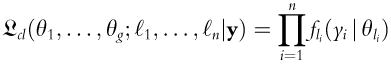
v_k is the number of independent parameters to be estimated in model M_k. θ_k is the parameter being estimated, and n is the number of points in the dataset D. This approximation has been shown to be a consistent estimator of density, even when dealing with nonparametric (Roeder and Wasserman, 1995) or noisy data. Expectation maximization (EM) is also used in statistics for finding maximum likelihood estimates (MLE) of parameters with a known number of clusters (Eliason, 1993). Using this method, model-based hierarchical agglomerative clustering is used to compute an approximate maximum for the classification likelihood, following Eq. (2.2), as previously described (Fraley and Raftery, 2002):

(2.2)

ℓ_n labels a unique classification of each observation, and θ_g is the parameter estimate for each cluster. By combining the hierarchical agglomerative clustering with both EM and BIC, a robust strategy is developed. The brief outline of this algorithm is as follows: (1) choose maximum number of clusters; (2) perform hierarchical agglomerative clustering to estimate a classification for the data under each model, up to a selected maximum number; (3) compute the EM to determine parameters under each model; and (4) utilize BIC to select which is the most likely model of the data.

Additional statistical techniques (i.e., principal components analysis (PCA) or Gaussian mixed models (GMM)) can then be applied as needed to reduce the dimension of a dataset and to find clusters of cells or sub-populations. Ultimately, these subpopulations are represented as probabilistic mixtures of stereotypes (i.e., phenotypes). As presented previously (Loo et al., 2007; Perlman et al., 2004; Slack et al., 2008), we can summarize the percentages of states within a cancer population as a “subpopulation trait profile”—a simple probability vector whose entries sum to one. This analysis allows us to approximate subpopulations (i.e., heterogeneity) that exist within a cell line population with respect to a specific cell trait. Further, we can also use this approach to examine whether specific microenvironmental perturbations (e.g., hypoxia, drug treatment) influence/induce apparent patterns of heterogeneity of cancer cell populations. This particular approach can be invaluable for explaining shifts of cell populations, or more interestingly cell subpopulations, which is quickly becoming a major field of study in cancer research.

These analyses have all been previously used in different combinations for teasing apart cell subtypes based on various parameters (Loo et al., 2007; Perlman et al., 2004; Slack et al., 2008). In summary, this is just one approach for numerically describing the heterogeneity of cell populations, particularly highlighting outliers, based on any number of relevant traits of interest. Much like flow cytometry separates a cell population from suspension into various subpopulations based on certain assignments (e.g., fluorescent marker, cell size), the coupling of HCAM and rigorous statistical tests can provide a means for separating or grouping of live cells dynamically over time from image-based studies. A specific example of applying these techniques to single-cell proliferation data is detailed below in Section 4.2.

4. Application to Traits Relevant to Cancer Progression

As described above, various experimental and computational tools are being developed to investigate a number of applications relevant to the study of QCT in cancer progression. In this chapter, we have focused on measurement and analysis of two specific phenotypic traits (QCT) of single cells, motility and proliferation, both of which are hallmarks of cancer (Hanahan and Weinberg, 2000). It is well established that both traits are aberrantly regulated during disease progression, and probable that intervention strategies targeting these processes may be useful in clinical treatment. The following sections briefly expand upon the clinical importance of each trait, our chosen methodology for various analyses of each, and the implications of conducting such studies.

4.1. Cell motility

Cell motility plays an essential role in many biological systems, but precise quantitative knowledge of the biophysical processes involved in cell migration is limited. It is well established that migration of both epithelial and transformed cancer cells is a complex and dynamic process, which involves changes in cell size, shape, and overall movement (Friedl and Wolf, 2003). Therefore, one can characterize cell motility by quantifying several metrics. This provides opportunities to improve the predictive accuracy of computational and mathematical models by incorporating more numerical parameters. Herein, we present a method for assessing single-cell motility, combining experimental, statistical and computational tools, and apply it to the analysis of the dynamics of “unbiased” single-cell migration in vitro (i.e., undirected, or without addition of chemoattractant). This pipeline for analysis was designed with the intention of examining large numbers of heterogeneous cancer cell populations (i.e., cell lines in vitro). This method improves upon classic methods for studying migration (e.g., Boyden chamber) because it captures single-cell dynamics underlying the heterogeneity of cancer cell populations.

4.1.1. Single-cell motility analysis: image acquisition and validation

We established protocols for both manual (Harris et al., 2008) and automated (custom-written algorithms) cell tracking of single-cell motility. Manual cell tracking is standard practice (Harris et al., 2008) and not covered in this chapter. Although facilitated by several software packages and image analysis tools (Section 3.3), it is laborious and time-consuming (Harris et al., 2008) and limits the throughput. In the context of HCAM and high-throughput studies, it still has a critical function to validate automated analyses.

Automated high-throughput cell tracking (thousands of cells) presents significant challenges, discussed in the following. Due to low signal-to-noise ratio (low contrast between cell and background), automated cell tracking of digital bright-field or phase-contrast microscopic images is often impractical and error prone. Fluorescent-based imaging has far superior signal-to-noise ratios and the resultant images significantly simplify the process of automated tracking. Therefore, for high-throughput studies in our laboratory (using the BD 855 Pathway), cells are labeled with a nuclear protein (histone H2B) conjugated to monomeric red fluorescent protein (H2BmRFP; Addgene Plasmid 18982) to enable identification of nuclei of individual cells. This protein has been used by many groups for imaging purposes, and to date no significant alterations in cellular function due to its expression have been described. The most efficient method for obtaining pooled populations of cells with stable expression of a transgene is using retroviral-mediated transduction, although any method that produces similar results may be employed alternatively. Cells should be flow-sorted to minimize the number of nonexpressing cells within the populations. Numerous protocols exist for these procedures and will not be covered here further. Once a stable cell line is established in which the fluorescent protein is expressed, various parameters must be compared to the parental strain to ensure no obvious clonal selection has occurred. HCAM assays can then be carried out as follows: (1) Cells are seeded into 96-well microplates (~2000 cells per well), allowed to adhere for ~1 h in the temperature-controlled (37 °C), CO₂-controlled chamber of the BD Pathway 855 machine, and washed to remove nonadherent cells from wells prior to tracking. (2) Fluorescent images are then automatically obtained at predetermined intervals for a given period of time (5 min intervals, for ~4 h), controlled by BD Attovision software. Based on the information presented in Table 2.1, imaging parameters are set to enable the automatic tracking of as many cell types and conditions as possible. For the BD Pathway 855, the optimized settings for automated tracking of H2B-labeled MCF10A cells are listed in Table 2.2. Using these image settings, ~240 TIFF images (~1.3 MB each) per well per experiment are generated—approximately 35,000 images comprising ~50 GB of storage space experiment. These images are exported and stored using the various data management strategies previously described in Section 3.2 (OME, ACCRE).

Table 2.2.

BD Pathway 855 settings for H2BmRFP1 fluorescence imaging

Approximate time intervals between images of same well is 5–6 min

0.25 s exposure, 2 × 2 camera binning

20× objective, 1 × 2 montaging

Single-channel illumination (555/28 nm excitation, 600/30 nm emission) in single focal plane through spinning disk

36–40 wells (e.g., 6 technical replicates, 2 microenvironments, 3 cell types), back-and-forth well scanning, no delays (after last well, immediately return to first)

48–96 h total imaging duration

4.1.2. Single-cell motility: Image processing

We are developing custom-written algorithms for automated assessment of single-cell motility. These tools are designed to integrate with a number of programs/applications, including MATLAB, CellProfiler, and ImageJ. They also interface with OME and cluster computing (e.g., ACCRE at Vanderbilt). A motility software module we designed (named WG1) imports raw images, thresholds them to obtain binary images, segments the binary blobs into objects (i.e., cell, nuclei), calculates centroid values, and assembles them into a matrix that is sent to an external tracking algorithm (for bright-field images, an external tensor voting algorithm can also be used to infer missing edges prior to segmentation). Tracks obtained from the external algorithm are then saved and can be used for processing by other modules (described in other sections). Optionally, WG1 can also be used to overlay the detected single-cell outlines and tracks over the original cell images and save the new images to disk. The resulting image stacks can be visually inspected for quality control.

4.1.3. Single-cell motility: Cellular parameter extraction

Once individual cells (nuclei) have been identified and tracked by either a manual or computer-driven method, a number of both classic and novel motility-related parameters for each cell and/or population can be extracted (Table 2.3). Some metrics can be performed at the population-level (P), some at the single-cell level (S), and others at both levels. Some of these parameters are described in the following sections.

Table 2.3.

List of cell motility measurements

Motility measurement	Category	Description
Speed	S, P	Describes average single-cell or population-based movement according to x, y (and z) coordinates from cell tracking (μm/min)
Persistence time	P	Combination of persistence in direction and speed (min)
Motion fraction	P	Percentage of motile cells across a time-lapse movie (image stack) within a population (%)
Turn-angle distribution	P	Tracking x, y (and z) coordinates are used to calculate cell trajectories
Surface area	S, P	Measurement of cell size (in pixels) (Harris et al., 2008)
Speed fluctuation	S	95% confidence interval of the standard deviation of speed for single cell over time (image stack)
Step-length	S, P	The distance a cell moves between pauses divided by the number of total steps (μm/min)
Instantaneous motion fraction	P	Percentage of cells motile at any given time (image) within a total population (%)
Dynamic expansion and contraction cell activity	S, P	Measurement that represents the overall change in cell area and motion over time (Harris et al., 2008)

4.1.3.1. Classic single-cell and population metrics

Speed (S, P)

Cell speed is thought to correlate with cancer invasion (Wells, 2006). There are several previous investigations of single-cell speed (undirected) or velocity (directed) for cancer cell lines, in various microenvironments (Anderson et al., 2009; Hofmann-Wellenhof et al., 1995; Jiao et al., 2008). Single-cell speed obtained from time-lapse image stacks is automatically calculated using the x, y (and z in three-dimensional studies) coordinates obtained from tracking centroids (calculated from cell nuclei outlines) using MATLAB algorithms. We have previously examined cells for time periods ranging from just a few minutes to ~24 h, at various time resolution (30 s to 10 min intervals). It should be noted that experiments should be optimized (e.g., cell type, matrix, surface), as this can contribute to metric accuracy. We have examined single-cell speeds using frequency histograms and scatter-plots overlaid with box-and-whisker plots containing statistics (Fig. 2.2A), particularly to highlight heterogeneity of a dataset and other trends in data (e.g., skewness, kurtosis).

Figure 2.2.

Classic motility-based metrics. (A) Single-cell measurements for speed (μm/min) can be effectively presented in frequency histograms (left), whereby the raw average speed calculated for each cell over time (here 4 h, with 5 min intervals) is represented in columns divided by bins (gray). P values represent whether data are distributed normally (P ≥ 0.05) or nonnormally (P ≤ 0.05) according to a Shapiro Wilks test (the black curve indicates theoretical “normal” fit for each data range shown). Alternatively, data can be presented in scatter-plots (right; representing individual cells) overlaid with box-and-whiskers (representing statistics of the population). Both of these graphical methods are particularly useful for presentation of datasets that are skewed and rich with variability or outliers (i.e., heterogeneity). Here, we show MCF10A, AT1, and CA1d cell lines in normal culture conditions. (B) Persistence time (min) represents the combination of a cell population’s persistence in both direction and speed. Plots include analysis of persistence time according to the Kipper method, whereby a cell population’s breaking point between the ballistic and diffusive regime is quantified (Pt shown for each). Here, we again show MCF10A, AT1, and CA1d cell lines in normal culture conditions. (C) Motile cell fraction captures the percentage of cells moving out of an entire tracked population of cells. Again, MCF10A, AT1, and CA1d cell lines in normal culture conditions are presented.

Persistence time (P)

Persistence time (min) is one of the most common measures of cell motility (Dunn and Brown, 1987). This measure assumes cell motion is a persistent random walk (PRW), and combines persistence in direction and speed in calculation. The PRW model can be derived from the Langevin equation (Eq. (2.3)):

$$m\overrightarrow{a}=m\frac{\text{d}\overrightarrow{v}}{\text{d}t}=\underset{\text{force}}{\underbrace{\overrightarrow{F}(\overrightarrow{x})}}-\underset{\text{drag}}{\underbrace{\beta \overrightarrow{v}}}+\underset{\text{noise}}{\underbrace{\overrightarrow{\eta }(t)}}$$ (2.3)

This is a stochastic differential equation describing Brownian motion in a potential, resulting in the Ornstein–Uhlenbeck process (Uhlenbeck and Ornstein, 1930) where m is the mass of the particle, v is the velocity vector, x is the position, t is time, is the coefficient of friction and η represents noise of mean zero. An expectation of the model is described by the Furth equation (Eq. (2.4) (Furth, 1920):

$$\langle d^2\rangle =n_{\text{d}}\langle S^2\rangle Pt\left[1-\frac{P}{t}(1-{\text{e}}^{-t/P})\right]$$ (2.4)

This equation describes the expected mean-squared displacement over time, d represents displacement, n_d is number of dimensions, S is speed, P is persistence time, and t is time. Motion is initially ballistic (directed), transitioning in time to super-diffusive, and finally to diffusive. The persistence time is the descriptive parameter of the break point in this transition (Codling et al., 2008). Thus, to accurately calculate persistence time, one must observe cells for a long enough time interval for them to transition to the diffusive regime (roughly 3 h for a 10 min persistence time). We have previously calculated persistence times by both the traditional Dunn method (Dunn and Brown, 1987), and the updated Kipper method (Kipper et al., 2007), which reduces standard error of data to fit by approximately 50%, which is shown in Eq. (2.5) where ξ is an estimate of normalized mean-squared displacement.

$$(\epsilon )(t)\approx Pt\left[1-\frac{P}{t}(1-{\text{e}}^{-t/P})\right]$$ (2.5)

Kipper also provides a full treatment of systematic errors in measurement of persistence time. An example of graphs containing mean-squared displacement versus time are shown for three cell lines in Fig. 2.2B. We are yet to determine a steadfast trend for persistence time in cell lines we have examined (data not published), as no obvious correlations have emerged (possibly due to the heterogeneity of populations), however we have determined that this metric can shift dramatically upon changing the cells’ microenvironment, which is consistent with previous literature (Kim et al., 2008).

Motion fraction (P)

The motile cell fraction is the percentage of motile cells within a given population, as previously described (Kim et al., 2008). In a number of previous studies, we have determined that for many cell line populations, the majority of cells are nonmotile throughout an entire assay. Interestingly, it seems that, as a trend, a small subpopulation of cells is highly motile, and up to order of magnitude greater in measurement (Fig. 2.2C).

Turn-angle distribution (S. P)

This metric has classically been applied to analysis of bacterial motility (Berg and Brown, 1972; Duffy and Ford, 1997). Recently, we analyzed turn-angle distributions of epithelial and cancer cell lines (Potdar et al., 2009). Individual cell trajectories are tracked and turn-angle values taken from each. This method is subject to systematic measurement error, unless appropriate sampling intervals and high-resolution images are selected.

Consider a model system where speed is chosen from an exponential distribution and turn-angle is chosen from a Von Mises (circular-normal) distribution (Eq. (2.6)),¹ where r and θ are polar coordinates, λ and κ are shape parameters, I₀ is the modified Bessel function of the first kind for the distributions:

$$f(r,\theta \mid \kappa ,\lambda )=\underset{\text{Von}\text{Mises}}{\underbrace{\frac{e^{\kappa cos\theta }}{2\pi I_0(\kappa )}}}\underset{\text{Exponential}}{\underbrace{{\lambda }^2{e}^{-\lambda r}}}$$ (2.6)

Figure 2.3A shows the resulting distribution (λ, κ = 1), where the peak is the location of a cell, the positive x-axis represents the turn angle (equal to 0), and the grid represents the observable pixels. λ is a factor of mean cell speed, observation interval and the pixel width, and the principal factor in experimental configuration. The aliasing occurs in the measurement, because each x, y pair on the grid represents the observable angles (see Fig. 2.3B, for an example of measurement error for Brownian motion). Increasing pixel resolution reduces this error. The best time sampling interval is a tradeoff between being too short whereby a cell does not move as far along the grid (increasing aliasing), versus being too long and greater than the persistence time, whereby the cell’s observable motion is diffusive. Figure 2.3C shows the resulting error from the Von Mises/exponential model with a λ = 0.5, and 37 bins. Computation of this is done by integrating the density in each pixel and sum-binning the density of the measurable angle of the coordinate. This is a correctable error, and the observed bins can be corrected by this ratio. Total measurement error (TME) is quantified by the following Eq. (2.7), where θ_m is measured angle and θ_a is the true angle and n is the number of bins:

$$\text{TME}=\sqrt{\frac{{({\theta }_{\text{m}}-{\theta }_{\text{a}})}^2}{n}}$$ (2.7)

Figure 2.3.

Turn-angle (distribution) analysis. Turn-angle represents the trajectory of single-cells during a time-lapse movie. (A) Von Mises/exponential polar distribution (λ, κ = 1), where the peak is the location of a cell and the height represents the probability of the cell’s location in the next observation frame, the x-axis represents the turn-angle, and the grid represents the observable pixels. (B) This plot is an example of measurement error calculated for pure Brownian motion. The dotted line is the flat turn angle distribution and the solid line is the measured distribution. (C) This plot shows the resulting error from the Von Mises/exponential model with λ = 0.5 and with 37 bins observed. The difference between observed and actual is the shaded region between the two curves. (D) Effects of total measurement error by λ on the x-axis and bin size by the three curves. Note that this does not include the potential loss for a sample interval around or above the persistence time. Total measurement error is quantified using an equation presented in the text.

Figure 2.3D is a graph showing the effect of TME by λ on the x-axis and bin size by the three curves. Note this does not include the potential loss for a sample interval around or above the persistence time. Further, it is important to note that quantifying these metrics based on cell centroids, as opposed to by pixel, improves the accuracy of the data significantly.

Surface area (S, P)

Surface area is commonly used in image processing (Alexopoulos et al., 2002; Carpenter et al., 2006), often as an indicator of differentiation, apoptosis, and other biological processes (Mukherjee et al., 2004; Ray and Acton, 2005). This metric simply quantifies overall cell size (in pixels). In previous studies (Harris et al., 2008), we have designed custom-written MATLAB algorithms to obtain single-cell surface area measurements of cancer cells. As with single-cell speed, this metric can be represented at both the individual and population (average) levels. Overall cell size can be assessed from bright-field or fluorescence images, and subcellular compartments (e.g., nuclei, mitochondria) can also be measured given appropriate use of markers.

4.1.3.2. Novel single-cell and population metrics

One of the main assumptions of the PRW model is that cells are always in motion. However, we have determined that cells do not necessarily meet these criteria, and instead typically pause frequently as they migrate. In order to refine the model to incorporate this idea, we have developed a few novel metrics, each described below in detail, that quantitate this phenomenon in various ways.

Speed fluctuation (S)

Individual cells do not typically maintain constant speed during the course of a time-lapse movie. Instead, their activity is often composed of frames of fast movement, slower movement, and no movement. We have implemented a metric to capture this behavior, termed speed fluctuation (Fig. 2.4A). For non-Gaussian datasets, this metric is calculated using bootstrapping to obtain the range of 95% confidence intervals (CI) of the SD of cell speed for each individual cell in a population. In summary, a number of our previous studies have determined that single-cell speed over time is largely variable and that cells within a population exhibit large amounts of heterogeneity in terms of fluctuation (unpublished data). Further, we have also found that distinct cell lines exhibit contrasting trends in fluctuation—with some remaining fairly constant and others fluctuating dramatically—and that introduction of various microenvironmental conditions can cause dampening or increases in fluctuation for cells (unpublished data). For normally distributed data, presentation of SD or the interquartile range can convey a similar metric.

Figure 2.4.

Novel motility-based metrics. (A) Plots show speed fluctuation of randomly chosen single-cells (here, MCF10A, AT, and CA1d in normal culture conditions). As cells do not typically maintain constant speed across time, this metric is an effective way to capture fluctuations in speed. For nonnormal datasets, this metric is calculated by bootstrapping to obtain the range of 95% confidence intervals of the standard deviation of a population. (B) Plot shows the steps taken by an randomly chosen individual CA1d cell (cell steps are represented by red dashes). Cell step-length is the sum of the displacement in a step. Cell step-lengths can also be analyzed at the population-level to obtain the best-fit distribution. (C) Instantaneous motion fraction represents the percentage of cells moving (threshold for movement >1 μm) at any given time during a time-lapse movie (here, 4 h, with 5 min intervals). (D) Dynamic expansion and contraction of cell activity (DECCA) values can be calculated for single cells by thresholding phase-contrast images to generate differential images that capture different types of cell movement (expansion vs. contraction) using a heat-scale (red/yellow, positive change; blue, negative change; green, no change), which are further converted to DECCA-specific images that are used for direct quantification of this metric, as previously described (Harris et al., 2008).

Step-length (S, P)

To accurately add cell pausing into migration models, it is necessary to experimentally determine the distance a cell travels between consecutive pauses. Step-length, flight length, and flight time are three metrics that are used in ecology to study foraging behavior of birds, bees, and mammals (Gautestad and Mysterud, 2005; Viswanathan et al., 1999). The term step-length has also been used to describe the movement of molecular motors on polymers (Wallin et al., 2007). All three terms are used to quantitate distance or time between pauses in motion, but to our knowledge, this metric has not been used previously to quantify the motion of epithelial cells. To obtain step-length, we measured the overall distance traveled between cell pauses in a time-lapse movie using x, y coordinates obtained from cell tracking (defined by two consecutive frames at the same coordinate) and discarded all step-lengths below our tracking error threshold (lengths < 1 μm). Sample step-lengths are shown in Fig. 2.4B. Interestingly, we observe that, just as single-cell speed fluctuates across time and within a population, cell step-length is also highly variable both within and across cell lines.

Instantaneous motion fraction (IMF; P)

Persistence and diffusion coefficients are often used to describe cellular motion. However, both of these representations make a number of assumptions about cellular behavior. In particular, they assume all cells are in motion at all times. The IMF was developed to test this assumption, and to provide an additional metric to monitor differences in migration characteristics between cell lines and in various conditions. It measures the percentage of motile cells (must move more than 1 pixel, our measurement error threshold) within a given population at any given time (frame) of a time-lapse movie. In contrast to the motile cell fraction metric, which shows percentage of cells that are “successful” in their migration, this metric represents the ratio of cells “attempting” to move. Figure 2.4C shows an example of applying this metric to MCF10A, AT1, and CA1d cell lines in normal tissue culture conditions; quite clearly these cell lines exhibit heterogeneous expression of motility at any given moment (at 5 min intervals).

Dynamic expansion and contraction cell activity (DECCA)(S, P)

Kymography is one method used to gain insight into the specific mechanisms of cell movement by studying morphological changes in shape and size (Bryce et al., 2005; Cai et al., 2007). However, kymography is used for relatively small sample sizes (due to highly magnified images required), during relatively short periods of time (Bear et al., 2002; Cai et al., 2007). We have developed a novel metric, termed DECCA, which represents the overall change in cell area and motion over time (Harris et al., 2008). We previously developed this novel metric to quantify the difference between a completely nonmotile cell (velocity = 0) and a nonmotile cell (also with a velocity = 0, and of the exact same size) that ruffles its lamellipodia, a classic behavior of cancer cells during migration. Figure 2.4D includes a sample of how this metric captures dynamic behavior, adapted from our previous work (Harris et al., 2008).

Time-lapse microscopy images of cell motility can be used to extract all or some of the metrics described above, which can subsequently be used to generate computational simulations (Windrose plots) that combine the various parameters into a single visual depiction of motility. Samples simulations for each of the cell lines presented above in normal tissue culture conditions can be viewed at http://vicbc.vanderbilt.edu/itumor/cell.

4.1.3.3. Statistical subpopulations of motile cells

Each motility metric demonstrates heterogeneity in a cell population and can be used to investigate relevant differences between normal and cancer cells. However, the reason for using many motility metrics is that each metric by itself is insufficient for defining statistical subpopulations. Defining statistical sub-populations facilitates examining relationships between distinct QCT (e.g., defining how proliferation subpopulations relate to motility subpopulations within a cell population). In the case of motility, cluster analysis methods of BIC and EM (as described in Section 3.5, and applied to proliferation QCT, Section 4.2.4) are applicable, as long as multiple parameters are combined.

4.2. Cell proliferation

Typical studies of proliferation in cultured cell lines involve counting cells (either directly or indirectly) in a population over time. These results are usually presented as a population doubling time (DT) calculated from the number of cells identified at various intervals or as a percentage of the population in each phase of the cell cycle (G1, S, or G2/M) at a given point in time (usually using flow cytometry). These population-level assays are generally limited by the fact that, as endpoint assays, they require large numbers of samples to provide accurate information. This limitation is alleviated by continual monitoring/sampling of cells within a population over time. Nonadherent cells can be sampled with relative ease without disrupting their normal culture. However, for adherent epithelial cell lines, this requires microscopic visualization. The use of time-lapse video of transmitted light microscopy for continual visualization of cells over many days has been used for decades. However, due to the low signal-to-noise ratio (low contrast) between cells background, previously described in the motility application above (Section 4.1.1), automated cell counting of digital light microscopic images remains a challenge. Therefore, we have moved to fluorescent-based imaging to facilitate automated tracking.

4.2.1. Validation of H2BmRFP-labeled cells

As for motility studies, we utilize flow-sorted cells with stable expression of histone H2BmRFP for proliferation studies. Prior to examination of cells at the single cell level, it is important to ensure no obvious clonal selection has occurred during the generation of the modified cells. To do this the resultant population must be compared to the parental cell line. This procedure is easily accomplished using HCAM and comparing to other population-level assays—manual counting being the gold standard. By imaging the cells every 1–4 h and using automatic segmentation algorithms to quantify cell numbers, population doubling times can be calculated by simple linear regression of the natural log of the number of cells in each image. An example of the verification of the similarity of H2B-labeled cells with parental cells is shown in Fig. 2.5A.

Figure 2.5.

Representative graphs of proliferation data. (A) Validation of cell lines for HCAM studies. Population doubling times of AT1 cells or AT1 cells modified to stably express H2BmRFP were determined by manual counting (AT1, left) or automated cell counting (AT1-H2BmRFP, right). The population DT is calculated by dividing the natural log of 2 by the slope of the curve fit by linear regression and is indicated within each graph. (B) Distributions of single-cell IMT and GR. IMT and GR of individual AT1-H2BmRFP cells cultured under standard conditions were determined using time-lapse HCAM as described in the text. The distribution of IMT has a long rightward tail (left). When the data are transformed to GR the resultant distribution demonstrates a more normal shape (middle). When only a single generation is plotted, the bias toward larger GR (shorter IMT) is reduced, thereby increasing the relative abundance of the smaller GR (longer IMT) (right).

4.2.2. Single-cell proliferation rates: Image acquisition

Once the population-level proliferation rates have been validated for a particular fluorescent protein-labeled cell line, further investigation of proliferation metrics at the single-cell level can proceed. Based on the information presented in Table 2.1, imaging parameters are set to enable the automatic tracking of as many cell types and conditions as possible. The optimized setting for automatic tracking of H2B-labeled MCF10A cells with the BD Pathway 855 imager are listed in Table 2.2. Using these imaging settings, approximately 240 TIFF images (~1.3 MB each) per well per day are generated––approximately 35,000 images comprising ~50 GB of storage space per 96 h experiment.

4.2.3. Single-cell proliferation rates: Image processing and parameter extraction

The automated analysis of HCAM-generated images can be used to determine IMT (time between mitotic events) of individual cells within a cell population if image acquisition is sufficiently frequent to allow for automatic tracking of cells over time (~6–12 frames/h). In addition, the tracking algorithm described for motility has been modified to include the ability to detect mitotic events and associate resultant progeny with their parental cell. The first software module is the same as used for motility (WG1). The output of this module is a set of MATLAB label matrices and a list of cell centroids at each time step, which can be used for processing by two other modules for obtaining additional proliferation metrics.

The second module (WG2) uses the track ID and shape parameters from the label matrices to extract parameters. To determine cell division events, this algorithm identifies tracked cell IDs that were not present in a previous frame of a time-lapse movie. In order to separate true mitotic events from cells entering the frame, cells that have been moving too fast and were lost by the tracking toolbox and cells whose fluorescence intensity is fluctuating above and below the foreground intensity threshold, which disappear from certain frames and suddenly appear in other frames. We use the collapse in size of the cell nuclei and proximity of the nuclei in anaphase as markers of a true mitotic event. Filters in the algorithm reject new cells that are too far from other cells or have too great an area as possible mitotic events. An additional filter checks the size of possible parents and compares it with the size of the presumptive daughter cells. If the size ratio of parent area to areas of possible daughter cells is too small the event is rejected. Finally, if the size of the two possible daughter nuclei is too dissimilar, the event is also rejected. After the mitotic events are detected, new IDs are assigned to the daughter cells and each cell receives a parent ID. Cells that have entered the frame and cells that were present at the beginning of the movie receive a parent ID equal to zero.

In the last module (WG3), proliferation information, as well as centroid position and shape parameters (e.g., area, eccentricity), are saved to a set of comma-separated text files. In addition, images are generated with the detected nuclei boundaries (or cytoplasm in bright-field images) color-coded based on generation number and cell ID overlaid onto the original image and saved as JPEG files to facilitate manual validation of the automatic segmentation and tracking.

4.2.4. Single-cell proliferation rates: Statistical analyses

4.2.4.1. Single-cell IMT and generation rate

Single cell IMT define the duration of each individual cell lifetime or cell cycle. The generation rate (GR) is calculated as LN(2)/IMT and is used instead of IMT, since its distribution has been shown to be normal (Gaussian) in several noncancerous cell lines. However, the distribution of GR of all cells in a population is overrepresented by the faster dividing cells, which generates platykurtotic (tall and narrow) distributions (Sisken and Morasca, 1965). To reduce this bias, only a single generation is analyzed. An example of the distribution of IMT and GR from multiple generations or a single generation is demonstrated in Fig. 2.5B.

It is important to compare the single-cell GR with population-level metrics (i.e., population DT) since population-level data is comprised the single-cell metrics. For example, under conditions where the population proliferation rate is nonlinear, calculation of a population DT is inappropriate as it is changing over time (Fig. 2.6A, Condition 2), whereas the population DT is calculated as 16.91 h under normal culture conditions (Fig. 2.6A, Condition 1), corresponding to a GR of 0.041––the slope of the line. The population-level proliferation curve in Condition 2 suggests a decreased IMT of the cells over time. Linear regression of data plotted with single-cell IMT on the x-axis and cell birth time on the y-axis provides a tool to examine whether the IMT is time dependent. The horizontal line in Fig. 2.6C, Condition 1, indicates no correlation between birth time and IMT, whereas there is a clear positive correlation of IMT with birth time in Condition 2, indicating that cell cycle times are increasing over the course of the experiment. This type of analysis is not limited to birth time and, therefore, provides a useful general approach for detecting parameter interdependencies.

Figure 2.6.

Graphical representation of proliferation metrics. AT1 cells were cultured in standard culture conditions (Condition 1, left column) or under growth factor restricted conditions (Condition 2, right column) and subjected to time-lapse HCAM. (A) Population DT was determined as described in figure DRT2 using a larger number of cells and more frequent image acquisition (every 1 h). Proliferation in Condition 1 demonstrates the typical exponential (log-linear) division rate whereas proliferation in Condition 2 is clearly not log-linear. (B) BIC analysis of the distribution plots of individual cell GR from generation 1 in Condition 1 indicate the presence of two subpopulations with mean values of ~0.025 and ~0.05 h⁻¹ (indicated by vertical dashed lines). The estimated density of a mixed Gaussian using the EM method (described in Section 3.6) is indicated by the curve overlaying the histogram. In Condition 2, BIC analysis indicates two subpopulations with different densities and mean values than in Condition 1. (C) To examine whether the IMT of cells is similar throughout the experiment the IMT of cells are plotted according to their birth time during the experiment. The nearly horizontal linear regression indicates that the IMT of cells in Condition 1 are not increasing significantly over the course of the experiment whereas the IMT of cells in Condition 2 are increasing. (D) The density histograms of progeny tree GR are comprised a single population (by BIC analysis) in Condition 1 but are clearly distinguished into two subpopulations in Condition 2.

4.2.4.2. Progeny tree (clonal subpopulation) generation rates

The image processing algorithms described above in Section 4.2.3 provide a method to link individual cell data to its parent and progeny to generate a family (progeny) tree of dependent data. Each progeny tree represents a clonal population with unknown dependence to other progeny trees, such that progeny trees may be related to varying degrees or unrelated. One metric that can be obtained using data pulled from entire progeny trees is and maximum likelihood estimate of GR for each using the following Eq. (2.8):

$$\text{GR}=\frac{B_{\text{t}}}{S_{\text{t}}}-\frac{D_{\text{t}}}{S_{\text{t}}}$$ (2.8)

B_t and D_t are the number of mitotic events and the number of deaths, respectively and S_t is the total lifetime of the population. S_t is obtained by summing the lifespan of each cell within a progeny tree (Keiding and Lauritzen, 1978). In the absence of detectable death, the equation is reduced to simply (Eq. (2.9)):

$$\text{GR}=\frac{B_{\text{t}}}{S_{\text{t}}}$$ (2.9)

Since the estimate of GR for the progeny tree is based on the population lifetime (S_t) and the number of mitotic events (B_t) occurring within a progeny tree, these values can be calculated even for progeny trees containing a single mitotic event (one parent and two offspring). In addition, S_t is calculated using all cells in each tree, regardless of whether it leaves the frame or persists to the end of the experiment. Thus, deriving GR from progeny trees provides a system with which to compare the proliferation rates of clonal subpopulations within the context of a potentially heterogeneous population, without requiring individual clones to be isolated. Thus, this analysis introduces potential for high-throughput comparison of multiple genetically stable clonal populations and should be able to detect preexisting or frequently occurring stable genetic alterations that alter the proliferative capacity of the cells within the population as a whole. A representative plot of progeny tree GR and the relationship to the other metrics are shown in Fig. 2.6.

4.2.4.3. Analysis of sibling pairs

Another proliferation metric that can be used to detect variability within each cell line is the similarity of IMT or GR between sibling pairs (or other members within a progeny tree). Since each sibling pair is presumably genetically identical, differences between them can be considered nongenetic. Metrics of this similarity or differences between siblings are obtained either by determining the correlation between sibling GR (Fig. 2.7A and B) or by plotting the difference between the IMT of sibling pairs (Fig. 2.7C).

Figure 2.7.

Sibling pair analysis. (A) Scatter-plots of sibling pairs were demonstrated to be significantly correlated as indicated by the high correlation coefficients (r) and low P-values. (B) Residual plots similarly demonstrate the stronger correlation in Condition 1. (C) The differences between sibling pair IMT can also be represented using cumulative density distributions using a log scale on the x-axis (time).

Although not yet applied to our datasets, a very promising approach to quantify the variance of proliferation metrics within cell lines is the bifurcating autoregression model (Staude et al., 1997). The model accounts for cells progressing through a standard cell cycle and can be used to quantify heterogeneity in the population using bifurcating data structures such as progeny trees. The model provides quantitative values of mean and variance in the population and can quantify the variance of metrics between related members of a progeny tree (e.g., mothers and daughters or sibling pairs).

4.2.5. Other proliferation-related metrics

Other standard assays of DNA synthesis (e.g., bromodeoxyuridine (BrdU) incorporation) and DNA content (e.g., incorporation of fluorescent DNA-binding dyes such as 4′,6-diamidino-2-phenylindole (DAPI) or Hoescht 33342) can easily be incorporated into the HCAM experiments. These assays can be performed in situ to produce results similar to those obtainable using flow cytometry. However, a live-cell, fluorescent, ubiquitination-based cell cycle indicator, “Fucci” system (Sakaue-Sawano et al., 2008) now makes it possible to track the cell cycle of individual cells over time. The Fucci system uses two fluorescent protein-conjugated protein fragments that are rapidly degraded upon ubiquitylation with different fluorescent properties for each phase (G1/S and G2/M) of the cell cycle (Sakaue-Sawano et al., 2008). Data generated by these approaches can easily be integrated with the other proliferation metrics to provide a more complete picture of the cell cycle times of individual cells in the population over time. A list of proliferation, such as IMT, is shown in Table 2.4.

Table 2.4.

Proliferation metrics obtainable from H2B-labeled cells

Time-based features	Morphologic features	Other features
Population DT/GR	Nuclear size	Nuclei per frame
Single cell IMT/GR	Nuclear shape	Distance between nuclei centroids
Differences between sibling IMT	Nuclei per cell	Cell death
Clonal population GR (progeny trees)	Bi- or multipolar mitotic event	DNA content
Mitotic events per unit time	Nuclear area	% in cell cycle phase (G1/S/G2)
G1/M–G2/S conversion rate
DNA synthesis rate

4.2.6. Quality control

For verification of automated tracking results, random wells (fields of view) are selected for manual verification. The manually derived results of these fields are subjected to the same analysis, and the results are compared for accuracy with the automated results to determine the error rate of the automated process (e.g., histograms of the mitotic times are compared with the two-sample Kolmogorov–Smirnov test for significant differences.)

5. Conclusions

From this chapter, it is hopefully evident that QCT studies by HCAM can address fundamental questions in cancer, including: (i) defining the relation between progression of cancer cell aggressiveness and QCT variability in a tumor; (ii) determining whether QCT variability range tracks with tumor response to drugs and drug combinations; and (iii) relating QCT variability to the rise of cancer resistance to treatment. It is also expected that these quantitative analyses will have a profound impact on computational and mathematical modeling of cancer progression and treatment, by complementing the plethora of molecular data with an abundance of much needed cellular data.

References

- Alexopoulos LG, Erickson GR, Guilak F. A method for quantifying cell size from differential interference contrast images: Validation and application to osmotically stressed chondrocytes. J Microsc. 2002;205(Pt 2):125–135. doi: 10.1046/j.0022-2720.2001.00976.x. [DOI] [PubMed] [Google Scholar]
- Anderson ARA, Hassanein M, Branch KM, Lu J, Lobdell NA, Maier J, Basanta D, Weidow B, Reynolds AB, Quaranta V, Estrada L, Weaver AM. Microenvironmental independence associated with tumor progression. Cancer Research. 2009 doi: 10.1158/0008-5472.CAN-09-0437. in press. [DOI] [PMC free article] [PubMed] [Google Scholar]
- Bear JE, Svitkina TM, Krause M, Schafer DA, Loureiro JJ, Strasser GA, Maly IV, Chaga OY, Cooper JA, Borisy GG, Gertler FB. Antagonism between Ena/VASP proteins and actin filament capping regulates fibroblast motility. Cell. 2002;109(4):509–521. doi: 10.1016/s0092-8674(02)00731-6. [DOI] [PubMed] [Google Scholar]
- Berg HC, Brown DA. Chemotaxis in Escherichia coli analysed by three-dimensional tracking. Nature. 1972;239:500–504. doi: 10.1038/239500a0. [DOI] [PubMed] [Google Scholar]
- Brock A, Chang H, Huang S. Non-genetic heterogeneity–a mutation-independent driving force for the somatic evolution of tumours. Nat Rev Genet. 2009;10 (5):336–342. doi: 10.1038/nrg2556. [DOI] [PubMed] [Google Scholar]
- Bryce NS, Clark ES, Leysath JL, Currie JD, Webb DJ, Weaver AM. Cortactin promotes cell motility by enhancing lamellapodial persistence. Curr Biol. 2005;15(14):1276–1285. doi: 10.1016/j.cub.2005.06.043. [DOI] [PubMed] [Google Scholar]
- Cai L, Marshall TW, Uetrecht AC, Schafer DA, Bear JE. Coronin 1B coordinates Arp2/3 complex and cofilin activities at the leading edge. Cell. 2007;128(5):915–929. doi: 10.1016/j.cell.2007.01.031. [DOI] [PMC free article] [PubMed] [Google Scholar]
- Carpenter AE, Jones TR, Lamprecht MR, Clarke C, Kang IH, Friman O, Guertin DA, Chang JH, Lindquist RA, Moffat J, Golland P. 3D arises from an intrinsic increase in speed but an extrinsic matrix- and proteolysis-dependent increase in persistence. Mol Biol Cell. 19:4249–4259. doi: 10.1091/mbc.E08-05-0501. [DOI] [PMC free article] [PubMed] [Google Scholar]
- Kipper MJ, Kleinman HK, Wang FW. New method for modeling connective-tissue cell migration: Improved accuracy on motility parameters. Biophys J. 2007;93 (5):1797–1808. doi: 10.1529/biophysj.106.096800. [DOI] [PMC free article] [PubMed] [Google Scholar]
- Loo LH, Wu LF, Altshuler SJ. Image-based multivariate profiling of drug responses from single cells. Nat Methods. 2007;4(5):445–453. doi: 10.1038/nmeth1032. [DOI] [PubMed] [Google Scholar]
- Mukherjee DP, Ray N, Acton ST. Level set analysis for leukocyte detection and tracking. IEEE Trans Image Process. 2004;13(4):562–572. doi: 10.1109/tip.2003.819858. [DOI] [PubMed] [Google Scholar]
- Perlman ZE, Slack MD, Feng Y, Mitchison TJ, Wu LF, Altschuler SJ. Multidimensional drug profiling by automated microscopy. Science. 2004;306(5699):1194–1198. doi: 10.1126/science.1100709. [DOI] [PubMed] [Google Scholar]
- Porter IM, McClelland SE, Khoudoli GA, Hunter CJ, Andersen JS, McAinsh AD, Blow JJ, Swedlow JR. Bod1, a novel kinetochore protein required for chromosome biorientation. J Cell Biol. 2007;179(2):187–197. doi: 10.1083/jcb.200704098. [DOI] [PMC free article] [PubMed] [Google Scholar]
- Potdar AA, Lu J, Jeon J, Weaver AM, Cummings PT. Bimodal analysis of mammary epithelial cell migration in two dimensions. Ann Biomed Eng. 2009;37(1):230–245. doi: 10.1007/s10439-008-9592-y. [DOI] [PMC free article] [PubMed] [Google Scholar]
- Rasband WS. ImageJ. U.S. National Institutes of Health; Bethesda, MD, USA: 1997–2006. http://rsbweb.nih.gov/ij/ [Google Scholar]
- Ray N, Acton ST. Data acceptance for automated leukocyte tracking through segmentation of spatiotemporal images. IEEE Trans Biomed Eng. 2005;52(10):1702–1712. doi: 10.1109/TBME.2005.855718. [DOI] [PubMed] [Google Scholar]
- Roeder K, Wasserman L. Practical Bayesian density estimation using mixtures of normals. J Am Stat Assoc. 1995:92. [Google Scholar]
- Sakaue-Sawano A, Kurokawa H, Morimura T, Hanyu A, Hama H, Osawa H, Kashiwagi S, Fukami K, Miyata T, Miyoshi H, Imamura T, Ogawa M, et al. Visualizing spatiotemporal dynamics of multicellular cell-cycle progression. Cell. 2008;132(3):487–498. doi: 10.1016/j.cell.2007.12.033. [DOI] [PubMed] [Google Scholar]
- Sisken JE, Morasca L. Intrapopulation kinetics of the mitotic cycle. Cell Biol. 1965;25:179–189. doi: 10.1083/jcb.25.2.179. [DOI] [PMC free article] [PubMed] [Google Scholar]
- Slack MD, Martinez ED, Wu LF, Altschuler SJ. Characterizing heterogeneous cellular responses to perturbations. Proc Natl Acad Sci USA. 2008;105(49):19306–19311. doi: 10.1073/pnas.0807038105. [DOI] [PMC free article] [PubMed] [Google Scholar]
- Starkuviene V, Pepperkok R. The potential of high-content high-throughput microscopy in drug discovery. Br J Pharmacol. 2007;152:62–71. doi: 10.1038/sj.bjp.0707346. [DOI] [PMC free article] [PubMed] [Google Scholar]
- Staude RG, Huggins RM, Zhang J, Axelrod DE, Kimmel M. Estimating clonal heterogeneity and interexperiment variability with the bifurcating autoregressive model for cell lineage data. Math Biosci. 1997;143:103–121. doi: 10.1016/s0025-5564(97)00006-0. [DOI] [PubMed] [Google Scholar]
- Stockholm D, Benchaouir R, Picot J, Rameau P, Neildez TMA, Landini G, Laplace-Builhe C, Paldi A. The origin of phenotypic heterogeneity in a clonal cell population in vitro. PLoS ONE. 2007;2(4):e394. doi: 10.1371/journal.pone.0000394. [DOI] [PMC free article] [PubMed] [Google Scholar]
- Swedlow JR, Goldberg I, Brauner E, Sorger PK. Informatics and quantitative analysis in biological imaging. Science. 2003;300(100):100–102. doi: 10.1126/science.1082602. [DOI] [PMC free article] [PubMed] [Google Scholar]
- Swedlow JR, Goldberg IG, Eliceiri KW. Bioimage informatics for experimental biology. Annu Rev Biophys. 2009;38:327–346. doi: 10.1146/annurev.biophys.050708.133641. [DOI] [PMC free article] [PubMed] [Google Scholar]
- Uhlenbeck GE, Ornstein LS. On the theory of the Brownian motion. Phys Rev. 1930;36:823–841. [Google Scholar]
- Viswanathan GM, Buldyrev SV, Havlin S, da Luz MG, Raposo EP, Stanley HE. Optimizing the success of random searches. Nature. 1999;401(6756):911–914. doi: 10.1038/44831. [DOI] [PubMed] [Google Scholar]
- Wallin AE, Salmi A, Tuma R. Step length measurement—Theory and simultion for tethered bead constant-force single molecule assay. Biophys J. 2007;93(3):795–805. doi: 10.1529/biophysj.106.097915. [DOI] [PMC free article] [PubMed] [Google Scholar]
- Wells A. Cancer Metastasis-Biology and Treatment Series. Springer; 2006. Cell Motility in Cancer Invasion and Metastasis. [Google Scholar]