An Unbiased Estimator of Gene Diversity in Samples Containing Related Individuals

Abstract

Gene diversity is sometimes estimated from samples that contain inbred or related individuals. If inbred or related individuals are included in a sample, then the standard estimator for gene diversity produces a downward bias caused by an inflation of the variance of estimated allele frequencies. We develop an unbiased estimator for gene diversity that relies on kinship coefficients for pairs of individuals with known relationship and that reduces to the standard estimator when all individuals are noninbred and unrelated. Applying our estimator to data simulated based on allele frequencies observed for microsatellite loci in human populations, we find that the new estimator performs favorably compared with the standard estimator in terms of bias and similarly in terms of mean squared error. For human population-genetic data, we find that a close linear relationship previously seen between gene diversity and distance from East Africa is preserved when adjusting for the inclusion of close relatives.

Introduction

Gene diversity, or expected heterozygosity, is a frequently used measure of genetic variation applied in diverse areas of population genetics. Together with its counterpart, gene identity or expected homozygosity, it has been used to quantify genetic variation in populations (Driscoll et al. 2002; Hoelzel et al. 2002), evaluate genetic divergence and population relationships (Nei 1973; Ramachandran et al. 2005), detect inbreeding (Li and Horvitz 1953), measure linkage disequilibrium (Ohta 1980; Sabatti and Risch 2002), and test for the influence of natural selection (Watterson 1978; Depaulis and Veuille 1998; Sabeti et al. 2002).

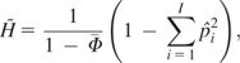
Consider a polymorphic locus with I distinct alleles and a population with parametric allele frequencies p₁, p₂, … ,p_I, where p_i ∈ [0, 1] and ∑_{i = 1}^Ip_i = 1. The term “gene diversity,” which is defined as

(1)

was proposed by Nei (1973), though the use of equation (1) as a measure of diversity dates to considerably earlier (Gini 1912; Simpson 1949; Gibbs and Martin 1962).

Now consider a sample of n observations of alleles, in which the number of observations of allelic type i is n_i. The count estimate of p_i is ${\widehat{p}}_i=n_i/n$. If no inbred or related individuals are included in the sample, then an unbiased estimator of gene diversity is (Nei and Roychoudhury 1974)

(2)

If relatives or inbred individuals are included in the sample, then $\widehat{H}$ is no longer an unbiased estimator of H. To understand why this statement is true, suppose that a sample contains a pair of close relatives. Because these individuals are related, they may share one or two alleles identically by descent (IBD) at a locus (compared with zero alleles shared IBD in unrelated individuals). As a result, estimation of p_i is based on fewer independent observations than for a sample not containing any relatives. Although $E\left[{\widehat{p}}_i\right]=p_i$ when relatives are included, $\text{Var}\left[{\widehat{p}}_i\right]$ is greater than it would be had no relatives been included. Observe that the computation of $E\left[\widehat{H}\right]$ involves a negative coefficient for $E\left[{\widehat{p}}_i^2\right]$. Because $E\left[{\widehat{p}}_i^2\right]=\text{Var}\left[{\widehat{p}}_i\right]+E{\left[{\widehat{p}}_i\right]}^2$, $E\left[\widehat{H}\right]$ decreases as $\text{Var}\left[{\widehat{p}}_i\right]$ increases. Thus, the inclusion of relatives results in a downward bias, so that $E\left[\widehat{H}\right]<H$. For the case in which inbred unrelated individuals with known inbreeding coefficients are included in a sample, Weir (1989, 1996) provided the expectation of $1-{\displaystyle {\sum }_{i=1}^I{\widehat{p}}_i^2}$, producing an unbiased estimator of gene diversity

(3)

where is the average inbreeding coefficient across individuals (see also Shete 2003). When inbred individuals are included, ≠0, and it follows that $E\left[\widehat{H}\right]<E\left[{\widehat{H}}_{\text{Weir}}\right]=H.$

In this article, we conduct a detailed investigation of the case in which a sample includes related individuals. We derive an unbiased estimator of H for samples containing related individuals with known levels of relationship. Our derivation makes use of a formula of Bourgain et al. (2003) and McPeek et al. (2004) for the variance of count estimates of allele frequencies in samples containing inbred and related individuals. The resulting estimator incorporates kinship coefficients, the same quantitative descriptors of pairwise relationships that have been used in diverse problems involving relatives—such as evaluation of phenotypic covariances in families (Lange 2002), estimation of relatedness parameters (Weir et al. 2006), and quantitative-trait linkage analysis (Almasy and Blangero 1998). When a sample consists only of unrelated noninbred individuals, our new estimator $\tilde{H}$ reduces to the standard estimator $\widehat{H}$, and it reduces to ${\widehat{H}}_{\text{Weir}}$ if inbred but not related individuals are included. Using data simulated based on allele frequencies from human populations, we find that the new estimator $\tilde{H}$ corrects for bias generated by inclusion of related individuals and that it attains a mean squared error (MSE) comparable with that of $\widehat{H}$. We apply this new estimator to microsatellite data from human population samples containing relatives and show that, compared with the standard estimator, it produces estimates closer to those obtained when excluding relatives from the analysis.

Theory

We assume that gene diversity is estimated from n/2 diploid individuals. Our aim is to obtain a bias-correction factor that can be incorporated into a new estimator of gene diversity, $\tilde{H}.$ We begin by computing $\text{Var}\left[{\widehat{p}}_i\right]$ in a sample that may include relatives or inbred individuals. $\text{Var}\left[{\widehat{p}}_i\right]$ was reported by Bourgain et al. (2003) and McPeek et al. (2004); we provide an alternative derivation that uses a generalization of the simpler method of Broman (2001). This approach was originally applied in a setting that did not consider inbreeding, and we generalize the computation to include inbreeding. Note that the variances of other estimators of allele frequencies have previously been derived in fairly general settings (McPeek et al. 2004) and that the estimator ${\widehat{p}}_i$ is not a maximum likelihood estimator when related individuals are included in a sample (Boehnke 1991). However, our interest here is specifically on the count-based estimator of allele frequencies, as it is this estimator that is used in the standard estimator of gene diversity in equation (2).

Define X_k to be the number of alleles of type i that are carried by individual k at a particular locus. X_k can equal 0, 1, or 2, and E[X_k] = 2p_i. Regardless of the relationships among individuals 1, 2, …, n/2, an unbiased estimator for p_i, the frequency of allele i, is

(4)

The variance of ${\widehat{p}}_i$ is given by

(5)

Suppose that individuals j and k are related. The coefficient of kinship between individuals j and k, Φ_j,k, is the probability that two alleles chosen at the locus—one from individual j and the other from individual k—are identical by descent. In the special case of j = k, the kinship coefficient is Φ_k,k = (1/2)(1 + f_k), where f_k is the inbreeding coefficient for individual k (Lange 2002, p. 81).

Conditional on the nature of the relationship between individuals j and k and on their inbreeding coefficients, the four alleles in the two individuals can take on one of nine condensed identity states (Jacquard 1974, p. 107). Let Δ_s = Pr[S = s], where the condensed identity state S ranges from 1 to 9 and the probability is conditional on the type of the relationship. Using table 1 and the fact that the kinship coefficient for the pair of individuals equals Δ₁ + (1/2)(Δ₃ + Δ₅ + Δ₇) + (1/4)Δ₈ (Jacquard, 1974, p. 108), we obtain

Because E[X_j] = E[X_k] = 2p_i, it follows that

(6)

Inserting the covariance into equation (5) yields

(7)

where 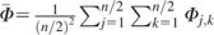is the average kinship coefficient across pairs of individuals (including comparisons of individuals with themselves). This result can be seen to be equivalent to the variance reported by McPeek et al. (2004, p. 361).

Proposition 1

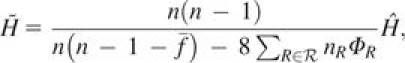
Consider a locus with I distinct alleles, allele frequencies p_i ∈ [0, 1] and ${\displaystyle {\sum }_{i=1}^I{p}_i}=1$. Suppose a sample from a population has n/2 possibly related and inbred individuals. Then an unbiased estimator for gene diversity is

(8)

where Φ_j,k is the kinship coefficient of individuals j and k and is the average kinship coefficient across pairs of individuals.

Proof

We need to show that $E\left[\tilde{H}\right]=H$. Observing that $E\left[{\widehat{p}}_i^2\right]=\text{Var}\left[{\widehat{p}}_i\right]+E{\left[{\widehat{p}}_i\right]}^2$ and $E\left[{\widehat{p}}_i\right]=p_i$, we apply equation (4) and then the variance of ${\widehat{p}}_i$ in equation (7) to get

Corollary 2

Consider a locus with I distinct alleles, allele frequencies p_i ∈ [0, 1] and ${\displaystyle {\sum }_{i=1}^I{p}_i}=1$. Suppose a sample from a population has n/2 possibly related and inbred individuals. Let ℛ be the set of distinct types of relative pairs in the sample. Further, let n_R be the number of pairs of individuals with relationship type $R\in \mathcal{ℛ}$ and let Φ_R be the kinship coefficient for each of these pairs. Then an unbiased estimator for gene diversity is

(9)

where is the average inbreeding coefficient across individuals and f_k is the inbreeding coefficient for individual k.

Proof

Applying the definitions of and Φ_k,k and the fact that Φ_j,k = 0 for a pair of “unrelated” individuals,

Inserting this value for into equation (8), we obtain the desired result.□

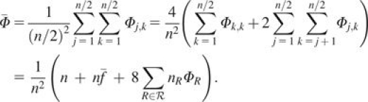
Table 1.

Joint Distribution of the Numbers of i Alleles Carried by Individuals j and k Given Their Descent Configuration S, Assuming Allele i Has Frequency p

Note that if no related individuals are included in the sample, then ℛ is the empty set, thus reducing $\tilde{H}$ to ${\widehat{H}}_{\text{Weir}}$; if additionally no inbred individuals are included, then =0 and $\tilde{H}$ reduces to $\widehat{H}$.

Corollary 3

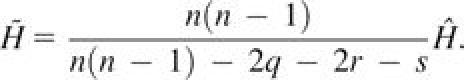
Consider a locus with I distinct alleles, allele frequencies p_i ∈ [0, 1] and ${\displaystyle {\sum }_{i=1}^I{p}_i}=1$. Suppose a sample from a population has n/2 noninbred individuals, among which q parent–offspring pairs, r full-sib pairs, and s second-degree (avuncular, grandparent–grandchild, and half-sib) relative pairs are included. Assuming the sample has no other relative pairs, an unbiased estimator for gene diversity is

(10)

Proof

The kinship coefficients are Φ_P = 1/4 for parent–offspring pairs, Φ_F = 1/4 for full-sib pairs, and Φ_S = 1/8 for second-degree pairs. If an individual k is not inbred, then f_k = 0. For a sample without inbred individuals, =0. Inserting the quantity and kinship coefficient for each of the three types of relative pairs into equation (9), we obtain equation (10).□

Corollary 4

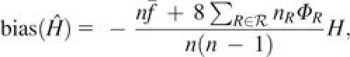
Consider a locus with I distinct alleles, allele frequencies p_i ∈ [0, 1] and ${\displaystyle {\sum }_{i=1}^I{p}_i}=1$. Suppose a sample from a population has n/2 possibly related and inbred individuals. Let ℛ be the set of distinct types of relative pairs in the sample. Further, let n_R be the number of pairs of individuals with relationship type R∈ℛ and let Φ_R be the kinship coefficient for each of these pairs. Then the bias of $\widehat{H}$ is always negative, increases in magnitude as H increases, and is given by

(11)

where is the average inbreeding coefficient across individuals and f_k is the inbreeding coefficient for individual k.

Proof

As shown in Corollary 2, $\tilde{H}=c\widehat{H}$, where c=n(n−1)/[n(n−1−)−8∑_R∈ℛn_RΦ_R]. Rearranging and taking the expected value gives $E\left[\widehat{H}\right]=E\left[\tilde{H}\right]/c=H/c$. The desired result follows from simplifying the expression for $\text{bias}\left(\widehat{H}\right)$, or (1 − c)H/c.□

Data from Human Populations

To examine the behavior of $\tilde{H}$ in a realistic setting, we performed simulations and data analysis using microsatellite loci from the H1048 and H952 subsets (Rosenberg 2006) of the Human Genome Diversity Project–Centre d'Etude du Polymorphisme Humain (HGDP–CEPH) Cell Line Panel (Cann et al. 2002; Cavalli-Sforza 2005). The H1048 subset consists of 1,048 individuals in 53 populations. Among the 53 populations, the samples from 26 of them contain at least one pair of closely related individuals with either a first-degree (parent–offspring, full-sib) or second-degree (avuncular, grandparent–grandchild, and half-sib) relationship (table 2). The H952 subset is a collection of 952 individuals included in the larger H1048 subset. No two of the 952 individuals are believed to have a first- or second-degree relationship. Levels of relationship in H1048, as estimated previously from microsatellite genotypes (Rosenberg 2006), were treated here as known with certainty. Because no cycles were observed in pedigrees from the HGDP–CEPH panel (Rosenberg 2006), we assumed that none of the panel members were inbred. Genotypes at 783 autosomal microsatellite loci (Ramachandran et al. 2005; Rosenberg et al. 2005) were investigated in the H1048 and H952 data sets.

Table 2.

The 26 Populations Containing Relatives in the H1048 Data Set (Modified from Rosenberg 2006, Supplementary tables 16 and 19)

Population	Geographic Region	Number of Sampled Individuals	Number of Parent–Offspring Pairs	Number of Full-Sib Pairs	Number of Second-Degree Pairs
Bantu (Kenya)	Africa	12	0	1	0
Biaka Pygmy	Africa	32	4	2	7
Mandenka	Africa	24	0	0	2
Mbuti Pygmy	Africa	15	2	0	1
San	Africa	7	1	0	0
Yoruba	Africa	25	2	2	0
French	Europe	29	0	1	0
Orcadian	Europe	16	1	0	0
Bedouin	Middle East	48	1	0	1
Druze	Middle East	47	1	2	2
Mozabite	Middle East	30	0	1	0
Palestinian	Middle East	51	0	1	5
Balochi	Central/South Asia	25	0	1	0
Hazara	Central/South Asia	24	0	1	1
Kalash	Central/South Asia	25	1	0	1
Sindhi	Central/South Asia	25	1	0	0
Cambodian	East Asia	11	1	0	0
Lahu	East Asia	10	1	1	0
Naxi	East Asia	10	0	1	0
Oroqen	East Asia	10	0	1	0
Melanesian	Oceania	19	9	3	2
Colombian	America	13	6	1	0
Karitiana	America	24	6	6	0
Maya	America	25	2	1	2
Pima	America	25	15	6	10
Surui	America	21	15	14	0

Simulations

Simulation Procedure

Simulations based on the microsatellite loci were used to examine the properties of $\tilde{H}$ and $\widehat{H}$. For each of the 783 loci, we treated allele frequencies estimated from the H952 subset of individuals as true allele frequencies. The parametric gene diversity H was obtained for a locus as one minus the sum of the squares of these allele frequencies. All of our simulations assumed no inbreeding.

For a given locus, individual genotypes were simulated by sampling two alleles independently from the allele frequency distribution. To simulate a related individual with a given level of relationship to another individual, the number of alleles shared IBD with its relative was drawn under the appropriate probability distribution for the specified type of relative pair (parent–offspring, full-sib, or second-degree). This number of shared alleles (0, 1, or 2) was copied from a random individual that had already been generated and that had not yet been paired with a relative; if the number of alleles copied was 1, then an allele was chosen at random from the previously generated individual. The rest of the alleles, if any, were sampled independently from the allele frequency distribution. Gene diversity was estimated using $\tilde{H}$ and $\widehat{H}$ for samples with and without related individuals. We applied $\widehat{H}$ both to entire samples as well to samples in which the “second” member of each relative pair was discarded. For each locus, simulated sets of individuals were obtained 100,000 times, and $\widehat{H}$, $\tilde{H}$, ${\widehat{H}}^2$, and ${\tilde{H}}^2$ were averaged across all replicates. The true value for gene diversity, H, was then subtracted from the mean of $\widehat{H}$ and $\tilde{H}$ to calculate bias for each estimator (and the result was squared to give bias squared). Variance of $\widehat{H}$ was calculated by subtracting the square of the mean of $\tilde{H}$ from the mean of ${\widehat{H}}^2$ (variance of $\tilde{H}$ was calculated analogously). MSE was then calculated by adding variance and bias squared. Note that in our simulations, relative pairs were all disjoint, so that no individual was contained in multiple relative pairs; however, in our derivations, it is not required for relative pairs to be disjoint for $\tilde{H}$ to be unbiased.

Simulation Results

To illustrate the performance of the estimators across the span of gene diversities present in the human microsatellite data set, loci were placed in increasing order by assumed parametric gene diversity, and six equally spaced loci—with the 112th, 224th, 336th, 448th, 560th, and 672nd highest values of gene diversity—were chosen for analysis. Similar results were obtained with all six loci (data not shown), and therefore, among the six loci only the locus with the lowest gene diversity (AAT263P, H = 0.6778) and the locus with the highest gene diversity (ACT3F12, H = 0.8263) were chosen for display. For both loci, table 3 shows the simulated MSE, variance, and bias squared for the different estimators, considering three different sample sizes and three combinations of the number of related individuals for each sample size. Because the simulation results are based on 100,000 replicate data sets, each of the quantities presented is small. However, it is possible to observe differences in the properties of the three estimators. Among the three estimators, $\widehat{H}$ applied to full samples gives the lowest variance, $\tilde{H}$ produces slightly higher variance, and $\widehat{H}$ applied to samples with related individuals removed produces the highest variance. Bias squared is very close to zero for $\widehat{H}$ applied to samples with related individuals removed, as well as for $\tilde{H}$, but it is noticeably higher for $\widehat{H}$ applied to full samples containing relatives. For the locus with the lower value of H (0.6778), $\widehat{H}$ applied to full samples has the smallest MSE in all cases tested, although $\tilde{H}$ has MSE very close to that of $\widehat{H}$. However, for the locus with the higher value of H (0.8263), MSE is always smallest for $\tilde{H}$. Therefore, $\tilde{H}$ is not only unbiased, but it also has MSE comparable with—and sometimes smaller than—that of $\widehat{H}$.

Table 3.

MSE, Variance, and Bias Squared of Estimates for Data Simulated Based on Allele Frequencies at Two Loci (AAT263P and ACT3F12)

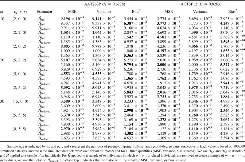It is instructive to investigate the influence of specific variables on the MSE, variance, and bias squared of $\tilde{H}$ and $\widehat{H}$, by varying the simulation parameters over the space of gene diversities, sample sizes, and possible sets of relative pairs, and calculating MSE, variance, and bias squared for each scenario. We use ${\widehat{H}}_{\text{full}}$ and ${\tilde{H}}_{\text{full}}$ to denote $\widehat{H}$ and $\tilde{H}$ applied to a sample of individuals. For $\widehat{H}$ applied to a sample in which related individuals are removed, we use the notation ${\widehat{H}}_{\text{reduced}}$.

Figure 1 displays the effect of sample size on MSE for each of the estimators, for scenarios in which all simulated individuals belong to relative pairs of a particular type. Here, the full and reduced samples consist of m and m/2 individuals, respectively. When q = m/2, r = m/2, or s = m/2, MSE is consistently lower for ${\widehat{H}}_{\text{full}}$ and ${\tilde{H}}_{\text{full}}$ (which have virtually identical MSE and therefore have overlapping lines in the graph) than for ${\widehat{H}}_{\text{reduced}}$. As the sample size increases, the MSEs of all estimators approach zero.

FIG. 1.—

MSE as a function of sample size m for three different estimators. Each plot in a given row represents samples with a different type of relative pair. The numbers of parent–offspring, full-sib, and second-degree pairs are denoted by q, r, and s, respectively. The full and reduced samples contain m and m/2 individuals, respectively. The ${\tilde{H}}_{\text{full}}$ curve is almost directly on top of the ${\widehat{H}}_{\text{full}}$ curve. (A) Allele frequencies simulated based on observed frequencies at locus AAT263P (H = 0.6778). (B) Allele frequencies simulated based on observed frequencies at locus ACT3F12 (H = 0.8263). The range of the plots is truncated at 0.02, so that the MSE for small sample sizes is not shown. Each point in the graphs is based on 100,000 simulated data sets, and the same simulated data were used for all three estimators.

We next examined how the three estimators performed in simulated samples containing the same sample size and total number of relative pairs but with different combinations involving different numbers of parent–offspring, full-sib, and second-degree pairs. The same two loci that were analyzed in table 3 and figure 1 were investigated to show the effect of the combination of relative pairs at differing degrees of gene diversity. Figures 2 and 3 illustrate MSE, variance, and bias squared for each estimator as functions of the combination of types of relative pairs in a full sample of size 40 and a reduced sample of size 20 individuals. Each point in a triangle represents the number of parent–offspring, full-sib, and second-degree relative pairs in a sample; the sum of these quantities is equal to half the sample size. MSE and variance are always lower for ${\widehat{H}}_{\text{full}}$ and ${\tilde{H}}_{\text{full}}$ than for ${\widehat{H}}_{\text{reduced}}$, which relies on a smaller sample size, and ${\widehat{H}}_{\text{full}}$ and ${\tilde{H}}_{\text{full}}$ show similar trends. Bias squared for the unbiased ${\tilde{H}}_{\text{full}}$ is similar to that for ${\widehat{H}}_{\text{reduced}}$, which eliminates relatives from the sample, whereas it is much larger for ${\widehat{H}}_{\text{full}}$. As the number of first-degree pairs is increased (decreasing the number of second-degree pairs), both variance and MSE increase. For ${\widehat{H}}_{\text{full}}$, as can be predicted from equation (11), bias squared also increases with an increase in the number of first-degree pairs. Because they are both unbiased estimators, ${\widehat{H}}_{\text{full}}$ and ${\widehat{H}}_{\text{reduced}}$ display no particular pattern for bias squared.

FIG. 2.—

Heat maps of simulated MSE, variance, and bias squared for each estimator applied to a full sample of 40 and a reduced sample of 20 individuals, as functions of the mixture of types of relative pairs included in the sample. The simulation was based on allele frequencies at the AAT263P locus (H = 0.6778). The sample of 40 individuals includes q parent–offspring, r full-sib, and s second-degree pairs. The three vertices correspond to samples that contain either all parent–offspring, all full-sib, or all second-degree pairs. Moving horizontally along the triangle changes the numbers of parent–offspring and full-sib pairs in the sample and moving vertically changes the number of second-degree pairs. The numbers indicated on the scale are the cutoff values for each color. Each row of triangles represents a different estimator, and each column represents a different statistic. Blue and black dots represent the points at which the smallest and largest values occur in each triangle, respectively. Each point in the graphs is based on 100,000 simulated data sets, and the same simulations were used for all three estimators.

FIG. 3.—

Heat maps of simulated MSE, variance, and bias squared for each estimator applied to a full sample of 40 and a reduced sample of 20 individuals, as functions of the mixture of types of relative pairs included in the sample. The simulation was based on allele frequencies at the ACT3F12 locus (H = 0.8263). See figure 2 caption for additional details.

Finally, we studied the trends in MSE, variance, and bias squared for the estimators over the space of gene diversities, holding the full sample size fixed at 30 individuals and the reduced sample size fixed at 15. Unlike the analyses in table 3 and figures 1–3, which show results based on two representative loci, this analysis used simulations based on all 783 microsatellites. We considered a scenario in which the sample of 30 individuals consisted of 15 parent–offspring pairs. Figure 4 illustrates that for all three estimators, MSE and variance tend to decrease as gene diversity increases. Because ${\tilde{H}}_{\text{full}}$ and ${\widehat{H}}_{\text{reduced}}$ are both unbiased, bias squared shows no trend for these estimators. However, because bias for ${\widehat{H}}_{\text{full}}$ is linear with respect to gene diversity (eq. 11), bias squared is quadratic. On the basis of equation (11), we predict , and a close match to this prediction was observed. The regression displayed in figure 4 has regression model ${\left[\text{bias}\right({\widehat{H}}_{\text{full}}\left)\right]}^2=(7.187\times {10}^{-5})H^2$.

FIG. 4.—

MSE, variance, and bias squared for each estimator applied to a full sample of 30 and a reduced sample of 15 individuals, as functions of parametric gene diversity, considering simulated values based on each of the 783 loci. The simulations incorporated 30 individuals in 15 parent–offspring pairs. (A) ${\widehat{H}}_{\text{full}}$. A quadratic regression of bias squared on H (with the constant and linear terms forced to be 0) is given by (7.187 × 10⁻⁵)H², with R² = 0.959. The Spearman correlation coefficient is −0.8364 for H and MSE and −0.8394 for H and variance. (B) ${\tilde{H}}_{\text{full}}$. The Spearman correlation coefficient is −0.8394 for H and MSE and −0.8394 for H and variance. (C) ${\widehat{H}}_{\text{reduced}}$. The Spearman correlation coefficient is −0.8447 for H and MSE and −0.8447 for H and variance. Each point in the graphs is based on 100,000 simulated data sets, and the same simulations were used for all three estimators.

Three main results can be observed in our simulations. First, $\tilde{H}$ is unbiased and has comparable bias in samples containing relatives to that obtained by applying $\widehat{H}$ to samples with relatives removed. Using $\tilde{H}$, or excluding relatives and using $\widehat{H}$, reduces the bias compared with using $\widehat{H}$ without excluding relatives. Second, $\widehat{H}$ has comparable (but consistently slightly higher) variance to the values obtained with $\widehat{H}$ in samples containing relatives. Both $\tilde{H}$ and $\widehat{H}$ have lower variance in full samples of individuals than that of $\widehat{H}$ in reduced samples that exclude relatives. Third, because $\tilde{H}$ has less bias than $\widehat{H}$ in samples containing relatives, $\tilde{H}$ has comparable, and sometimes smaller, MSE to $\widehat{H}$ (although its variance is larger). Both estimators have lower MSE than $\widehat{H}$ applied to subsets that exclude relatives.

The properties of the estimators depend on a number of parameters. All estimators have lower MSE as sample size increases. In addition, the MSEs of $\widehat{H}$ and $\tilde{H}$ are smaller when second-degree relative pairs are investigated, in comparison to scenarios that include an equivalent number of first-degree pairs. Furthermore, the MSEs of $\widehat{H}$ and $\tilde{H}$ are generally smaller for loci with larger gene diversities, with the magnitude of the bias of $\widehat{H}$ increasing linearly with increasing gene diversity.

We can conclude that for samples containing relatives, $\tilde{H}$ has comparable variance to $\widehat{H}$, with a considerable reduction of bias. $\tilde{H}$ has comparable bias in a full sample to that of $\widehat{H}$ applied to a reduced sample excluding relatives, with a considerable reduction of variance. Thus, $\tilde{H}$ combines into a single estimator the desirable properties possessed by $\widehat{H}$ applied to samples with relatives and by $\widehat{H}$ applied to samples without relatives.

Application to Data

Notation

For convenience, we use the following notation: ${\widehat{H}}_{952}$ and ${\widehat{H}}_{1048}$ for application of $\widehat{H}$ to the samples of 952 and 1,048 individuals, respectively, and ${\tilde{H}}_{952}$ and ${\tilde{H}}_{1048}$ for application of $\tilde{H}$ to these samples. Note that because the H952 data set contains no relative pairs, ${\tilde{H}}_{952}={\widehat{H}}_{952}$, and there is no need to consider ${\tilde{H}}_{952}$ separately. We also use the notation ${\widehat{H}}_{507}$, ${\widehat{H}}_{603}$, and ${\tilde{H}}_{603}$ when restricting our analysis to the 26 populations containing at least one relative pair; for each of the 27 remaining populations, the estimators $\widehat{H}$ and $\tilde{H}$ produce identical values.

Mean of the Estimator

For investigating the properties of $\widehat{H}$ and $\tilde{H}$ applied to the H1048 data set, because the true value of H is unknown for the actual data, we treated the value of ${\widehat{H}}_{952}$ for each locus as a substitute “true” value. Because $\widehat{H}$ is unbiased when applied to data not containing relatives, ${\widehat{H}}_{952}$ provides a sensible proxy for the unknown true gene diversity. This approach enabled us to consider how estimates of H from data including relatives might differ from estimates based on the same data excluding all relatives. For each of the 53 populations, we computed the means of ${\widehat{H}}_{952}$, ${\widehat{H}}_{1048}$, and ${\tilde{H}}_{1048}$ across the 783 microsatellite loci. Because the true H is unknown and bias cannot be calculated, we instead examine the mean of ${\widehat{H}}_{1048}$ across loci minus the mean of ${\widehat{H}}_{952}$ across loci and the mean of ${\tilde{H}}_{1048}$ across loci minus the mean of ${\widehat{H}}_{952}$ across loci.

Figure 5 shows comparisons of the mean of ${\widehat{H}}_{1048}-{\widehat{H}}_{952}$ across loci and the mean of ${\tilde{H}}_{1048}-{\widehat{H}}_{952}$ across loci. In general, the three estimators produce similar estimates in a given population. However, notice that in figure 5A, ${\widehat{H}}_{1048}$ is reduced compared with ${\widehat{H}}_{952}$, a likely consequence of the bias of $\widehat{H}$ when applied to samples containing relatives. When ${\tilde{H}}_{1048}$ is used in place of ${\widehat{H}}_{1048}$, because ${\tilde{H}}_{1048}$ corrects for the inclusion of known related individuals, there is a considerable reduction in the magnitude of the difference between the mean of the estimator (${\widehat{H}}_{1048}$ or ${\tilde{H}}_{1048}$) across loci and the mean of ${\widehat{H}}_{952}$ across loci (fig. 5B). These observations are reflected in Wilcoxon signed rank tests that compare paired lists of mean heterozygosities across loci for the 53 populations (table 4). The P value for a comparison of ${\widehat{H}}_{1048}$ with ${\widehat{H}}_{952}$ was 8.804 × 10⁻⁶, suggesting that inclusion of relatives in a sample has a statistically significant impact on $\widehat{H}$. In contrast, ${\tilde{H}}_{1048}$ and ${\widehat{H}}_{952}$ showed no significant difference, with a P value of 0.703 for the Wilcoxon signed rank test. Similar results were obtained for other comparisons of the three estimators. The mean across populations of ${\widehat{H}}_{952}-{\tilde{H}}_{1048}(3.262\times {10}^{-4})$ was smaller than for ${\widehat{H}}_{952}-{\widehat{H}}_{1048}(2.387\times {10}^{-3})$; the same was true for the mean of $|{\widehat{H}}_{952}-{\tilde{H}}_{1048}|(6.660\times {10}^{-4})$ compared with the mean of $|{\widehat{H}}_{952}-{\widehat{H}}_{1048}|(2.387\times {10}^{-3})$.

FIG. 5.—

Comparison of the mean of ${\widehat{H}}_{1048}-{\widehat{H}}_{952}$ and the mean of ${\tilde{H}}_{1048}-{\widehat{H}}_{952}$. Each population is represented by a point colored based on the geographic location of the population, and the dotted line represents zero difference between the full-data estimator and ${\widehat{H}}_{952}$. Because 27 of the 53 populations do not contain related individuals, the gene diversities given by ${\widehat{H}}_{1048}$ and ${\tilde{H}}_{1048}$ are the same for these populations. (A) The mean of ${\widehat{H}}_{1048}-{\widehat{H}}_{952}$, displaying a reduction of $\widehat{H}$ when applied to samples containing related individuals. (B) The mean of ${\widehat{H}}_{1048}-{\widehat{H}}_{952}$, displaying a decrease in the magnitude of the difference between the full-data estimator and ${\widehat{H}}_{952}$.

Table 4.

Statistical Tests Applied to the Mean Gene Diversity across Loci

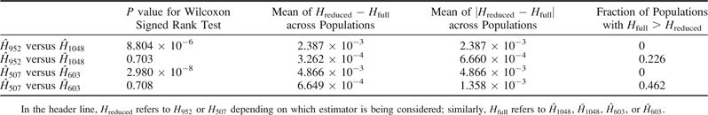Comparable results were obtained when using only the 26 populations that contained relative pairs. The Wilcoxon signed rank test produced a statistically significant P value of 2.980 × 10⁻⁸ for ${\widehat{H}}_{603}$ compared with ${\widehat{H}}_{507}$ and a nonsignificant P value of 0.708 when comparing ${\tilde{H}}_{603}$ with ${\widehat{H}}_{507}$. The mean across populations of ${\widehat{H}}_{507}-{\tilde{H}}_{603}(6.649\times {10}^{-4})$ was smaller than for ${\widehat{H}}_{507}-{\widehat{H}}_{603}(4.866\times {10}^{-3})$, as was the mean of $|{\widehat{H}}_{507}-{\tilde{H}}_{603}|(1.358\times {10}^{-3})$ relative to that of $|{\widehat{H}}_{507}-{\widehat{H}}_{603}|(4.866\times {10}^{-3})$. In addition, similar numbers of populations had ${\tilde{H}}_{603}>{\widehat{H}}_{507}\text{(12)}$ and ${\tilde{H}}_{603}<{\widehat{H}}_{507}\text{(14)}$; by contrast, there were no populations with ${\widehat{H}}_{603}>{\widehat{H}}_{507}$.

Because estimators often have a trade-off between bias and variance, we investigated the relationship between the mean values across loci of ${\widehat{H}}_{603}-{\widehat{H}}_{507}$ and ${\tilde{H}}_{603}-{\widehat{H}}_{507}$ and the standard deviations of ${\widehat{H}}_{603}$ and ${\tilde{H}}_{603}$ across loci. We observed that compared with ${\widehat{H}}_{603}$, ${\tilde{H}}_{603}$ produces a noticeable decrease in the mean difference from ${\widehat{H}}_{507}$ with only a slight increase in the standard deviation (fig. 6). This result is somewhat analogous to the simulation-based result that $\tilde{H}$ has less bias than $\widehat{H}$ and comparable variance.

FIG. 6.—

Comparison of the mean difference of an estimator (${\widehat{H}}_{603}$ or ${\tilde{H}}_{603}$) from ${\widehat{H}}_{507}$ with the standard deviation of the estimator. Each population is represented by a point colored based on the geographic location of the population. Open and filled circles represent the estimates for ${\widehat{H}}_{603}$ and ${\tilde{H}}_{603}$, respectively.

Gene Diversity versus Distance from Africa

Based on an observed decline of gene diversity estimates with geographic distance from East Africa, Ramachandran et al. (2005) argued that the geographic expansion of modern humans can be described by a series of founder events originating in Africa. This analysis utilized the $\widehat{H}$ estimator applied to the 783 microsatellites typed in the H1048 subset of individuals, excluding the Surui population. To evaluate how the results of Ramachandran et al. (2005) were affected by the bias of $\widehat{H}$ in samples with close relatives, we analyzed the relationships of the three estimators of gene diversity—${\widehat{H}}_{952}$, ${\widehat{H}}_{1048}$, and ${\tilde{H}}_{1048}$—with geographic distance from East Africa (fig. 7). Distance from Addis Ababa was measured in kilometers via waypoint routes and was based on the values from Rosenberg et al. (2005).

FIG. 7.—

Gene diversity versus geographic distance from Addis Ababa, Ethiopia. (A) ${\widehat{H}}_{952}$ versus distance from Addis Ababa. The linear regression is given by H = 0.7778 − (7.955 × 10⁻⁶) × distance, with R² = 0.856. (B) ${\widehat{H}}_{1048}$ versus distance from Addis Ababa. The linear regression is given by H = 0.7809 − (8.595 × 10⁻⁶) × distance, with R² = 0.844. (C) ${\tilde{H}}_{1048}$ versus distance from Addis Ababa. The linear regression is given by H = 0.7792 − (8.161 × 10⁻⁶) × distance, with R² = 0.849.

The three estimators produced relatively similar regressions (fig. 7), demonstrating that the close linear relationship of gene diversity and distance from Africa is not greatly affected by inclusion of relatives in the analysis. We observed very similar values for the coefficients of determination (R²) of linear regressions when using ${\widehat{H}}_{952}$, ${\widehat{H}}_{1048}$, and ${\tilde{H}}_{1048}$ (note that all three R² values are higher than that reported by Ramachandran et al. (2005), whose lower value resulted from an error in the calculation of their fig. 4A). The Surui population, which has the smallest gene diversity and is the farthest population from Addis Ababa, deviates considerably from the regression line when using ${\widehat{H}}_{1048}$ to measure gene diversity (fig. 7B). When excluding the large number of relatives present in the Surui sample (${\widehat{H}}_{952}$) or correcting for their inclusion (${\tilde{H}}_{1048}$), the Surui population is not as extreme an outlier (fig. 7A and C).

Discussion

In this article, we have developed an unbiased estimator $\tilde{H}$ for gene diversity in samples containing related and inbred individuals. The bias-correction factor in this estimator, which we derived from the variance of allele frequency estimates, depends only on the average kinship coefficient between pairs of sampled individuals. Using data simulated based on allele frequency distributions from human populations, we found that $\tilde{H}$ performs well with regard to both bias and MSE. The bias generated by $\tilde{H}$ applied to data including relatives is approximately the same as the bias generated by the standard estimator $\widehat{H}$ applied to data containing only unrelated individuals. The MSE for $\tilde{H}$ is comparable to—and often smaller than—the MSE of $\widehat{H}$ when related individuals are included. Calculation of $\tilde{H}$ relies only on sample allele frequencies and on the average kinship coefficient and is therefore easy to perform when relationships among individuals are known. Thus, the new estimator $\tilde{H}$ offers a combination of unbiasedness, low MSE, and ease of computation, providing an improved approach to the estimation of gene diversity in samples containing relatives.

Using data from human populations, we found that $\tilde{H}$ largely corrected a reduction in the standard estimator $\widehat{H}$, producing estimates that were not significantly different from those obtained if we instead removed relatives from the data set and applied $\widehat{H}$. This shift toward the values obtained in data without relatives occurred together with only a slight increase in standard deviation across loci relative to $\widehat{H}$. However, by treating dependent observations as independent, $\widehat{H}$ perhaps produces a smaller variance than is appropriate in samples with relatives. Thus, we conclude that as an alternative to removing relatives from samples containing relative pairs, $\tilde{H}$ can be applied to obtain suitable gene diversity estimates.

When we applied $\tilde{H}$ to the human data, a few populations still produced a “bias,” in that ${\tilde{H}}_{1048}$ remained considerably lower than ${\widehat{H}}_{952}$. The most noticeable of these populations are the Surui, Karitiana, and Pima populations from the Americas (fig. 5B); the “bias” was larger for these low-diversity populations, whereas theory predicts less bias when diversity is lower (eq. 11). It should first be noted that unlike for the other populations, inferences about second-degree relationships obtained by Rosenberg (2006) were somewhat uncertain for the Surui and Karitiana populations. Thus, table 2 and our analysis did not include inferred second-degree relationships in those populations, when in fact many are likely to be present. This is a likely reason why the “bias” in the Surui and Karitiana populations was only partially eliminated. For the Pima population, a likely explanation is that the sample contains many related individuals in extended families (Rosenberg, 2006), and our computation only adjusted for first- and second-degree relative pairs. If these higher order relationships had been fully known, however, it would have been possible to use our estimator to adjust for them.

Our estimator adjusts for inbreeding by averaging over inbreeding coefficients for sampled individuals. It is important to note that the inbreeding coefficients that we have included are exact values obtained from pedigrees. If an estimated inbreeding coefficient was used in place of the exact value, then $\tilde{H}$ would not necessarily produce unbiased estimates in samples containing inbred individuals. $\tilde{H}$ would also lead to a bias if relationships were misspecified. In our data example, relationships were assumed to be known, and for a data set of the size used for inferring the relationships (Rosenberg 2006) this assumption is generally sensible. However, for small data sets in which relationship inferences are uncertain, caution must be used when interpreting the bias of $\tilde{H}$ applied to the same data from which relationships are estimated.

The estimators we have considered relate to within-population gene diversity. What if we consider the gene diversity between populations? Suppose we have samples from two populations, A and B, each containing related inbred individuals. The between-population analog of gene diversity is ${\widehat{H}}_{A,B}=1-{\displaystyle {\sum }_{i=1}^I{\widehat{p}}_i{\widehat{q}}_i}$, where ${\widehat{p}}_i$ and ${\widehat{q}}_i$ are estimates of the frequency of allele i at a given locus in populations A and B, respectively (Nei 1987). Because the bias in within-population gene diversity estimates only arises from the quadratic ${\widehat{p}}_i^2$ term in equation (1), $E\left[{\displaystyle {\sum }_{i=1}^I{\widehat{p}}_i}{\widehat{q}}_i\right]={\displaystyle {\sum }_{i=1}^I{p}_i}{q}_i$ (Nei 1987, p. 222), and ${\widehat{H}}_{A,B}$ continues to be an unbiased estimator for between-population gene diversity in samples containing relatives.

References

- Almasy L, Blangero J. Multipoint quantitative-trait linkage analysis in general pedigrees. Am J Hum Genet. 1998;62:1198–1211. doi: 10.1086/301844. [DOI] [PMC free article] [PubMed] [Google Scholar]
- Boehnke M. Allele frequency estimation from data on relatives. Am J Hum Genet. 1991;48:22–25. [PMC free article] [PubMed] [Google Scholar]
- Bourgain C, Hoffjan S, Nicolae R, Newman D, Steiner L, Walker K, Reynolds R, Ober C, McPeek MS. Novel case–control test in a founder population identifies P-selectin as an atopy-susceptibility locus. Am J Hum Genet. 2003;73:612–626. doi: 10.1086/378208. [DOI] [PMC free article] [PubMed] [Google Scholar]
- Broman KW. Estimation of allele frequencies with data on sibships. Genet Epidemiol. 2001;20:307–315. doi: 10.1002/gepi.2. [DOI] [PubMed] [Google Scholar]
- Cann HM, de Toma C, Cazes L, et al. (41 co-authors) A human genome diversity cell line panel. Science. 2002;296:261–262. doi: 10.1126/science.296.5566.261b. [DOI] [PubMed] [Google Scholar]
- Cavalli-Sforza LL. The Human Genome Diversity Project: past, present and future. Nat Rev Genet. 2005;6:333–340. doi: 10.1038/nrg1596. [DOI] [PubMed] [Google Scholar]
- Depaulis F, Veuille M. Neutrality tests based on the distribution of haplotypes under an infinite-site model. Mol Biol Evol. 1998;15:1788–1790. doi: 10.1093/oxfordjournals.molbev.a025905. [DOI] [PubMed] [Google Scholar]
- Driscoll CA, Menotti-Raymond M, Nelson G, Goldstein D, O'Brien SJ. Genomic microsatellites as evolutionary chronometers: a test in wild cats. Genome Res. 2002;12:414–423. doi: 10.1101/gr.185702. [DOI] [PMC free article] [PubMed] [Google Scholar]
- Gibbs JP, Martin WT. Urbanization, technology, and the division of labor: international patterns. Am Sociol Rev. 1962;27:667–677. [Google Scholar]
- Gini CW. 1912 Variabilita e mutabilita. Studi Economico-Giuridici della R. Universita di Cagliari 3. [Google Scholar]
- Hoelzel AR, Fleischer RC, Campagna C, Le Boeuf BJ, Alvord G. Impact of a population bottleneck on symmetry and genetic diversity in the northern elephant seal. J Evol Biol. 2002;15:567–575. [Google Scholar]
- Jacquard A. The genetic structure of populations. New York: Springer; 1974. [Google Scholar]
- Lange K. Mathematical and statistical methods for genetic analysis. 2nd ed. New York: Springer; 2002. [Google Scholar]
- Li CC, Horvitz DG. Some methods of estimating the inbreeding coefficient. Am J Hum Genet. 1953;5:107–117. [PMC free article] [PubMed] [Google Scholar]
- McPeek MS, Wu X, Ober C. Best linear unbiased allele-frequency estimation in complex pedigrees. Biometrics. 2004;60:359–367. doi: 10.1111/j.0006-341X.2004.00180.x. [DOI] [PubMed] [Google Scholar]
- Nei M. Analysis of gene diversity in subdivided populations. Proc Natl Acad Sci USA. 1973;70:3321–3323. doi: 10.1073/pnas.70.12.3321. [DOI] [PMC free article] [PubMed] [Google Scholar]
- Nei M. Molecular evolutionary genetics. New York: Columbia University Press; 1987. [Google Scholar]
- Nei M, Roychoudhury AK. Sampling variances of heterozygosity and genetic distance. Genetics. 1974;76:379–390. doi: 10.1093/genetics/76.2.379. [DOI] [PMC free article] [PubMed] [Google Scholar]
- Ohta T. Linkage disequilibrium between amino acid sites in immunoglobulin genes and other multigene families. Genet Res. 1980;36:181–197. doi: 10.1017/s0016672300019790. [DOI] [PubMed] [Google Scholar]
- Ramachandran S, Deshpande O, Roseman CC, Rosenberg NA, Feldman MW, Cavalli-Sforza LL. Support from the relationship of genetic and geographic distance in human populations for a serial founder effect originating in Africa. Proc Natl Acad Sci USA. 2005;102:15942–15947. doi: 10.1073/pnas.0507611102. [DOI] [PMC free article] [PubMed] [Google Scholar]
- Rosenberg NA. Standardized subsets of the HGDP-CEPH Human Genome Diversity Cell Line Panel, accounting for atypical and duplicated samples and pairs of close relatives. Ann Hum Genet. 2006;70:841–847. doi: 10.1111/j.1469-1809.2006.00285.x. [DOI] [PubMed] [Google Scholar]
- Rosenberg NA, Mahajan S, Ramachandran S, Zhao C, Pritchard JK, Feldman MW. Clines, clusters, and the effect of study design on the inference of human population structure. PLoS Genet. 2005;1:660–671. doi: 10.1371/journal.pgen.0010070. [DOI] [PMC free article] [PubMed] [Google Scholar]
- Sabatti C, Risch N. Homozygosity and linkage disequilibrium. Genetics. 2002;160:1707–1719. doi: 10.1093/genetics/160.4.1707. [DOI] [PMC free article] [PubMed] [Google Scholar]
- Sabeti PC, Reich DE, Higgins JM, et al. (17 co-authors) Detecting recent positive selection in the human genome from haplotype structure. Nature. 2002;419:832–837. doi: 10.1038/nature01140. [DOI] [PubMed] [Google Scholar]
- Shete S. Uniformly minimum variance unbiased estimation of gene diversity. J Hered. 2003;94:421–424. doi: 10.1093/jhered/esg078. [DOI] [PubMed] [Google Scholar]
- Simpson EH. Measurement of diversity. Nature. 1949;163:688–688. [Google Scholar]
- Watterson GA. The homozygosity test of neutrality. Genetics. 1978;88:405–417. doi: 10.1093/genetics/88.2.405. [DOI] [PMC free article] [PubMed] [Google Scholar]
- Weir BS. Sampling properties of gene diversity. In: Brown AHD, Clegg MT, Kahler AL, Weir BS, editors. Plant population genetics, breeding and genetic resources. Sinauer Associates; 1989. pp. 23–42. [Google Scholar]
- Weir BS. Genetic data analysis II. Sunderland (MA): Sinauer Associates; 1996. [Google Scholar]
- Weir BS, Anderson AD, Hepler AB. Genetic relatedness analysis: modern data and new challenges. Nat Rev Genet. 2006;7:771–780. doi: 10.1038/nrg1960. [DOI] [PubMed] [Google Scholar]