Resampling Approach for Determination of the Method for Reference Interval Calculation in Clinical Laboratory Practice

Abstract

Reference intervals (RI) play a key role in clinical interpretation of laboratory test results. Numerous articles are devoted to analyzing and discussing various methods of RI determination. The two most widely used approaches are the parametric method, which assumes data normality, and a nonparametric, rank-based procedure. The decision about which method to use is usually made arbitrarily. The goal of this study was to demonstrate that using a resampling approach for the comparison of RI determination techniques could help researchers select the right procedure. Three methods of RI calculation—parametric, transformed parametric, and quantile-based bootstrapping—were applied to multiple random samples drawn from 81 values of complement factor B observations and from a computer-simulated normally distributed population. It was shown that differences in RI between legitimate methods could be up to 20% and even more. The transformed parametric method was found to be the best method for the calculation of RI of non-normally distributed factor B estimations, producing an unbiased RI and the lowest confidence limits and interquartile ranges. For a simulated Gaussian population, parametric calculations, as expected, were the best; quantile-based bootstrapping produced biased results at low sample sizes, and the transformed parametric method generated heavily biased RI. The resampling approach could help compare different RI calculation methods. An algorithm showing a resampling procedure for choosing the appropriate method for RI calculations is included.

The determination of reference intervals (RI) is a ubiquitous practice in clinical laboratories. RI are applied to laboratory data to create intervals that will contain a certain percentage of test values, e.g., 95% of test values (14). The boundaries for the RI are point estimates in themselves. However, we may want an indication of how certain we are in setting these boundaries. Since our uncertainty in the boundaries can vary depending on the sample size and method, it is important to have a measure of that included in the form of confidence limits (CL) for our RI (10). Traditional methods for RI and CL calculations include parametric, transformed parametric, and nonparametric quantile determinations. For the transformed parametric method, there are several techniques available (e.g., log, square root, Box-Cox, and others) (1, 2).

The Clinical and Laboratory Standards Institute (CLSI) has recommended that the best way to establish an RI is to collect samples from a sufficient number of qualified reference individuals to yield a minimum of 120 observations for analysis, by the nonparametric method, for each partition, e.g., sex or age range (5). However, for low-throughput clinical tests, the procurement of this large number of specimens is often challenging. A recent survey by the College of American Pathologists reported that 75% of the clinical laboratories that run their own RI studies have usually utilized fewer than 100 observations for each determination. Furthermore, ca. 50% of laboratories always assume a Gaussian distribution of the data and establish their RI using only parametric methods (8).

The era of personal computers brought new approaches to the field of statistics. The bootstrap resampling technique, introduced by Bradley Efron (7), is a statistical method based on sampling from the original data set. A large number of subsets of fixed sizes are generated by randomly drawing numbers (with replacement) from the original data. For each subset, the estimator of interest (quantile, in our case) is calculated. With this large number of estimator values, the mean or median of the estimator, the variance or standard deviation (SD), and confidence intervals can easily be calculated without any assumptions regarding the original data distribution. Several types of bootstrapping methods have been described in the literature, including simple or double bootstrap, tilted, and bias-corrected accelerated bootstrap (BCa) (3, 4, 6, 7, 9, 11, 12, 13); the last is currently the most widely accepted method.

Although there are different methods for RI calculation available and a number of software programs were created for such calculations (MedCalc, EP Evaluator, and others), the decision about which of the legitimate methods to apply is still arbitrary. One possible solution for this problem is described here.

In the present study, multiple samples were randomly drawn from the original data. Resampling provided the information on variability of RI, CL, and interquartile ranges (IQR) for different RI calculation techniques. The goal was to show that a resampling approach could help with the decision about which RI determination method to choose.

MATERIALS AND METHODS

There are a number of approaches available to estimate normality of the distributions (Kolmogorov-Smirnov, Anderson-Darling, Pearson, and other tests). In our study we chose the Shapiro-Wilk test because it is not sensitive to sample size (overly large and overly small) and because it is widely available in most statistical software packages.

In our protocol we implemented two resampling procedures. The first one is the outer circle of resampling (without replacement) to generate randomly drawn sets on which different RI calculation methods were applied. Another resampling is in the inner circle; it is utilized during the application of one of those methods: bootstrap resampling calculations (with replacement).

Eighty-one serum specimens obtained from healthy adults were tested for levels of complement factor B by using a radial immunodiffusion assay (The Binding Site, Birmingham, United Kingdom). The study population consisted of 40 males and 41 females, ages 18 to 65 years (median age, 36 years). All patient specimens included in the present study were de-identified according to the University of Utah Institutional Review Board approved protocol (protocol 7275) to meet Health Information Portability and Accountability Act patient confidentiality guidelines.

Another set of data was represented by 5,000 computer-generated, normally distributed numbers with an average of 150 and an SD of 40.

For those two sets of original data, random sampling was performed. First, 200 samples for each of the sample sizes of 20, 40, 50, 60, and 70 were randomly drawn without replacement from 81 observations of factor B values. Second, 1,000 samples for each of the sample sizes (from 20, 40, 50, 70, 90, 100, 120, 150, 200, and 300) were randomly drawn without replacement from a computer-generated normally distributed population of 5,000.

Since elevated levels of complement factor B are irrelevant in clinical practice, computer simulation data in the present study were only applied for the lower limit of RI. For each sample, the lower limit of RI was calculated by BCa bootstrapping (with 1,000 replicas), parametric, or transformed parametric (log transformation) methods. Parametric-based calculations were performed only for the samples that passed the Shapiro-Wilk normality test (P > 0.05). Central 95% RI and 90% CL for such sets were calculated by using the following formulas (14): RI = mean ± 1.96 × the SD and CL = lower RI ± 2.81 × SD/, where n is the sample size.

The results are presented using “box-and-whisker” plots showing the first, second (median), and third quartiles, with whiskers extended to the most extreme data point, which is no more than 1.5 times the IQR from the box. Points exceeding 1.5 times the IQR are shown.

Calculations of the RI and CL using the parametric, transformed parametric, and bootstrap methods, the Shapiro-Wilk normality test, resampling simulations, and graphics were performed by using the R package (version 2.9.2; The R Foundation for Statistical Computing).

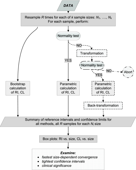
Based on our experience, a flow chart of the resampling process has been designed and is shown in Fig. 1. This flow chart implies random samples drawn from the original data for the list of sample sizes. This list should range from relatively low sample sizes up close to the size of the original data. For each size, some large number of random samples (for example, 500) should be drawn without replacement (random sampling with replacement diminishes chances to draw Gaussian-like distribution by potentially repeating the same observed values). For each sample, different RI calculation methods should be applied: a bootstrapping, parametric (if the sample distribution passes the normality test), or some kind of transformed parametric method, including a normality test for transformed data and backward transformation of the results. If the sample passes the normality test, no transformation should be performed. Some samples could miss both parametric and transformed parametric results. Ideally, several different transformations should be used from the beginning. The choice of the transformation method is determined by its applicability to the original observed data. All calculations should be done with the same transformation method (or set of methods) for all samples, where applicable.

FIG. 1.

Algorithm of the resampling procedures for the selection of RI calculation method. (If neither the drawn sample nor the transformed sample passes the normality test, only bootstrap results are collected for that sample.)

Finally, data on RI with 90% CL should be collected and presented as box plot graphics for each method and each sample size. The method providing the minimal sample size bias along with the fastest sample size convergence and the lowest CL should be chosen to generate an RI and a CL for clinical use. Clinical considerations must also be taken into account.

The flow chart described above was implemented in the program codes written with R software. These codes are available to interested researchers upon request.

RESULTS

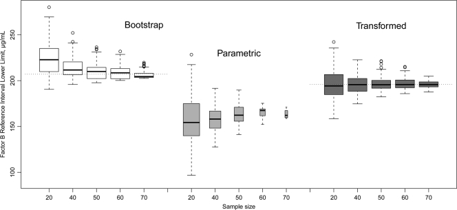
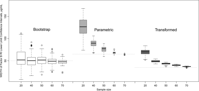
Data for resampling drawn from 81 factor B calculations are presented in Fig. 2 and 3. The distribution of the factor B observations was not Gaussian (Shapiro-Wilk normality test P value of <0.001). An analysis of the resampling from that set showed that the bigger the sample size was, the less the proportion of samples was normally distributed. For instance, sampling by 20 observations generated 74% normally distributed sets; sampling by 40 observations generated 36%; sampling by 50 points generated 24%, etc. This observation is represented by the width of the box plots in Fig. 2 and 3. The percentage of normally distributed, log-transformed subsets was 98% for a sample size of 20, 99% for a sample size of 40, and 100% for larger sample sizes.

FIG. 2.

Effect of sample size on RI lower bound, complement factor B data. Dotted horizontal lines indicate lower limit of RI for the original population (81 observations). Box plots show the first, second, and third quartiles, with whiskers extended to the most extreme data point, which is no more than 1.5 times the IQR from the box. Points exceeding 1.5 times the IQR are shown. The box width is proportional to the square root of the sample size.

FIG. 3.

Effect of sample size on the width of CL for the RI lower bound, complement factor B data. Dotted horizontal lines indicate the width of the CL for the RI lower bound of the original population (81 observations). Box plots show the first, second, and third quartiles, with whiskers extended to the most extreme data point, which is no more than 1.5 times the IQR from the box. Points exceeding 1.5 times the IQR are shown. The box width is proportional to the square root of the sample size.

The values of the RI and the CL determined by different statistical methods are shown in Table 1. To illustrate the variability of the RI, the RI presented in the manual for the factor B assay kit (The Binding Site, Inc.) and the Associated Regional and University Pathologists (ARUP) RI values established for different platform are also shown. Simple bootstrap values for the RI are the same as simple quantiles except that bootstrapping provides evaluation for CL. Bootstrap-derived RI values are biased at low (<50) sample sizes. The results from the log-transformed parametric calculations were chosen as the final RI parameters of the assay. This method generated an unbiased RI and the lowest CL and IQR (see Fig. 2 and 3).

TABLE 1.

Results of complement factor B RI calculation by different methods

Test	RI in μg/ml (90% CL)
	Lower limit	Upper limit
The Binding Sitea	205	400
Current ARUPb	200	510
Transformed parametric	196 (179-214)	589 (539-643)
Parametricc	151 (119-184)	555 (523-588)
Quantiles (0.025, 0.975)	213	622
Simple bootstrap	213 (180-230)	622 (509-662)
BCa (bias corrected accelerated) bootstrap	207 (180-230)	597 (509-662)

^aData were obtained from 29 British blood donors; samples were provided by the manufacturer for guidance purposes only.

^bARUP Laboratories RI for the Beckman Array instrument.

^cData were not normally distributed; therefore, the method was rejected.

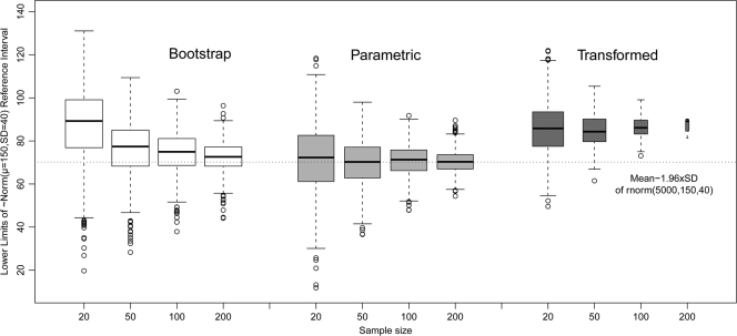
In the second part of the study we investigated the effect of sample size for different RI determination methods using resampling from a large normally distributed computer-generated data set. Summary statistics are presented in Fig. 4. We found that the proportion of log-transformed samples that passed the Shapiro-Wilk normality test diminished with the sample size: 70% with a sample size of 20, 24% with a sample size of 50, 1% with a sample size of 200, and 0% with a sample size of 300 (data not shown). This finding is illustrated by the width of the box plots, which is proportional to the square root of the number of samples in each particular group (see Fig. 4). The fraction of normally distributed subsets drawn from the normally distributed population varied between 94 and 96% for all ranges of sample sizes from 20 to 300.

FIG. 4.

Effect of sample size on the lower limits of RI of 1,000 resamplings without replacement from 5,000 observations of computer-generated Gaussian data ∼N(μ = 150, σ = 40). The dashed horizontal line indicates the original population lower bound (μ − 1.96*σ). Box plots show the first, second, and third quartiles, with whiskers extended to the most extreme data point, which is no more than 1.5 times the IQR from the box. Points exceeding 1.5 times the IQR are shown. The box width is proportional to the square root of the sample size.

As expected, the best method of RI calculation for the normally distributed population was parametric; it was unbiased and had the lowest IQR. Bootstrapping was biased at a low sample size, and log-transformed parametric calculations were heavily biased at all sample sizes.

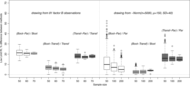
To emphasize the importance of comparison between legitimate methods of RI determination, the resampling data showing the relative differences for RI low limits are presented in Fig. 5. For each random sample drawn, the absolute difference between RI low limits for each pair of methods was divided by the RI low limit value corresponding to the best method for that data set involved in the comparison. For the factor B data, as indicated above, the best method was the transformed parametric, and the next best method was bootstrapping. For the Gaussian population, the best method was the parametric, and the next best one was the bootstrapping.

FIG. 5.

Relative differences of RI lower limit determination using different methods. (Left panel) Sampling from 81 factor B observations (200 drawings for each sample size). (Right panel) Sampling from a normally distributed computer-generated population of 5,000 (1,000 drawings for each sample size). The box plot width does not represent the number of values in each set. Abbreviations: B, bootstrapping; P, parametric; T, transformed parametric calculations. Denominators are the values for the best method for the corresponding original data set (factor B or Gaussian distribution).

DISCUSSION

The CLSI recommends collecting at least 120 specimens for RI determination. After sorting the data, the third extreme values from both ends can be used as the lower and upper RI (95% central interval) without any calculations, and 90% confidence intervals fall within the ranked values (the CL for the lower RI are values 1 and 7, and the CL for the upper RI are 114 and 120). According to the corresponding table in reference 1, for sample sizes from 119 to 187, 90% CL include extreme values: the minimum and maximum. Obviously, it makes the determination of 90% CL highly sensitive for outliers. The simplicity of the CLSI-recommended rank-based procedure for the RI calculation does have risky aspects.

Different approaches to RI calculation produce different results (as illustrated in Table 1 for the factor B assay, and in Fig. 5 for the resampling simulations). The use of a single approach for RI calculation can lead to inaccurate RI determination. Differences could easily be as high as 20%.

Parametric methods assume ideal symmetrical Gaussian distribution of data. However, this parametric methodology is not always applicable because the data are seldom normally distributed. This was the case of sampling from factor B values in the present study. Transformed parametric calculation of RI is often used to overcome this problem. As shown in the present study, log transformation of factor B observations generated Gaussian distributions in almost 100% of all sets. More importantly, in this particular case, log transformation was not biased by the sample size, and the spread of the RI lower limits for different sample sizes was the lowest, compared to parametric and bootstrapping computations.

The use of data transformation for RI calculation as an initial approach is also not always recommended. As illustrated in Fig. 4, when log transformation was applied to the simulated data taken from a large normally distributed population, it produced heavily biased lower RI values and did not converge to the population lower RI limit when sample size increased. In this case, the use of parametric methods was preferable, with no sample-size-biased RI determinations and minimal IQR. Thus, data transformation should not be used as a default without analyzing the original distribution of the data.

Although once considered computationally intensive, bootstrapping methods are now ubiquitous in quantitative science. This is because bootstrapping methods are nearly free of assumptions about data distribution, and they use data-driven statistics, as opposed to formula-driven methods. These methods still need special software packages, but as they have been gaining users, they are becoming increasingly available in standard quantitative packages. As shown here, the use of bootstrap methods for RI and CL calculations was not the best overall method, but in both cases bootstrapping provided nicely converging determinations that were close to the best methods. However, it should be noted that when only small sample sizes are available for RI determination (say, less than 50 observed values), bootstrapping methods should be used cautiously, because they could produce biased parameter estimates.

The results of the present study support the recommendation to use and compare a variety of approaches for RI calculations. We believe that resampling simulations can help researchers make the right choice of the calculation method. The determination of RI and CL is a critical issue in the clinical interpretation of laboratory test results. We hope that our work will attract more attention to this problem. For those who are able to allocate more time and effort to this issue, our work could serve as a starting point or could even lead to new directions in investigation.

REFERENCES

- 1.Box, G. E. P., and D. R. Cox. 1964. The analysis of transformations (with discussion). J. R. Stat. Soc. Ser. B 26:211-252. [Google Scholar]
- 2.Box, G. E. P., and P. W. Tidwell. 1962. Transformation of the independent variables. Technometrics 4:531-550. [Google Scholar]
- 3.Carpenter, J., and J. Bithell. 2000. Bootstrap confidence intervals: when, which, what? A practical guide for medical statisticians. Stat. Med. 19:1141-1164. [DOI] [PubMed] [Google Scholar]
- 4.Chernick, M. R. 2008. Bootstrap methods: a guide for practitioners and researchers. Wiley-Interscience, Hoboken, NJ.
- 5.Clinical and Laboratory Standards Institute. 2008. Defining, establishing, and verifying reference intervals in the clinical laboratory. CLSI approved guideline C28A3E, 3rd ed. CLSI, Wayne, PA.
- 6.Davison, A. C., and D. V. Hinkley. 1997. Bootstrap methods and their applications. Cambridge University Press, Cambridge, United Kingdom.
- 7.Efron, B., and R. Tibshirani. 1991. Statistical data analysis in the computer age. Science 253:390-395. [DOI] [PubMed] [Google Scholar]
- 8.Friedberg, R. C., R. Souers, E. A. Wagar, A. K. Stankovic, and P. N. Valenstein. 2007. The origin of reference intervals. Arch. Pathol. Lab. Med. 131:348-357. [DOI] [PubMed] [Google Scholar]
- 9.Henderson, A. R. 2005. The bootstrap: a technique for data-driven statistics. Using computer-intensive analyses to explore experimental data. Clin. Chim. Acta 359:1-26. [DOI] [PubMed] [Google Scholar]
- 10.Henderson, A. R. 1993. Chemistry with confidence: should clinical chemistry require confidence intervals for analytical and other data? Clin. Chem. 39:929-935. [PubMed] [Google Scholar]
- 11.Horn, P. S., and A. J. Pesce. 2003. Reference intervals: an update. Clin. Chim. Acta 334:5-23. [DOI] [PubMed] [Google Scholar]
- 12.Horn, P. S., A. J. Pesce, and B. E. Copeland. 1998. A robust approach to reference interval estimation and evaluation. Clin. Chem. 44:622-631. [PubMed] [Google Scholar]
- 13.Linnet, K. 2000. Nonparametric estimation of reference intervals by simple and bootstrap-based procedures. Clin. Chem. 46:867-869. [PubMed] [Google Scholar]
- 14.Solberg, H. E. 2007. Establishing and use of reference values, p. 229-238. In C. A. Burtis, E. R. Ashwood, and D. E. Bruns (ed.), Tietz Fundamentals of clinical chemistry, 6th ed. Elsevier Saunders, St. Louis, MO.