Space-time latent component Modeling of Geo-referenced health data

Abstract

Latent structure models have been proposed in many applications. For space time health data it is often important to be able to find underlying trends in time which are supported by subsets of small areas. Latent structure modeling is one approach to this analysis. This paper presents a mixture-based approach that can be appied to component selction. The analysis of a Georgia ambulatory asthma county level data set is presented and a simulation-based evaluation is made.

1 Introduction

In the analysis of geo-referenced health data, it is commonly found that models for relative risk are structured around additive risk components (see e.g. [1, 2]). These components are often assumed to be random effects. While these models provide parsimonious descriptions of risk variation, they do not provide information directly about between area structure in terms of localized differences in behavior. In the spatiotemporal domain, the extension of the spatial component into sequences of disease maps leads to new temporally-referenced components being added to the random effect set. In what follows, we will confine our discussion to a commonly occurring format for space-time disease data: counts observed within small arbitrary geographical areas (census tracts, counties, zip codes etc.) and also fixed time periods. Various authors have proposed random effect models for relative risk estimation in such situations ([3], [4], [5], [2], [6], [7], [8], [9], [10]). In general, random effect models attempt to mimic the underlying smooth variation in risk by using global parameterization of the model. This implies, for example, that one spatially-structured random effect describes all the regional spatially-structured behavior. Here, we attempt to describe the overall level of risk in space-time via an interaction of spatial and temporal latent effects. In this sense, our models differ substantially from those previously proposed as they have a non-fixed mixture formulation which is meant to allow the decomposition of the overall risk into groups of effects defined by spatial location. Alternative ST modeling approaches are described in [11], [12] and [13]. An evaluation of conventional space-time random effect models is given in [14].

The development is presented as follows. In section 2, we present the interaction latent variable space-time model. In sections 3 and 4, we develop the Bayesian implementation via posterior sampling. Following that, we present the application of the approach to a county level ambulatory care sensitive asthma dataset from the state of Georgia USA, and then in section 6, we consider a simulation-based evaluation of the capabilities of the method. Finally, we conclude with general discussion of the approach and future directions for development.

2 Model Development

Given a set of spatial and temporal observation units, we wish to model temporal variations that are disaggregated by region. Essentially, we believe that underlying the map sequence (evolution), there are some temporal effects expressed by only some subsets of regions. Notice this is not the same as assuming that there are geographically-varying regression parameters ([15]) or that classification tree structures are being estimated ([16]).

Define the count of disease (incident, prevalent or mortality) within an observation unit as y_ij where i = 1, …., m small (geographic) areas and j = 1, …‥, J time periods. The units are assumed to be non-overlapping. We make the common assumption that at the 1st level of the hierarchy the data have a Poisson distribution with expectation μ_ij, i.e.

$$y_{ij}\sim \mathit{\text{Pois}}({\mu }_{ij}),$$

where μ_ij = e_ij·η_ij and e_ij is the expected count and η_ij the relative risk in the i – j th unit. While this assumption is convenient in the analysis of disease count data, it is possible to generalize this in our approach. This is discussed further in a later section. We focus here on the modeling of the relative risk parameter η_ij. In practical applications, the specification of e_ij will be important, of course, but our focus here is on the modeling of the relative risk component. In our approach, we assume that the log relative risk consists of three components : a predictor which is a function of fixed covariates, a function of random effects and a mixture term that describes how regions relate to different temporal components. This can be defined in its most general form as,

$$log{\eta }_{ij}=x_{ij}^{\prime }{\beta }_j+z_{ij}^{\prime }\gamma +{\Gamma }_{ij}$$ (1)

where $x_{ij}^{\prime }$ is a vector of covariate values for the i th area at the j th time period, β_j is a parameter vector indexed by the time period, $z_{ij}^{\prime }$ is a vector of random effect values for the i th area and j th time period and γ is a unit vector and the term Γ_ij is a mixture component which is also indexed for the i th area and j th time period. In general, conventional space-time random effect models often assume the first two of these components to allow for covariate effects (often social deprivation, or spatial trend components), and random effects (unobserved confounding or heterogeneity). These effects are usually globally-defined (i.e. controlled by global parameters for the whole map or time period). In what follow, bar an intercept term, we will focus only on models including the last term (Γ_ij). Discussion of the implication of fitting both $z_{ij}^{\prime }\gamma$ and Γ_ij in terms of identification is discussed briefly at the end of this paper.

2.1 Mixture specification

The component Γ_ij should be designed to disaggregate the temporal variation and associate different forms with the spatial features. To this end, a variety of approaches have been proposed. For example, [17] and [18] described a factor analytic approach to the specification of spatial latent structure where the mean structure of the model consists of functions of loadings and their associated factors. The factors have spatial labeling, i.e. g(θ_ij) = μ_j + λ_jf(s_i) where j denotes the variable and i the observation unit and s_i the spatial location. Alternative specifications have been suggested by [19], and [20]. While factor analysis provides a useful mechanism to yield orthogonal components it is sometimes preferred to have components which do not require such constraints. It is possible that components could be regarded as being attached to areas and these areas form groups. In that case, a mixture approach can be considered.

In our development, we assume a linear predictor as in (1) but with the specification

$${\Gamma }_{ij}={\alpha }_0+{\mathbf{\text{w}}}_{ij}^{\prime }{\mathit{\chi }}_j.$$

Here we assume there are l = 1, …, L underlying components. We consider temporal components χ_j : {χ_1j, …., χ_Lj}′, where χ is an L × J matrix of unobserved temporal components {χ_lj}. In addition, we assume that each region of the spatial map can have a (possibly time-varying) weight for each component :w is a L × m × J weight matrix, with element w_lij. These two components form the basis of the mixture model. As can be seen, when written by element: ${\mathbf{\text{w}}}_{ij}^{\prime }{\mathit{\chi }}_j=\mathbf{\text{∑}}_{l=1}^L{w}_{\mathit{\text{lij}}}\cdot {\chi }_{lj}$, this linear combination describes underlying temporally-varying components where a spatially-dependent weight ‘votes’ for each component. In addition, the weight can be time-dependent. In what follows, we do not examine the time dependence of weights and so we focus on ${\mathbf{\text{w}}}_i^{\prime }$. This has advantages, in particular as it provides for greater identification of components.

2.2 Properties of χ and w

2.2.1 Temporal components

The temporal components in this model are defined by a prior distributional structure that provides for time dependence. We would like to allow smooth temporal variation but do not want to restrict this variation too much. A joint specification for the temporal components is considered here where the vector of components χ_j has a multivariate Gaussian distribution with

$${\mathit{\chi }}_j\sim N_L(\mathit{\rho }\cdot {\mathit{\chi }}_{j-1},\Psi )$$

where N_L(a, B) denotes a L-component multivariate Gaussian distribution with mean vector a and L × L covariance matrix B, and · denotes a Schur product. This is an autoregressive formulation with the smooth transition between time points governed by the autoregression dependent on a single time lag. The parameter vector ρ controls the strength of dependency on the previous value and has dimension L. The choice of the ψ matrix may have import in the ability of computational algorithms to detect distinct components. Our first assumption regarding this matrix is that we assume it is constant in time. This is a reasonable assumption given that we allow variation over time in the components. This also helps to provide for identification of the temporal components. Alternatives exist of course such as block diagonal covariances. We do not consider these here.

Hence, we initially choose to define a Gaussian autoregressive dependence on the component :

$$\begin{array}{cc}{\chi }_{lj}\sim N({\rho }_l{\chi }_{lj-1},{\tau }_{{\chi }_l})& {\forall }_l\end{array}.$$

This specification allows for dependence while also allowing the separate specification of a precision parameter ${\tau }_{{\chi }_l}^{-1}$. Note that a different precision parameter is allowed for each component. This corresponds with a simple diagonal covariance matrix of the form τ_χ · I, where I is a unit matrix. A log transformation can also be used to ensure positivity. An alternative possibility for this lag dependence would be a gamma distribution such as

$$\begin{array}{cc}{\chi }_{lj}\sim \mathit{\text{Ga}}(c_l{\chi }_{lj-1},c_l)& {\forall }_l\end{array}.$$

As these temporal components are not observed, we need to make assumptions about their form. First, it is important not only to specify the form of temporal dependence, but it is also important to specify how these components will relate to each other. Here, we don't want to impose unnecessary restrictions on the time components, such as orthogonality. For example, it is of course conceivable that components could cross over each other in some applications where spatial disaggregation is the focus. On the other hand, it may be reasonable to assume that components must be distinct, if simply from a standpoint of computational efficiency. For the precision components, we assume conventional uniform distributions on σ_l, such as σ_l ∼ U(0, c) where ${\tau }_{{\chi }_l}={\sigma }_l^2$ and c is a constant (see Section 3).

2.2.2 Spatial weights

Region specific weights w_lij are relative measures of component contribution to each region, which satisfy two conditions, w_lij > 0 and ${\mathbf{\text{∑}}}_{l=1}^L{w}_{\mathit{\text{lij}}}=1$. Hence the weights have a probability distribution across the components for a given region and time. To obtain normalization, we assume that $w_{\mathit{\text{lij}}}=\frac{w_{\mathit{\text{lij}}}^{\ast }}{{\mathbf{\text{∑}}}_{l=1}^L{w}_{\mathit{\text{lij}}}^{\ast }}$, and proceed to model $w_{\mathit{\text{lij}}}^{\ast }$. We can assign a range of distributions for the un-normalized weights $\{w_{\mathit{\text{lij}}}^{\ast }\}$. Note that, in general, we might want to model both spatial and temporal variation in the weights. Here, we will focus on the spatially-dependent weights and we drop the temporal subscript for convenience. The weights should be positive and so a suitable distribution could be a log-normal prior distribution to $w_{li}^{\ast }$:

$$w_{li}^{\ast }\sim ln\left({\alpha }_{1li},{\tau }_w\right).$$

For the prior distribution of un-normalized weight means α_1li, we can consider a variety of full MVN prior models or Markov Random field models which allow spatial correlations between weights of different components:

$${\alpha }_{1li}\sim \mathit{\text{MV}}{N}_{\mathit{\text{mL}}}({\pi }_{1li},\Phi ).$$

For convenience, the conditional autoregressive prior distribution is assumed here

$${\alpha }_{1li}|\{{\alpha }_{1l,-i}\},n_i,{\tau }_{{\pi }_{1l}}\sim N({\overline{\alpha }}_{1li},\frac{{\tau }_{{\alpha }_{1l}}}{n_i}),$$

where {α_1l,−i} = (α_1l1, ⋯, α_1l,i−1, α_1l,i+1, ⋯, α_1lm)^T, n_i is the number of neighbors of site i, τ_α1 is the conditional variance of α_1li, and ${\overline{\alpha }}_{1li}={\mathbf{\text{∑}}}_{i\in {\partial }_i}\frac{{\alpha }_{1li}}{n_i}$, the average of the neighboring values (∂_i is the neighborhood of site i). As will be seen later we can in fact extend the single field CAR model as the weight fields {α_1li} can be considered to be cross-correlated. This can be accommodated via a multivariate CAR specification. The Multivariate intrinsic CAR model ([21]) has the capability to allow for correlation to be specified between the spatially structured components of different spatial fields. Define α_1i = (α_1li, ⋯, α_1Li). The MCAR is defined as,

$${\mathit{\alpha }}_{1i}|{\mathit{\alpha }}_{1-i}\sim N(B_{ii}^{-1}\mathbf{\sum }_{j\ne i}-B_{ij}{\mathit{\alpha }}_{1j},B_{ii}^{-1}),$$

where α_1−i = (α₁₁, ⋯, α_1i−1, α_1i+1, ⋯, α_1L) and $B_{ii}^{-1}{\mathbf{\sum }}_{j\ne i}-B_{ij}$ is a L × 1 vector of sum of the weighted neighboring values. B_ij is the ijth L × L block of the IL × IL symmetric positive definite matrix B which is defined by the adjacency matrix C and variance matrix Σ,

$$\mathbf{\text{B}}={\mathbf{\text{∑}}}^{-1}(\mathbf{\text{I}}-\mathbf{\text{C}}),$$

where Σ⁻¹ and C are IL × IL matrix which satisfy the condition $C_{ij}{\mathbf{\text{∑}}}_j={\mathbf{\text{∑}}}_i{C}_{ji}^T$. We denote this specification as MCAR(Σ).

As an alternative specification, a Dirichlet prior distribution may be substituted for the prior distributions of weights by assigning Gamma distributions to $w_{li}^{\ast }$.

$$w_{li}^{\ast }\sim G({\alpha }_{1li},1)$$

where α_1li is the parameter that is not temporally-dependent but varies over space. This provides for a simple alternative which does not involve any prior spatial dependence.

2.3 Estimation of number of components

In the simplest model, the number of components (L) is assumed fixed, which is appropriate when the number of components is known. However, in general, the number of components is not known, and must be estimated. There are several different approaches to estimation of the number of components. One common way is to compare a range of models with different fixed number of components via posterior probability, BIC, Bayesian model averaging, or DIC to assess goodness-of-fit, and decide the number of components by choosing the best model based on several criteria. This approach might be easy to conduct when we assume the component number is small. However, when we expect large numbers of components, comparing every possible model with some criterion would be very inefficient, and another simple approach is required. Another approach is to use reversible jump MCMC to estimate the component number and components based on samples from the joint posterior of the component number and components within a Bayesian framework. Although this approach provides a more efficient way to estimate the component number than the previous approach, reversible jump MCMC in general still requires computational intensiveness and usually requires purpose-written software implementation. In our model, we suggest a simple approach to the estimation of the component number by introducing an entry parameter to each component which describes the presence or absence of the components (see e.g. [22]). This entry parameter method is, in fact, a special case of reversible jump MCMC, which can be easily implemented without additional software development. By using entry parameters, each component has a chance of being sampled at each iteration, and the presence of components are determined based on the average posterior distributions of entry parameters. The approach requires the introduction of a ‘full model’ with a large number of L components. Considering the entry parameters, the mixture component is defined as,

$${\Gamma }_{ij}={\alpha }_0+\mathbf{\text{∑}}_{l=1}^L{\psi }_l{w}_{il}{\chi }_{lj}$$ (2)

where ψ_l is an entry parameter ([23]). Other variants of this approach are found in [24]. For the prior distribution of ψ_l, we consider the Bernoulli distribution with probability p_l,

$${\psi }_l\sim \mathit{\text{Bern}}(p_l).$$

This allows the component to enter the model with probability p_l. The Bernoulli probability can also have a hyper-prior distribution or could be considered constant (0.5 being an non-informed guess). If a hyperprior were assumed then a beta distribution would be a conventional choice.

3 Bayesian implementation

For the purposes of exposition, in what follows we focus on models without covariates or additional random effect terms. These can be added in a straightforward manner in a given application. We also have found that much extra-variation is accounted for by mixture components and these models can yield better goodness-of-fit diagnostics than random effect models (see an example of this in Section 7). In the Bayesian implementation, statistical inference is based on Markov chain Monte Carlo samples, generated from a posterior distribution. The likelihood for the model specified above can be written in the general form

$$L(\mathbf{\text{y}}|\cdot )=\prod _{i=1}^m\prod _{j=1}^J\mathit{\text{Po}}(y_{ij}|e_{ij},{\alpha }_0,w_{\mathit{\text{lij}}},{\chi }_{lj}).$$

The Bayesian model specification is completed by assigning prior distributions to each parameter. The intercept parameter (α₀) will be assumed to have a highly dispersed zero-mean Gaussian prior distribution:

$${\alpha }_0\sim N(0,{\tau }_{{\alpha }_0}),$$

where τ_α0 is the variance of the Gaussian distribution. For the variance parameters (τ_α0, τ_χl, τ_w), we will consider uniform prior distributions for the standard deviations,

$$\{\sqrt{{\tau }_{{\alpha }_0}},\sqrt{{\tau }_{{\chi }_l}},\sqrt{{\tau }_w}\}\sim U(0,c),$$

where c is a constant ([25]). For Σ in the MCAR model, we assign a Wishart distribution (Wishart(R⁻¹, r)) where R is a m × m dimensional positive definite matrix and r is a degree of freedom. Beta prior distributions are assigned to the temporal dependency parameter (ρ) in the latent parameter and the Bernoulli probability (p_l) which is associated with the entry parameter.

$$p_l\sim \mathit{\text{Beta}}(d,d).$$

The choice of d = 1 yields a uniform prior distribution.

The full posterior distribution obtained based on the likelihood and prior distributions is defined as,

$$P({\alpha }_0,\mathit{\beta },\mathbf{\text{w}},\mathit{\chi },\mathbf{\text{p}})=L(\mathbf{\text{y}}|\cdot )p({\alpha }_0|{\tau }_{{\alpha }_0})p(\mathbf{\text{w}}|{\mathit{\alpha }}_1,{\tau }_w)p({\mathit{\alpha }}_1|{\mathit{\tau }}_{{\alpha }_1})p(\mathit{\chi }|\mathbf{\Psi },\mathit{\rho })p(\mathit{\rho })p(\mathbf{\text{p}})\mathbf{\text{p}}(\mathbf{\tau })p(\mathbf{\text{∑}}),$$

where y = (y₁₁…., y_mJ)^T, w = (w₁, …., w_m)^T, α₁ = (α₁₁₁₁, …., α_1LmJ)^T, χ = (χ₁₁, …., χ_LJ)^T, ρ = (ρ₁, …., ρ_L)^T, p = (p₁, …., p_L)^T, τ_α1 = (τ_α11, …., τ_α1L)^T, ψ_ii=(τ_α0, τ_w, τ_χl)^T.

Samples are generated from the posterior distribution using several sampling algorithms such as Gibbs and Metropolis via adaptive rejection sampling. The Gibbs sampling method is applied to the variance parameters (τ) for τ_u, τ_υ, τ_α0, τ_α*, τ_χl, τ_w (in the form of standard deviations). For other parameters, Metropolis adaptive rejection sampling method are applied, since the conditional distributions are not easy to sample from, in general.

4 Model comparison

Bayesian model comparison has been examined via a range of measures both predictive and otherwise. Our primary measure is the Deviance Information Criterion (DIC) which is based on the posterior distribution of the deviance function,

$$D(\theta )=-2\mathit{\text{logL}}(\mathit{\text{data}}|\theta ),$$

where L(data∣θ) is the likelihood function for the observed data given the parameter θ ([26]). The DIC considered here is the standard DIC composed of D̄ which measures the model fit and p_D which penalizes overfitting by measuring the model complexity,

$$\mathit{\text{DIC}}=\overline{D}+p_D.$$

D̄ is the mean posterior deviance defined by,

$$\overline{D}=E_{\theta |y}(D),$$

and p_D represents the effective number of parameters defined by,

$$p_D=E_{\theta |y}(D)-D(E_{\theta |y}(\theta )).$$

The DIC evaluates models by measuring the goodness of fit in terms of the overall fitting of the model. Variants of the basic DIC measure have been proposed (see for example [27]) and we will examine two variants here in conjunction with the basic measure. In mixture models, there is a concern that the standard DIC measure does not properly reflect the correct effective number of parameters ([28]). In that case, it is useful to try to estimate this penalty using alternative specifications. Here we examine two additional estimates of the effective number of parameters suggested by [28]: the penalized expected deviance (L^e) and the corrected DIC (DIC_c). In the first case we have L^e = D̅ + p_opt where p_opt was computed via importance sampling based on the output from two chains. In the second case, we assume a corrected DIC of the form DIC_c = D̅ + Σ_j Σ_ip_Dij and compute the p_Dij from the double chain output.

The DIC criterion does not reflect on the prediction performance in the evaluation, and it is useful to examine another criterion to compare models in terms of the prediction performance. The mean squared prediction error is another criterion which measures prediction performance by comparing observed values and prediction values, which is defined by,

$$\mathit{\text{MSPE}}=\mathbf{\text{∑}}{(y_{ij}-y_{ij}^{pr})}^2/N,$$

where y_ij is the observed value, $y_{ij}^{pr}$ is the predicted value obtained from (2) in posterior sampler output, and N is the number of samples.

5 Data example: Georgia Ambulatory case sensitive asthma

In this example, counts of ambulatory case sensitive asthma in the 159 counties of Georgia were available from the public access health information system OASIS (Georgia Division of Public Health: http://oasis.state.ga.us/) for the years 1999 to 2006. There are 159 small areas (counties) and 8 time periods (years). The counts of asthma were obtained from OASIS and expected rates were obtained from the statewide rates broken by age and gender. For each area the total expected count summed over all age and gender strata was used. Figure 1 displays the standardized incidence ratios for 80 counties (left panel) and the remaining 79 counties (right panel) in alphabetical order.

Figure 1.

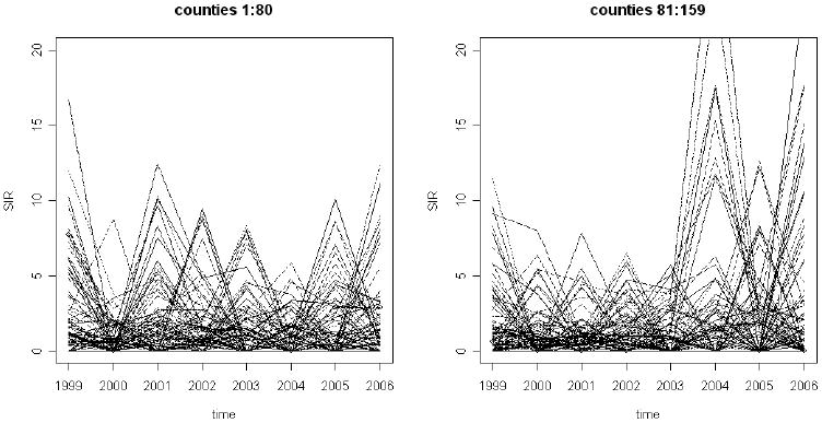
The state of Georgia county level standardized incidence ratios for ambulatory asthma for the period 1999- 2006. Left panel: first 80 counties (in alphabetical order); right panel: remaining 79 counties (in alphabetical order).

Figure 2 displays a selection of standardized incidence maps for the 159 Georgia counties.

Figure 2.

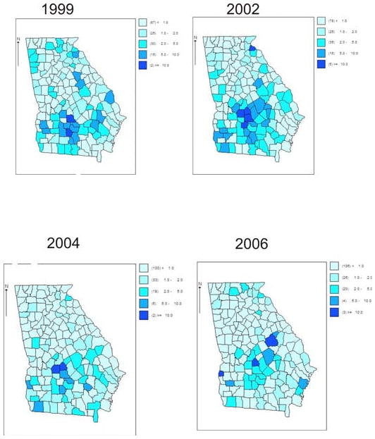
A selection of four years of standardized incidence maps of county level ambulatory sensitive asthma in Georgia (1999, 2002, 2004, 2006).

Using the Georgia ambulatory case sensitive asthma data, we explored various models that we proposed in the previous section. Extensive exploratory examination of the data suggest that a small number of components would usually suffice to capture the disaggregated temporal variation across space. Hence, in this example we have fitted full models with L = 4 components. Larger component numbers were examined but found to yield a poorer fit in general. This choice is a compromise between allowing for disaggreation and searching for a parsimonious fit. We first consider the model with a Dirichlet prior distribution for the weights w_li by assigning Gamma distributions to un-normalized weight $\left\{w_{li}^{\ast }\right\}$, and we denote this model as Model 1:

$$\begin{array}{l}{y}_{ij}\sim \mathit{\text{Pois}}(e_{ij}\cdot {\eta }_{ij})\\ log{\eta }_{ij}={\alpha }_0+{\mathbf{\text{w}}}_{ij}^{\prime }\mathit{\chi }\\ w_{li}=\frac{w_{li}^{\ast }}{{\mathbf{\text{∑}}}_{l=1}^L{w}_{li}^{\ast }}\\ w_{li}^{\ast }\sim G(1,1).\end{array}$$

In model 1, there is no consideration of the spatial structure of the weights and it is possible to extend the model by modeling spatial structure in the weight prior distributions. The next model we applied to our data is a model with log normal distribution and multivariate intrinsic CAR distribution (MCAR) for un-normalized weights $\left\{w_{li}^{\ast }\right\}$ to allow a spatially correlated effect in the mean of the weights. For the hyper prior distribution of Σ_α1, we assign the Wishart distribution, Wishart(R⁻¹, r) where R⁻¹ is a diagonal matrix with an element 0.01, and r is the number of latent components. This model is denoted as Model 2:

$$\begin{array}{l}{w}_{li}^{\ast }\sim ln({\alpha }_{1li},{\tau }_w)\\ {\alpha }_{1i}\sim \mathit{\text{MCAR}}({\mathbf{\text{∑}}}_{{\alpha }_1}).\end{array}$$

In the previous two models, weights associated with latent factors are assigned to any value between 0 and 1 and all latent components are involved in modeling the mean of the Poisson model. Instead of allowing the inclusion of all latent components in the model, we may assume that there is only one dominant latent component that determines the underlying process. In such a situation, the main objective is to find out the particular primary latent component, and we can suggest a model with a singular multinomial distribution for the weights (Model 3):

$$\begin{array}{l}{w}_{li}^{\ast }\sim \mathit{\text{Multi}}(1,p_{li})\\ p_{li}=\frac{p_{li}^{\ast }}{{\mathbf{\text{∑}}}_{l=1}^L{p}_{li}^{\ast }}\\ p_{li}^{\ast }\sim G(1,1).\end{array}$$

This model allows there to be an assignment to a single component. To allow for the spatially correlated effects in p_li, we can also assign a multivariate intrinsic CAR (MCAR) distribution for the mean of $log(p_{li}^{\ast })$ (Model 4):

$$\begin{array}{l}{w}_{li}^{\ast }\sim \mathit{\text{Multi}}(1,p_{li})\\ p_{li}=\frac{p_{li}^{\ast }}{{\mathbf{\text{∑}}}_{l=1}^L{p}_{li}^{\ast }}\\ p_{li}^{\ast }\sim ln({\alpha }_{1li},{\tau }_w)\\ {\alpha }_{1i}\sim \mathit{\text{MCAR}}({\mathbf{\text{∑}}}_{{\alpha }_1})\end{array}$$

In the all models, we assign a random walk Gaussian distribution for the prior distribution to allow the temporal correlated variation of latent components:

$$\begin{array}{cc}{\chi }_{lj}\sim N({\chi }_{lj-1},{\tau }_{{\chi }_l})& {\forall }_l\end{array}.$$

The results of fitting these four different models to the Georgia data is given in Table 1. For the calculation of the DIC and the MSPE, we used two software implementations: WinBUGS and R, in which the p_D is calculated in different ways. While in WinBUGS, the p_D is calculated by the difference between the expectation of deviance and the deviance estimated at the mean of the posterior distribution, (p_D = E_θ∣y(D) − D(E_θ∣y(θ))), in R, the p_D is calculated by the variance of deviance (p_D = var(D)/2). In the case of models with continuous weights (Model 1 and Model 2), the p_D and the DIC is calculated in WinBUGS and for the models with the multinomial distribution (Model 3 and Model 4), the p_D and the DIC are calculated by R. The pD of Model 1 and 2 is calculated by D̅ − D(θ̄), where θ̄ is the posterior mean of θ, and the pD of Model 3 and 4 is var(D)/2. Hence, we can compare model 1 and 2 or model 3 and 4, but we can not compare all models at the same time. The MSPE is a more suitable criterion for general model comparison, albeit predictive comparison. Model 1 which uses a Dirichlet prior distribution for weights shows the lowest MSPE values. The adjusted DICs (L^e, DIC_c) are larger than the standard DIC, which suggests a degree of optimism in the standard DIC, but also tend to support the model 1 as the most appropriate model. It is reassuring that each criterion leads to the same model choice, although the ranking is not completely the same. The DIC_c does not display the same overall ranking as L^e, and model 3 is favored over model 4 by L^e, although model 1 is selected by all the criteria.

Table 1.

The DIC, DIC variants and MSPE results: Model 1 is the model with the Dirichilet prior distribution, Model 2 is the model with the lognormal distribution and MCAR, Model 3 is the multinomial distribution and Model 4 is the multinomial distribution and MCAR for unnormalized weights. For the models 1 and 2, pD = E_θ∣y(D) − D(E_θ∣y(θ)), and in the model 3 and model 4, pD = Var(D)/2. The MSPE is calculated in WinBUGS. The penalized expected deviance (L^e) and corrected DIC (DIC_c) were calculate on R from double chain output.

	pD	DIC	MSPE	Le	DICc
Model 1	207	4070	6.224	4355	4885.8
Model 2	239	4120	6.33	4357	4902
Model 3	104*	5079	7.61	5527	5248
Model 4	101*	5250	7.59	6199	5056

A fixed parametrization does not allow the selection of components within a model and so the then included entry parameters in the models and applied them to our data to test whether the entry parameters improve the goodness of fit or prediction capability. The new formulation is then:

$$\begin{array}{l}{y}_{ij}\sim \mathit{\text{Pois}}(e_{ij}\cdot {\eta }_{ij})\\ log{\eta }_{ij}={\alpha }_0+\mathbf{\text{∑}}_{l=1}^L{\psi }_l{w}_{il}{\chi }_{lj}.\end{array}$$

Table 2 shows the DIC, DIC variants and MSPE results for the entry parameter models. The results demonstrate that the model which uses a Dirichlet prior distribution for weights (Model 1) is the best fit model in terms of the MSPE.

Table 2.

The DIC and the MSPE results with entry parameters: Model 1 is the model with the Dirichlet prior distribution, Model 2 is the model with the lognormal distribution and MCAR, Model 3 is the multinomial distribution and Model 4 is the multinomial distribution and MCAR for unnormalized weights. For the model 1 and 2, pD = E_θ∣y(D) − D(E_θ∣y(θ)), and in the model 3 and model 4, pD = Var(D)/2. The MSPE is calculated on WinBUGS. The Plummer L^e and DIC_c are also shown.

	pD	DIC	MSPE	Le	DICc	Entry components
Model 1	503	5057	6.206	4447	4884	1,2,3,4
Model 2	486	5068	6.52	4692	5231	1,2,3,4
Model 3	78	5447	7.606	6183	5478	1,2
Model 4	77	5503	7.646	8781	5565	1,2

For the models with continuous weights, the 4 latent components are all selected in the model, while when we used the multinomial distributions for the weights, only 2 latent components are selected.

Comparing the DIC and the MSPE after and before applying entry parameters is difficult as the entry parameters are a variable selection tool and must inevitably lead to increased parameterization. Hence direct comparison of DIC between Table 1 and 2 is not appropriate. However, MSPE can be compared directly and it appears that model 1 in Table 2 is smallest overall, followed by model 1 in Table 1. These models both assume a Dirichlet prior distribution for the weight vector. In addition to the standard DIC the variants (L^e, DIC_c) display a similar pattern in that the non-multinomial models are favored and in fact the lowest L^e, or DIC_c is for model 1.

Figures 3, 4 and 5 depict the results of fitting a four component entry parameter model to these data. The model fitted was model 1 in Table 2 which yielded the lowest DIC among the entry parameter models and overall. The model was sampled after convergence (at 100,000 iterations). Convergence genrally takes place much earlier for model 1 and 2 than for models 3 and 4 and so this iteration length is much greater than required. In this case there is a clear selection of two major components: component 1 with a decreasing trend, and component 3 with an increasing trend. The other components are negligible.

Figure 3.

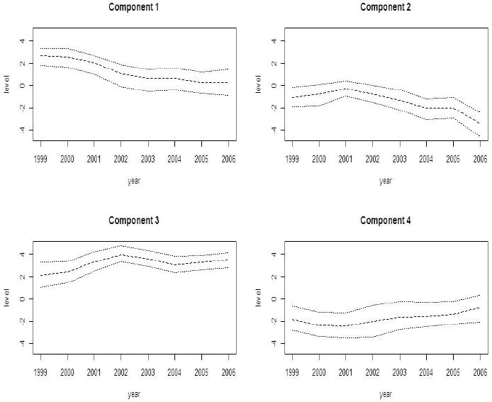
Georgia ambulatory asthma incidence data (1999-2006): posterior expected temporal effects (χ_l) with 95% credible intervals obtained from a converged sampler from an entry parameter model with four latent components.

Figure 4.

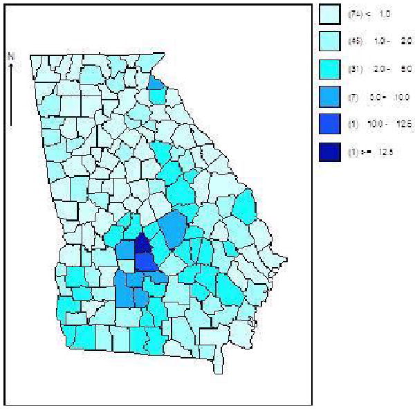
Georgia ambulatory asthma incidence data (1999-2006): posterior mean of relative risks averaged over all 8 time periods for each county for a four component entry parameter model. Clearly displayed is the large cluster of relative risk in Pulaksi and Wilcox counties.

Figure 5.

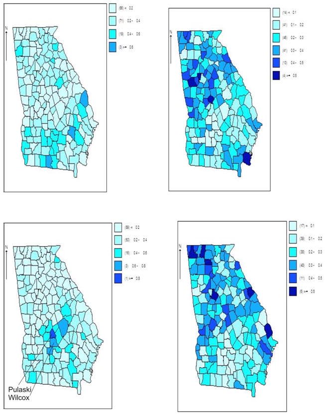
Georgia ambulatory asthma incidence data (1999-2006): posterior expected weight maps for the four components (w_il) from a converged sampler based on a four latent component model. Component 3 has elevated weights for Pulaski and Wilcox counties.

5.0.1 Model fitting and sensitivity

For both data sets we explored a range of models and their sensitivity to prior specification. For example, in both data examples, we examined the effect of removing the entry parameters, and so fitting a full models with maximum number of components. In addition we have examined the effect of changing variance hyperprior specifications, in particular, the range of the uniform specification for the standard deviations. Finally, we have also examined the effect of varying the specification of the Bernoulli entry probability (p_l) when entry parameters are used. In general we have found that across a range of upper uniform limits there was little sensitivity. However for the entry parameter we have found that there is a degree of sensitivity to specification of the entry probability prior distribution. If the parameter is fixed (e. g. at 0.5) there appears to be better recovery than when the parameter is allowed to have a hyperprior distribution.

We have also examined a model where the temporal components have an AR2 Gaussian prior distribution (i. e. χ_lj ∼ N(ρ₁χ_lj−1 + ρ₂χ_lj−2, τ_χ)). This distribution was employed to assess whether additional identification of temporal components would be achieved with such a more flexible assumption. This model, when used with entry parameters, in fact yielded estimated components and weights close to those found for the random walk specification, but yielded a larger DIC measure (by > 40 units). This suggest that a random walk model is likely more appropriate for these data.

In the next section we also report the results of a simulation study designed to assess the identifiability issue of the temporal components as well as model misspecification.

6 Simulation studies

In this section, we present a small simulation study to explore the performance of the space-time latent component models developed in the previous section. The main objectives of our study are to investigate the capability of recovering of true models and the impact of the model misspecification when space-time unobservable latent components exists in the process. We conduct our simulations under two different scenarios, when the number of latent components is known, and when the number of latent components is unknown and needs to be estimated by using the entry parameters. Due to limitations of time, we have restricted our examination to a range of models that provided reasonably good recovery in our example. Hence, here we examine the uncorrelated component and CAR component models, but do not examine the multinomial and multinomial MCAR models. The latter models are discussed further in Section 7.

Simulated counts of disease y_ij over space i and time j are generated from a Poisson model with expected rate e_ij and relative risk η_ij.

$$y_{ij}\sim \mathit{\text{Poisson}}(e_{ij}{\eta }_{ij}),$$

where i = 1, ⋯, I, and j = 1, ⋯, J. For the spatial study region, we use Ohio counties as our spatial test-bed, which consist of I = 88 units, and for the time sequential simulation, we consider 10 time periods. Ohio counties have a regular geography with approximately equal size and shape of counties. The expected rate e_ij at county i and time j is generated from the Poisson distribution with mean 5 and add 1 to each generated expected rate to make it larger than 0. We assume L underlying components, and model the true relative risk η_ij as a function of temporal components and spatially varying standardized weights :

$$\mathit{\text{log}}({\eta }_{ij})={\alpha }_0+{\mathbf{\text{w}}}_i^{\prime }{\chi }_j$$

where w_i is a spatially varying L × 1 weight matrix, and χ_j is a temporally varying L × 1 matrix of unobserved temporal components. α₀ is chosen an appropriate value to restrict the average relative risk to 1 and the relative risk within the range of 0 to 3.5. χ_jl is simulated from a normal distribution with N(ρ_lχ_j−1l, 0.5) to model the temporal dependency of the latent components. We assume ρ_l changes over components, and fix ρ_l to different values which allow different strength of temporal dependency for each temporal component. For the simulation of spatially varying weights, we first generate weight components $w_{il}^{\star }$ from the lognormal distribution with mean α_2il and variance 100 to ensure the positivity of the weight components.

$$\begin{array}{l}{w}_{il}=w_{il}^{\star }/{\mathbf{\text{∑}}}_l{w}_{il}^{\star }\\ w_{il}^{\star }\sim \mathit{\text{ln}}({\alpha }_{2il},100)\end{array}$$

For the spatially correlated weights, α_2il is generated from the normal distribution whose mean is generated from the proper conditional autoregressive model.

$$\begin{array}{l}{\alpha }_{2il}\sim N({\alpha }_{1i},100)\\ {\alpha }_{1i}\sim \mathit{\text{CAR}}(\mathit{\tau })\end{array}$$

where τ is the conditional variance in an improper conditional autoregressive model. In our simulation, we fix τ to be 1. This also allows the addition of extra noise in the weight simulation.

The first part of the simulation is conducted under the scenario that the number of components is known, and addresses the question of how our models can be recovered and what is the impact of misspecification of models. We simulate data from true models with different latent components, and fit the same model (i.e. fitted model = true simulated model) in each case to the simulated data to assess whether different number of latent components affects model recovery. We produced 500 simulated replicate data sets for each simulated model. We consider 2, 4, and 6 latent components, and fix different values for ρ_l, which are defined as ρ₂ = (1, 0.8), ρ₄ = (1, 0.8, 0.6, 0.4) and ρ₆ = (1, 0.9, 0.8, 0.7, 0.6, 0.5), for the 2, 4, and 6 latent component models. To evaluate the capability of recovering of our model, we compare models with the DIC and the mean square prediction error. All of the results displayed are computed from 5,000 iterations after a burn-in of 4000 iterations. Since we estimate several latent components simultaneously, we need to identify the component estimates (χ̅_lj) and associate the component estimates with the true components (χ_lj). This identification of components is done based on the mean square error (MSE). We calculate the MSE of all components for each estimate, and assign a particular component estimate to the true component which yields the minimization of the MSE. In short we computed

$$\mathit{\text{MSE}}=\mathit{\text{ave}}\{min{\mathbf{\text{∑}}_j\left({\overline{\chi }}_{l_j}-{\chi }_{l_j}\right)}^2\},$$ (3)

where χ̅_lj is the posterior mean estimate under the fitted model. We present the identification in Figure 6. Model comparison results of model fitting are done by the average deviance information criterion (ADIC) and the average mean square prediction error (AMSPE) over 500 simulations which are summarized in Table 3. We notice that the ADIC decreases as the number of latent components decreases and the AMSPE decreases as the number of latent components increases. These results indicate the overall fitting is better for the models with fewer latent components, while the prediction capability increases for the models with more latent components. Figure 6 displays the profile plots of estimates of latent components of the model with 6 latent components, based on the minimized MSE in (6). The evidence in this figure suggests that in some cases a reasonably unbiased fit is achieved, but in others (notably factor 1 and 5) there is a poor recovery. This may suggest components are poorly identified in the estimation process. In fact with larger component number the identification can become more problematic especially when an unknown component number is to be estimated. This is discussed in a general context in Section 7.

Figure 6.

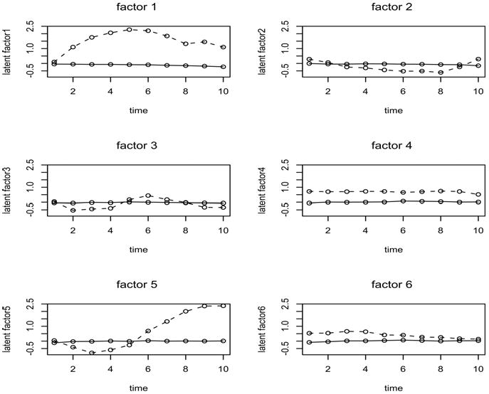
Profile plots of latent component estimators based on the model with 6 latent components. The solid line is the true component and the dotted line is the posterior averaged estimated component.

Table 3.

Model fitting: the average DIC (ADIC), the average pD (ApD) and the average MSPE (AMSPE) over 500 simulations, Model 2: the model with 2 latent components, Model 4: the model with 4 latent components, Model 6: the model with 6 latent components

	ADIC	ApD	AMSPE
Model 2	4019	56	14
Model 4	4087	127	13
Model 6	4185	245	13

We also studied the impact of misspecification of models by fitting models to the simulated data generated from a particular model. Data are simulated from the model with 4 latent components, and simulated data are fitted to the models with different number of components. To assess the impact of spatial correlation of weights on the performance of our models, we also fit the model with uncorrelated weights to the data generated from the model with spatially correlated weights. The uncorrelated weights are generated from the normal distribution with mean 0 and variance 100,

$${\alpha }_{2il}\sim N(0,100).$$

For this assessment 200 simulations were performed. The ADIC and AMSPE of the models were calculated to compare the fitting of models. The results are given in Table 4, which show that the best fit model is the model with 4 latent components and spatially correlated weights based on the ADIC, and the model with 4 latent components and uncorrelated weights also shows similar results. When we fit the models with 6 latent components, we obtain the lower AMSPE than the model with 4 components, which is reasonable due to the contribution of redundant latent components to the prediction of models. However, in terms of the ADIC which is the criterion that penalizes model complexity, we still notice the lower ADIC for the models with 4 components than the models with 6 components, which shows that the DIC would be a good criterion to evaluate the performance of the model. When we compare models with 2 components and 4 components, the ADIC and the AMSPE of models with 2 components are both higher than the models with 4 components, which indicates that models with fewer latent components lead to inefficiency of models in terms of the ADIC and the AMSPE.

Table 4.

Model misspecification: the average DIC and the average MSPE over 200 simulations, Model 2: the model with 2 latent components with spatially correlated weights, Model 4: the model with 4 latent components with spatially correlated weights, Model(U) 4: the model with 4 latent components with uncorrelated weights, Model 6: the model with 6 latent components with spatially correlated weights. Data are generated from Model 4 and fitted by Model 2, Model 4, Model(U) 4, and Model 6.

	ADIC	ApD	AMSPE
Model 2	4509	95	17
Model 4	4086	123	13
Model(U) 4	4087	125	13
Model 6	4155	228	12

In the second part of our simulation study, we considered the situation where the exact number of components is unknown, and needs to be estimated by using the entry parameters. We investigate the performance of the entry parameter in the model for the latent component selection by fitting models with entry parameters of different number of components to the simulated data. We consider models with 4 latent components, and fix various values for ρ_l, which is defined as ρ₄ = (1, 0.7, 0.4, 0.1) to distinguish each component from the others by allowing different temporal dependency of previous values for each latent component. We generate data from the models with 4 latent components and fit entry parameter models with 2, 4, and 6 latent components. For the prior distribution of the entry parameters, we use a Bernoulli distribution with probability 0.5. The evaluation of the performance of entry parameters is done by comparison of models using the DIC and the MSPE. Table 5 presents the estimated number of latent parameters based on the estimated entry parameters when the underlying process has 4 latent components. We accept a latent component in the model if the estimated entry parameter is larger than 0.5. When we fit the entry parameter model with fewer latent components (Model 2) to the data generated from 4 latent components, the 2 latent components are all included in the model. When we apply entry parameter model with 4 latent components (Model 4) to the simulated data using 4 latent components, most cases select the true number of latent components. We also fit the entry parameter model with more latent components than the true number of latent components, and observe that redundant components are selected based on the entry parameters. We compare the performance of different models using the DIC and the AMSPE in Table 6. Based on the DIC, the model with entry parameters of 4 latent components is the best fit model, while the model with entry parameters of 6 latent components shows smaller AMSPE than the other models.

Table 5.

Frequency table of estimators of number of parameters using models with entry parameters with 2, 4, and 6 latent components. the true number of latent components: 4, Model 2: the model with entry parameters of 2 latent components, Model 4: the model with entry parameters of 4 latent components, Model 6: the model with entry parameters of 6 latent components

	2	3	4	5	6
Model 2	200
Model 4	0	8	192
Model 6	0	0	11	103	86

Table 6.

Model fitting with entry parameters with 2, 4, and 6 latent components: the average DIC and the average MSPE over 200 simulations, the true number of latent components: 4

	ADIC	ApD	AMSPE
Model 2	4510	90	18
Model 4	4105	139	14
Model 6	4128	193	13

Summarizing our findings, these simulation results show the importance of the choosing appropriate number of components. Although redundant latent components might improve the accuracy of model in terms of the AMSPE, we conclude that the model with the appropriate number of components is the most efficient model rather than the model with redundant latent components considering the model complexity. Also, the model with fewer latent components does not show better model fit in the respect of the overall model fitting and prediction capability than the model with the appropriate number of components. When we use the entry parameters in the model to estimate the number of latent components, the entry parameters tend to include redundant latent components. However, using the DIC, we can estimate appropriate number of latent components after applying various models with different number of components to data.

7 Discussion, Identification and Conclusions

In this paper we have presented a novel approach to the disaggregation of space-time small area health data via the use of mixture models specified for the mean of the process. We have demonstrated some success in recovering true underlying risk components and stressed the importance of the number of components in this recovery determination. Prior sensitivity has also been examined and we note that the use of a fixed Bernoulli prior parameter (0.5) is preferred compared to the use of a beta hyperprior distribution for the entry parameters modeled. In our real data examples we appear to have recovered components that have 95% credible intervals that do not overlap for a significant portion of the time periods and this suggests strongly that the components are being well estimated. In the Georgia example this is even more evident where there is dramatic separation of the decreasing and increasing trend components.

The generality and usefulness of this approach should also be stressed. Although we have examined small area health data it would certainly be possible to consider other forms of spatiotemporal data such as economic or sociological. Finally to stress the usefulness of the approach, we have also considered a comparison of the method to a conventional random effects model which could be assumed for the Georgia data example. A well-known random effect model, proposed by [2], has been fitted to the Georgia data and overall goodness-of-fit measured with DIC and MSPE. The model consists of separable additive spatial (convolution prior: u_i + υ_i) effects and a temporal effect (random walk prior: γ_j) and an additive ST interaction term (zero-mean Gaussian prior: η_ij). All precisions were assumed to have half-Cauchy prior distributions (as described in Section 3). The relative risk was specified as log θ_ij = α₀ + u_i + υ_i + γ_j + η_ij. The purpose of this comparison is to assess whether a latent effect model could yield a better overall goodness-of-fit than a typical random effect model. In this case, following convergence at 20,000 iterations and based on a sample of 2000, the DIC was 4112 with pD of 339.4 and MSPE of 5.789 for this model. Hence, the mixture model 1 applied to these data yielded a lower DIC (4070) but higher MSPE (6.224) but higher Plummer corrected variants. An additional comparison was made where the ST random effect model was assumed to have a higher order autoregressive prior distribution for the interaction term (second order). In that case the DIC was 4081 with pD =302. While this is a reduction in DIC it remains higher than the model 1 mixture. This stresses the dual ability of these latent models: they can provide estimates of underlying latent components but can also provide a reasonably good overall description of the data themselves.

In all latent structure models the issue of identifiability of components arises. In the model presented here there are two issues. First, as the model allows the estimation of overall small area relative risk it can be seen as a competitor to conventional convolution and fixed component mixture models (e.g. L&C or zip models). In that case the models can be compared without concern about identification of components. In our paper we have demonstrated that the overall goodness-of-fit of the latent model (based on DIC) is comparable to, or can be better than, a commonly used conventional space-time convolution model with uncorrelated interaction (Knorr-Held). Note that there is poor identification of spatial components in that model also, but it can still be used for risk estimation (e.g. [29]). Hence from purely the relative risk estimation point-of-view a latent component model can be beneficial and provide a useful summary of small area risk.

Second, identification affects the estimation of the latent components. In a factor analytic approach to latent modeling and estimation in ST ([17]; [18]; [20]), the orthogonality of components allow for identification. However the disadvantage of this approach is that the interpretation of such decomposition is not simple and could be very difficult in complex real examples (see e.g. [20]). In our models we have temporal components that are naturally interpreted (as a spatial decomposition of an overall temporal series. In our latent model, we approach identification by insisting that the different components have different dependency structures in each dimension. We allow temporal components to intersect which is a natural requirement in real applications. Factor analytic models have somewhat unrealistic assumptions about time dependence of factor effects that make them unattractive in our experience.

Empirical evidence of identification is apparent both in the relatively small standard errors of the estimated components in the real data example (Section 5, Figure 3) and in the simulated examples. The credible intervals for the temporal components do not overlap for the two major components found in the real example (see Figure 3). When components are poorly separated under the simulated true model (Section 6, e.g. Figure 6) then they are poorly estimated. This is to be expected and reflects a lack of separation in the true components. If true components are well separated then we would hope that they could be estimated well. This is in fact the case here as we make the assumption that the temporal components have lag 1 autoregressive prior dependence and the weights are functions of components with spatial structured prior distributions. It is necessary to make these assumptions to guarantee identification. Stronger prior temporal correlation, such as χ_lj ∼ N (α_1lχ_lj−1 + α_2lχ_lj−2, τ _χl) can also be assumed and this would also support strong separation of components ([30], [31]). We aim to investigate some of these assumptions in the future.

In all practical examples examined here, we have assumed that the temporal latent components have only temporal AR dependence, while the spatial weights have spatial dependence only. This both allows the temporal components to gain strength from the multiple time series in the small areas, while the spatial weights gain strength from the temporal repeated measurement in each area.

While computational identification, or lack thereof, could be a problem during sampling ([29]), it has been found to be of limited concern in these applications when samplers are being run over long time periods. It is especially important when CAR models are being employed that longer time is allowed for convergence. Note that for the simple gamma model convergence is often found within a few thousand iterations, and this partly because there are no unit level random effects to estimate in these models.

Models that were not evaluated in our simulation are the more complex multinomial models that fitted poorly in our data example. We would recommend that these models be considered when a categorical selection is the focus.

Finally we should note that we did not consider the inclusion of either covariates in our models nor conventional random effects. We are reassured by the fact that a simple Dirichlet prior distribution for the weights with a random walk Gaussian prior distribution for temporal effects provides a remarkably good fit, compared to more complex models. The addition of covariates to this model is straightforward within the linear predictor, with the caveat that any aliasing with spatial effects modelled in the mixture should be considered ([32]; [33]). The addition of random effects (unstructured or spatially- or temporally-structured) could also be considered. However, this has been avoided in this work so that the ability of a simple mixture model could be evaluated. Clearly an unstructured effect might absorb additional noise, while an structured effect could more likely affect mixture components. Identification of these effects may be problematic in addition, although from a pragmatic viewpoint, if the addition of an effect yields better and parsimonious explanation, then it may be welcomed.

References

- 1.Besag J, York J, Mollié A. Bayesian image restoration with two applications in spatial statistics. Annals of the Institute of Statistical Mathematics. 1991;43:1–59. [Google Scholar]
- 2.Knorr-Held L. Bayesian modelling of inseparable space-time variation in disease risk. Statistics in Medicine. 2000;19:2555–2567. doi: 10.1002/1097-0258(20000915/30)19:17/18<2555::aid-sim587>3.0.co;2-#. [DOI] [PubMed] [Google Scholar]
- 3.Bernardinelli L, Clayton DG, Pascutto C, Montomoli C, Ghislandi M, Songini M. Bayesian analysis of space-time variation in disease risk. Statistics in Medicine. 1995;14:2433–2443. doi: 10.1002/sim.4780142112. [DOI] [PubMed] [Google Scholar]
- 4.Xia H, Carlin BP, Waller LA. Hierarchical models for mapping Ohio lung cancer rates. Environmetrics. 1997;8:107–120. [Google Scholar]
- 5.Knorr-Held L, Besag J. Modelling risk from a disease in time and space. Statistics in Medicine. 1998;17:2045–2060. doi: 10.1002/(sici)1097-0258(19980930)17:18<2045::aid-sim943>3.0.co;2-p. [DOI] [PubMed] [Google Scholar]
- 6.Zhu L, Carlin BP. Comparing hierarchical models for spatio-temporally misaligned data using the DIC criterion. Statistics in Medicine. 2000;19:2265–2278. doi: 10.1002/1097-0258(20000915/30)19:17/18<2265::aid-sim568>3.0.co;2-6. [DOI] [PubMed] [Google Scholar]
- 7.Mugglin A, Cressie N, Gemmel I. Hierarchical statistical modelling of influenza epidemic dynamics in space and time. Statitsics in Medicine. 2002;21:2703–2721. doi: 10.1002/sim.1217. [DOI] [PubMed] [Google Scholar]
- 8.Dreassi E, Biggeri A, Catelan D. Space-time models with time-dependent covariates for the analysis of the temporal lag between socioeconomic factors and lung cancer mortality. Statistics in Medicine. 2005;24:1919–1932. doi: 10.1002/sim.2063. [DOI] [PubMed] [Google Scholar]
- 9.Richardson S, Abellan J, Best N. Bayesian spatio-temporal analysis of joint patterns of male and female lung cancer risks in yorkshire (uk) Statistical Methods in Medical Research. 2006;15:97–118. doi: 10.1191/0962280206sm458oa. [DOI] [PubMed] [Google Scholar]
- 10.Martinez-Beneito M, Lopez-Quilez A, Botella-Rocamora P. An autoregressive approach to spatio-temporal disease mapping. Statistics in Medicine. 2008;27:2874–2889. doi: 10.1002/sim.3103. [DOI] [PubMed] [Google Scholar]
- 11.Hossain MM, Lawson AB. Space-time Bayesian small area disease risk models: Development and evaluation with a focus on cluster detection. Environmental and Ecological Statistics. 2008 doi: 10.1007/s10651-008-0102-z. to appear. [DOI] [PMC free article] [PubMed] [Google Scholar]
- 12.Kottas A, Duan J, Gelfand A. Modelling disease incidence data with spatial and spatio-temporal dirichlet process mixtures. Biometrical Journal. 2008;50(2):29–42. doi: 10.1002/bimj.200610375. [DOI] [PubMed] [Google Scholar]
- 13.Cai B, Lawson AB. Space-time latent structure models with gam-like covariate linkage. 2009 submitted. [Google Scholar]
- 14.Ugarte M, Goicoa T, Ibanez B, Militano AF. Evaluating the performance of spatio-temporal Bayesian models in disease mapping. Environmetrics. 2009 doi: 10.1002/env.969. [DOI] [Google Scholar]
- 15.Fotheringham AS, Brunsdon C, Charlton M. Geographically Weighted Regression : The Analysis of Spatially Varying Relationships. Wiley; New York: 2002. [Google Scholar]
- 16.Denison D, Holmes C, Mallick B, Smith A. Bayesian Methods for nonlinear Classification and Regression. Wiley; New York: 2002. [Google Scholar]
- 17.Wang F, Wall M. Generalized common spatial factor model. Biostatitsics. 2003;4:569–582. doi: 10.1093/biostatistics/4.4.569. [DOI] [PubMed] [Google Scholar]
- 18.Liu X, Wall M, Hodges J. Generalised spatial structural equation models. Biostatistics. 2005;6:539–557. doi: 10.1093/biostatistics/kxi026. [DOI] [PubMed] [Google Scholar]
- 19.Gamerman D, Lopes H, Salazar E. Spatial dynamic factor models. 2006 submitted. [Google Scholar]
- 20.Tzala E, Best N. Bayesian latent variable modelling of multivariate spatio-temporal variation in cancer mortality. Statistical Methods in Medical Research. 2008;17:97–118. doi: 10.1177/0962280207081243. [DOI] [PubMed] [Google Scholar]
- 21.Gelfand A, Vounatsou P. Proper multivariate conditional autoregressive models for spatial data. Biostatistics. 2003;4:11–25. doi: 10.1093/biostatistics/4.1.11. [DOI] [PubMed] [Google Scholar]
- 22.Dellaportas P, Forster J, Ntzoufras I. On Bayesian model and variable selection using mcmc. Statistics and Computing. 2002;12:27–36. [Google Scholar]
- 23.Kuo L, Mallick B. Variable selection for regression models. Sankhya. 1998;60:65–81. [Google Scholar]
- 24.George E, McCulloch R. Variable selection via gibbs sampling. Journal of the American Statistical Association. 1992;79:677–683. [Google Scholar]
- 25.Gelman Andrew. Prior distributions for variance parameters in hierarchical models. Bayesian Analysis. 2006;1:515–533. [Google Scholar]
- 26.Spiegelhalter DJ, Best NG, Carlin BP, van der Linde A. Bayesian deviance, the effective number of parameters and the comparison of arbitrarily complex models. Journal of the Royal Statistical Society B. 2002;64:583–640. [Google Scholar]
- 27.Celeux G, Forbes F, Robert C, Titterington M. Deviance information criteria for missing data models. Bayesian Analysis. 2006;1:651–674. [Google Scholar]
- 28.Plummer M. Penalized loss functions for bayesian model comparison. Biostatistics. 2008;9:523–539. doi: 10.1093/biostatistics/kxm049. [DOI] [PubMed] [Google Scholar]
- 29.Eberley L, Carlin BP. Identifiability and convergence issues for Markov chain Monte Carlo fitting of spatial models. Statistics in Medicine. 2000;19:2279–2294. doi: 10.1002/1097-0258(20000915/30)19:17/18<2279::aid-sim569>3.0.co;2-r. [DOI] [PubMed] [Google Scholar]
- 30.Bastos L, Gamerman D. Dynamical survival models with spatial frailty. Lifetime Data Analysis. 2006;12:441–460. doi: 10.1007/s10985-006-9020-2. [DOI] [PubMed] [Google Scholar]
- 31.Lopes H, Salazar E, Gamerman D. Spatial dynamic factor analysis. Bayesian Analysis. 2008;3:759–792. [Google Scholar]
- 32.Reich B, Hodges J, Zadnik V. Effects of residual smoothing on the posterior of the fixed effects in disease-mapping models. Biometrics. 2006;62:1197–1206. doi: 10.1111/j.1541-0420.2006.00617.x. [DOI] [PubMed] [Google Scholar]
- 33.Ma B, Lawson AB, Liu Y. Evaluation of Bayesian models for focused clustering in health data. Environmetrics. 2007;18:1–16. [Google Scholar]