An analytical model of the effects of pulse pileup on the energy spectrum recorded by energy resolved photon counting x-ray detectors

Abstract

Purpose: Recently, novel CdTe photon counting x-ray detectors (PCXDs) with energy discrimination capabilities have been developed. When such detectors are operated under a high x-ray flux, however, coincident pulses distort the recorded energy spectrum. These distortions are called pulse pileup effects. It is essential to compensate for these effects on the recorded energy spectrum in order to take full advantage of spectral information PCXDs provide. Such compensation can be achieved by incorporating a pileup model into the image reconstruction process for computed tomography, that is, as a part of the forward imaging process, and iteratively estimating either the imaged object or the line integrals using, e.g., a maximum likelihood approach. The aim of this study was to develop a new analytical pulse pileup model for both peak and tail pileup effects for nonparalyzable detectors.

Methods: The model takes into account the following factors: The bipolar shape of the pulse, the distribution function of time intervals between random events, and the input probability density function of photon energies. The authors used Monte Carlo simulations to evaluate the model.

Results: The recorded spectra estimated by the model were in an excellent agreement with those obtained by Monte Carlo simulations for various levels of pulse pileup effects. The coefficients of variation (i.e., the root mean square difference divided by the mean of measurements) were 5.3%–10.0% for deadtime losses of 1%–50% with a polychromatic incident x-ray spectrum.

Conclusions: The proposed pulse pileup model can predict recorded spectrum with relatively good accuracy.

INTRODUCTION

Current multislice x-ray computed tomography (CT) scanners provide three-dimensional images of linear attenuation coefficients that accurately delineate organs and tissues to help physicians make accurate diagnoses. However, there are three major limitations in current CT technologies: (a) Images of linear attenuation coefficients are not tissue-type specific, (b) contrasts between different tissues are not sufficient, and (c) “CT scanning is a relatively high-dose procedure.”¹

In general, the linear attenuation coefficients depend on several factors: (1) Chemical composition of the object, (2) mass density of the object, and (3) energy of the x-ray photons. Consequently, the transmitted x-ray spectra carry information about tissue type such as fat, muscle, bone, contrast materials, etc. Current energy integrating CT detectors, however, integrate the area under the curve of the transmitted x-ray spectrum, losing all energy-dependent information. Energy integrating detectors also add electric noise and Swank noise,² and higher energy photons, which produce less contrast between tissues, receive a larger weight in the output signal, resulting in increased noise and reduced contrast. In general, dual-energy CT imaging³ can provide tissue-specific images. But it is desirable to measure the transmitted x-ray photons at more than two energies. Detectors with multiple energy windows provide this capability in a single acquisition with a single source.

Recently, novel CdTe-based photon counting x-ray detectors (PCXDs), with energy discrimination capabilities based on pulse height analysis, have been developed.^{4, 5, 6, 7, 8, 9, 10} Use of PCXDs with multiple energy windows would have a great potential to address all three issues listed above.^{4, 5, 11} Electrical and Swank noise affect the measured energy, but do not change the output signal intensity (i.e., the counts); the energy overlap in the spectral measurements may be superior to that from any of the current dual-energy techniques. In addition, more than one contrast media can be used simultaneously and they are distinguishable if detectors have four or more energy windows, which may lead to novel applications.

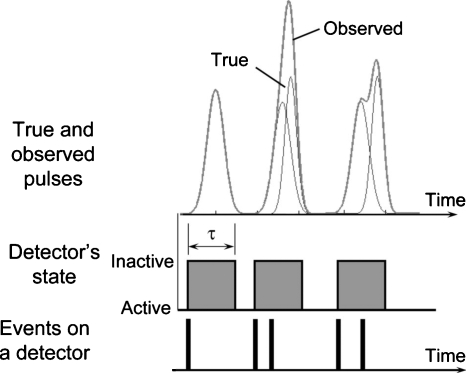
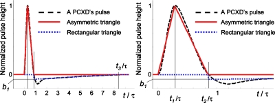
However, due to the limited speed of detectors, quasi-coincident photons are recorded as one count with a higher or lower energy (see Fig. 1). For example, one recent detector has a maximum output count rate of 6 million counts per second (Mcps) per square mm.⁷ [The required operational count rates for clinical x-ray CT detectors varies depending on clinical applications and can be as large as 3–100×10⁶ counts per second per square millimeter (cps∕mm²) for the attenuated beam when the unattenuated count rate incident onto a bowtie filter is 1×10⁹ cps∕mm² measured at 1 m away from the x-ray source.¹²] The operational input count rate of the detector, however, must be below 0.5 Mcps in order to avoid distortion of the recorded spectrum due to pulse pileup effects. With higher count rates, two types of pulse pileup effects are observed: Peak pileup and tail pileup. A typical bipolar pulse shape is shown in Fig. 2. Coincidences during the initial part of pulses are recorded as a single count at a higher energy than the original pulse’s energy (see Fig. 1). This is called peak pulse pileup.¹³ The long tail of the pulse affects the recorded energy of subsequent events; for bipolar-shaped pulses, a peak overlapping the tail of a preceding pulse results in a smaller recorded energy. This is called tail pulse pileup.¹³ Both of these pulse pileup effects distort the recorded spectrum and the amount of distortion will depend on the count rate. Thus, using data from the recorded spectrum in material decomposition process without compensation or correction will produce inaccuracies. Ideally, faster detectors with fewer pulse pileup distortions would be used, but this may be practically impossible. Alternatively, hardware-based pileup rejectors can reduce or eliminate the spectral distortion due to peak pileup; however, the efficiency of such rejectors could be limited (e.g., 50%) for various reasons.^{13, 14, 15, 16} The precision of measurements may be significantly degraded since there are fewer counts without pileup effects. In addition, it is quite challenging to implement pileup rejectors in a PCXD since they would need to operate at very high count rates. Even after attenuation by a bowtie filter and an object, the required operational count rates for clinical x-ray CT systems may be as large as 3–50 Mcps when the incident count rate is 1000 Mcps.¹² Thus, while the detector speed needs to improve, it is also desirable to develop algorithmic methods to compensate for these pulse pileup effects in order to take full advantage of the energy discrimination capabilities of PCXDs. In simulation studies (see Fig. 9 in Sec. 4B), we have found that a significant fraction of recorded counts result from pileup with orders of up to 3, where pileup of order m indicates thatm+1 photons contribute to one recorded count.¹⁴ The key to successful compensation methods is a fast and accurate method to model both pulse pileup effects for realistic (especially bipolar) pulse shapes sufficiently well and to be able to handle pileup orders of up to 3.

Figure 1.

The count rate loss and pulse pileup effects due to quasicoincident photons with nonparalyzable photon counting detectors. When photon counting detectors are in active state, the first photon incident on the detector will put the detector into the detection (inactive) state for a finite period of time called the deadtime (or resolving time) τ. The height of the observed pulse during the deadtime is associated with the photon energy and a count is added to the corresponding energy window. All photons incident on the detector during this state will contribute to form the observed pulse of one count, resulting in lost counts and distorted recorded energy spectrum.

Figure 2.

A bipolar-shaped pulse (dashed black curve) obtained by a PCXD is approximated by two triangles. An asymmetric triangle defined by t₁ and t₂ approximates the positive part of the pulse for peak pileup effect, while a right angle (rectangular) triangle defined by t₂, t₃, and b₁ fits the negative part for tail pileup effect. Two plots are shown in different ranges.

Figure 9.

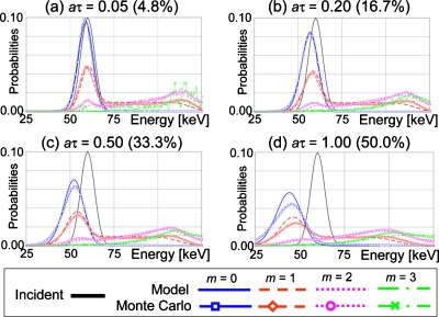
The PDF of the recorded spectra for mth order pileup Pr(E|m), with the quasimonochromatic 60 keV input x-ray spectrum at various relative count rates aτ, obtained using the model and Monte Carlo simulations. Numbers in parentheses are count rate loss ratios, 1−Pr(rec|aτ) (%). Oscillations in Monte Carlo results (e.g., m=3 with aτ=0.05) was due to a limited number of cases (counts).

In previous work, we had developed an analytical pulse pileup model¹⁷ and methods to compensate for pulse pileup effects.^{18, 19} The model, however, used the following three oversimplistic assumptions: (1) The pulse shape was rectangular; (2) the recorded energy was assumed independent of the time interval between coincident photons; and thus (3) the recorded energy was the sum of original energies. These assumptions tend to overestimate the recorded energies as reported by Tennery;²⁰ as a result, we found that the estimated spectrum deviated from the recorded spectrum. Wielopolsk and Gardner¹³ used a parabola or polynomials²¹ to model the pulse shape and to predict the peak pileup effect for first order pileup events (m=1); the parabola model was later extended to second order pileup by Barradas and Reis.¹⁶ However, these models did not account for the tail pileup effect. Johns and Yaffe¹⁵ used a random or periodic pulse generator, with or without a pulse pileup rejector, to estimate the incident count rate and spectrum, but the method will not work without the special pulse generator. Others have used empirical filters to predict peak pileup effects;²² however, the accuracy was limited because of simplifications and the use of empirical kernels. To our best knowledge, there have been no analytical models that satisfy all of the requirements discussed above.

The aim of this study was, thus, to develop a new analytical pulse pileup model which meets all of the requirements discussed above for a typical PCXD. In order to improve accuracy, the model takes into account the following factors: The probability distribution of time intervals between photons, the probability distribution of photon energies, and a more realistic average pulse shape. We performed Monte Carlo (MC) simulations using monochromatic and polychromatic incident spectra to assess the performance of the proposed model.

The structure of this paper is as follows. The analytical model of pulse pileup effects is described in Sec. 2. Section 3 outlines evaluation methods, and results are presented in Sec. 4. In Sec. 5, relevant issues are discussed and the paper is concluded.

ANALYTICAL MODELS OF PULSE PILEUP EFFECTS

The following presents the analytical models. We explain the counting mechanism, a simplified detection mechanism, models of peak pileup, tail pileup, and the recorded spectrum with pulse pileup effects.

Counting (detection) mechanism and two detector models

The detection mechanism for most of PCXDs can be modeled reasonably well by either the nonparalyzable or paralyzable model.¹⁴ When detection mechanisms are realized by electric circuits, most detector systems, even those with a simple pulse height analysis, behave somewhere in between. When the detector is in the active state, the first photon incident on the detector will put the detector into the detection state for a finite period of time called the deadtime (or resolving time) τ. All photons incident on the detector during the deadtime (potentially) contribute to the pulse shape of the recorded count. For nonparalyzable detectors, a new event will not reset the time clock for the deadtime with such photons and the detector will return to the active state after the deadtime τ (Fig. 1). By contrast, in a paralyzable detector, each detected photon resets the time clock and the detector returns to the active state a time τ after an event if, and only if, there is no additional incident photon during the deadtime interval.

Energy discrimination capabilities are often added to PCXDs by the addition of one or more thresholds to the detection chain. For either type of detector, a count is registered in a counter associated with a given threshold if the pulse height exceeds the threshold. Subtracting counts in counters from adjacent energy thresholds, yields the counts in the energy window defined by the two thresholds.

For low true count rates [a⪡1∕τ (the unit of the deadtime τ is seconds per count, when multiple occurrences of deadtime τ over a sufficiently long measurement time period are discussed), where a is the true count rate], the two methods provide identical results.¹⁴ For the sake of simplicity, and since the nonparalyzable detector model fit better with measured count rates in preliminary experiments (not shown), the nonparalyzable detector model was used throughout this study.

Overview of the model

The mean number of recorded photons at energy E with pulse pileup effects, N_PPE(E), can be expressed as the product of three probabilities

$$N_{\text{PPE}}\left(E\right)=\left(\text{True}\text{count}\text{rate}\right)\times \left(\text{Probability}\text{of}\text{events}\text{being}\text{recorded}\right)\times \sum _{m=0}^{\infty }\left[\left(\text{Probability}\text{of}\text{the}m\text{th}\text{order}\text{pulse}\text{pileup}\text{event}\right)\times \left(\text{Probability}\text{of}\text{counts}\text{recorded}\text{at}\text{an}\text{energy}E\text{with}m\text{th}\text{order}\text{pulse}\text{pileup}\right)\right],$$ (1)

$$=a\times \text{Pr}\left(\text{rec}|a\tau \right)\times \sum _{m=0}^{\infty }\text{Pr}\left(m|\text{rec}\right)\text{Pr}\left(E|m\right),$$

$$=a\times \text{Pr}\left(\text{rec}|a\tau \right)\times \text{Pr}\left(E|\text{rec}\right)\left(\because \text{Pr}\left(E|\text{rec}\right)=\sum _{m=0}^{\infty }\text{Pr}\left(m|\text{rec}\right)\text{Pr}\left(E|m\right)\right),$$

where a is the true count rate, τ is the detector deadtime, and Pr(E|rec) is the probability density function (PDF) of the recorded energy E given the events-of-interest being recorded. The first two probabilities for the nonparalyzable model have been discussed in Ref. 14 and are

$$\text{Pr}\left(\text{rec}|a\tau \right)=1∕\left(1+a\tau \right)$$ (2)

and

$$\text{Pr}\left(m|\text{rec}\right)={\left(a\tau \right)}^m\text{exp}\left(-a\tau \right)∕m!.$$ (3)

Equation 3 is the Poisson probability of having m events during time τ, given the mean number of counts aτ. Here we provide a brief explanation for Eq. 2. When the recorded count rate is a_R, the fraction of time that the detector is inactive (dead) is given by a_Rτ. Thus, the rate at which counts are lost during the time period is aa_Rτ, which is also given by a−a_R. Equating these two expressions for the lost count rate, we have a−a_R=aa_Rτ. Solving for a_R and dividing both sides of the equation by a, we get Pr(rec|aτ)=a_R∕a=1∕(1+aτ). The third probability of Eq. 1, Pr(E|m), or the PDF of pulse pileup spectrum for a given pulse pileup order m, will be derived in Sec. 2C.

Probability density function of pulse pileup spectrum

In this subsection, we derive the third probability in Eq. 1: The PDF of the recorded spectrum with a given pulse pileup order m, Pr(E|m). To provide good accuracy, the model takes into account the following factors: The probability of time intervals between photons, the probability of photon energies, and the shape of pulses. Estimating the peak pileup effect, which defines the overall shape of the spectrum, requires better models for all of the above three factors than estimating the tail pileup effect. Modeling the tail pileup effect, which simply offsets the energy spectrum resulting from peak pileup effect, requires a less accurate model.

Pulse shape of DxRay’s PCXD

Figure 2 shows the scaled bipolar pulse shape of the DxRay PCXD (Ref. ⁷) modeled in this work, which was obtained using a high speed oscilloscope. We assume that the pulse shape scales in proportion to energy in the vertical direction but is independent of energy in the horizontal (time) direction. That is, the time duration is independent of photon energy. We modeled this bipolar pulse shape by two triangle functions and treated them separately. An asymmetric triangle function was used for the positive lobe on the time interval [0,t₂], with the maximum occurring at t₁. This allowed us to model the peak pileup effect accurately and efficiently. The parameters t₁ and t₂ were estimated using least-squares fitting. A right angle (rectangular) triangle function fitted to the negative part on the time interval [t₂,t₃] was used to model tail pileup effect. The parameters t₃ and b₂ were estimated using least-squares fitting. In our study, the values were found as follows while setting a deadtime τ slightly larger than t₂: t₁=0.284×τ, t₂=0.850×τ,t₃=8.253×τ, and b₂=−0.0635, respectively. The ratio of t₂∕τ was determined empirically; an optimal value for each detector may vary, although it may be close to, but less than, 1. Note that there was no inconsistency in these parameter values in this study because we used the same detector deadtime τ for both Monte Carlo simulations and our models.

Event recording model

Rather than estimating the number of counts above a specific threshold, we have chosen to calculate the energy spectrum. This is somewhat of an approximation to the actual counting mechanism and was done in order to facilitate efficient calculation of the effects of peak and tail pileup. We modeled the detection process as follows. We assume that an event arrives at t=0 with the detector in the active state and thus triggers the detection process. The detection state lasts until t=τ. Pulses from subsequent photons incident during this interval are summed to form a single observed pulse. The maximum height of the observed pulse between t=0 and τ is recorded. After the time t=τ, the detector returns to the active state and the remaining pulse shape is carried over and summed with any subsequent pulses that occur before time t₃. This model allows us to efficiently calculate the recorded spectrum with very fine energy threshold spacing, e.g., a 1 keV increment. An alternate approach would be to have a finite number of energy thresholds and model the exact detection scheme of a specific detection circuit. This approach would limit the number of energy thresholds, since a large number of energy thresholds would increase computational costs.

First order peak pileup effect

We start with the pulse pileup order m=1 (i.e., when two photons are involved with a recorded count). The PDF (distribution function) for time intervals between adjacent random events I₁(t) is¹⁴

$$I_1\left(t\right)dt=a\text{\hspace{0.17em}exp}\left(-at\right)dt.$$ (4)

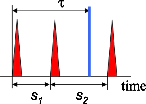
Let s_i be the time interval between the (i−1)th event and the ith event. For m=1 pileup to occur, the first event must occur within a time τ from the zeroth event (s₁≤τ) and the second event must be outside τ (s₁+s₂>τ) (see Fig. 3). The distribution function I^(m=1)(s₁) for m=1 pileup events where the time between the two piled-up events is s₁ can then be obtained by

$$I^{\left(m=1\right)}\left(s_1\right)d{s}_1=I_1\left(s_1\right)\left[{\int }_{\tau -s_1}^{\infty }{I}_1\left(s_2\right)d{s}_2\right]d{s}_1=a\text{\hspace{0.17em}exp}\left(-a{s}_1\right){\int }_{\tau -s_1}^{\infty }a\text{\hspace{0.17em}exp}\left(-a{s}_2\right)d{s}_{2}d{s}_1,$$ (5)

$$=a\text{\hspace{0.17em}exp}\left(-a\tau \right)d{s}_1=\text{const}\text{.}\times d{s}_1.$$

Since ${\int }_0^{\tau }d\text{\hspace{0.17em}Pr}\left(s_1|m=1\right)d{s}_1=1$ and I^(m=1)(s₁)ds₁=0 for s₁<0 or s₁>τ, the differential probability of time intervals given pulse pileup order 1 is

$$d\text{\hspace{0.17em}Pr}\left(s_1|m=1\right)=\frac{I^{\left(m=1\right)}\left(s_1\right)d{s}_1}{{\int }_0^{\tau }{I}^{\left(m=1\right)}\left(s^{\prime }\right)d{s}^{\prime }}=\frac{\text{const}\text{.}\times d{s}_1}{\text{const}\text{.}\times \tau }=1∕\tau d{s}_1.$$ (6)

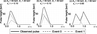
Now we consider the recorded energy as a function of the energies of the two photons E₀ and E₁, and the time interval between them (s₁). For a simple triangular pulse shape, the recorded energy E_R is equal to the maximum of the summed triangles and must be found at one of the peaks of the two pulses or at t=τ (see Fig. 4) because the derivatives of observed pulses are piecewise constant. The value of E_R can be expressed analytically, as shown in Appendix B.

Figure 3.

Time intervals s₁ and s₂ and detector deadtime τ.

Figure 4.

Pictorial descriptions of an observed pulse with given energies and a time interval between two events. The recorded energy E_R(s₁;E₀,E₁) is the maximum energy between t=0 and τ. (a) E₀=50 keV, E₁=20 keV, and s₁∕τ=0.10; (b) E₀=50 keV, E₁=40 keV, and s₁∕τ=0.10; and (c) E₀=50 keV, E₁=60 keV, and s₁∕τ=0.65.

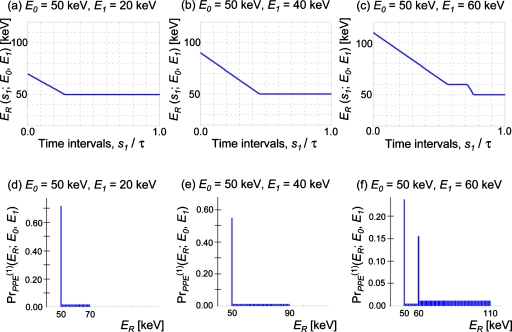
Using the differential probability of s₁ given m=1 [Eq. 6], we obtain the PDF of the recorded energy E, given the incident energies E₀ and E₁. A general formula, shown in Eq. 7, was used to obtain the specific results shown in Appendix C and Fig. 5.

$${\text{Pr}}_{\text{PPE}}^{\left(1\right)}\left(E;E_0,E_1\right)=\int d\text{\hspace{0.17em}Pr}\left(s_1|m=1\right){|}_{E_R\left(s_1;E_0,E_1\right)=E}d{E}_R.$$ (7)

Using the incident spectrum S₀(E), the PDF of the recorded spectrum with first order peak pulse pileup can be calculated using

$${\text{Pr}}_{\text{peak}}\left(E|m=1\right)={\int }_0^{\infty }{\int }_0^{\infty }{\text{Pr}}_{\text{PPE}}^{\left(1\right)}\left(E;E_0,E_1\right)S_0\left(E_0\right)S_0\left(E_1\right)d{E}_{0}d{E}_1.$$ (8)

Figure 5.

[(a)–(c)] The recorded energies E_R(s₁;E₀,E₁) given various time intervals s₁ and the incident energies E₀ and E₁. [(d)–(f)] The PDFs of the recorded energies E_R given the incident energies E₀ and E₁ for pileup order 1.

Higher order pileup effects

For m=2 to occur, both the first and the second events must occur within a time τ from the zeroth event and the third event must be outside τ. The distribution function for time intervals with m=2, I^(m=2)(s₁), can then be obtained by

$$I^{\left(m=2\right)}\left(s_1\right)d{s}_1=I_1\left(s_1\right)\left[{\int }_0^{\tau -s_1}{I}_1\left(s_2\right)\left\{{\int }_{\tau -s_1-s_2}^{\infty }{I}_1\left(s_3\right)d{s}_3\right\}d{s}_2\right]d{s}_1=a^2{e}^{-a\tau }\left(\tau -s_1\right)d{s}_1.$$ (9)

Thus, for ${\int }_0^{\tau }d\text{\hspace{0.17em}Pr}\left(s_1|m=2\right)d{s}_1=1$, the differential probability of time intervals is

$$d\text{\hspace{0.17em}Pr}\left(s_1|m=2\right)=2∕{\tau }^2\times \left(\tau -s_1\right)d{s}_1.$$ (10)

Photons are independent and identically distributed, thus, d Pr(s₂|m=2)=d Pr(s₁|m=2).

With a given set of three energies, E₀, E₁, and E₂, we wish to obtain the PDF of recorded energy ${\text{Pr}}_{\text{PPE}}^{\left(2\right)}\left(E_R;E_0,E_1,E_2\right)$, and use a triple integration over energies similar to Eq. 8. However, analytical expressions for recorded energiesE_R⁽²⁾(s₁,s₂;E₀,E₁,E₂), used to calculate ${\text{Pr}}_{\text{PPE}}^{\left(2\right)}$, are already complex. The expressions become even more complex as the pileup order m increases. Thus, we approximate the mth order pulse pileup for m>1 as follows.

We recursively calculate the PDF of the recorded energy

$${\text{Pr}}_{\text{peak}}\left(E|m>1\right)={\int }_0^{\infty }{\int }_0^{\infty }{\text{Pr}}_{\text{PPE}}^{\left(1\right)}\left(E;E_{m-1},E_1\right)\text{Pr}\left(E_{m-1}|m-1\right)S_0\left(E_1\right)d{E}_{m-1}d{E}_1,$$ (11)

while the differential probability function of time intervals for the corresponding (correct) pileup order m is used as

$${\text{Pr}}_{\text{PPE}}^{\left(1\right)}\left(E;E_{m-1},E_1\right)=\int d\text{\hspace{0.17em}Pr}\left(s_1|m\right){|}_{E_R\left(s_1;E_{m-1},E_1\right)=E}dE$$ (12)

and

$$d\text{\hspace{0.17em}Pr}\left(s_1|m\right)=m∕{\tau }^m\times {\left(\tau -s_1\right)}^{m-1}d{s}_1.$$ (13)

Here, we approximate higher order pileup as follows. A virtual photon is incident on the detector at t=0 that carries the same energy as the maximum energy of the observed pulse from the first m photons [which would be the recorded energy in the absence of pileup for photon (m+1)]. The time intervals between the virtual photon and the (m+1)th photon are distributed according to the differential probability density for the corresponding pileup order m [Eq. 13]. The recorded energy is then calculated by the scheme developed for the case of m=1 using the energies of the virtual and the (m+1)th photon and the probability of time intervals for mth order pileup. This simplification allows us to efficiently and easily handle higher order pileup, since all we have to know for each order m is d Pr(s₁|m). The accuracy of this scheme will be evaluated using Monte Carlo simulations.

Tail pileup effect

Previous events that occurred within a time t₃ from the zeroth event in the events-of-interest (i.e., −t₃<t) will result in the tail pileup effects, decreasing the recorded energy of the events-of-interest. Because the time duration of the tail (t₃) is long, and thus its effect is limited to a (negative) bias to the recorded energy, the tail pileup effect is modeled differently from the peak pileup effect. We acknowledge that the model does not consider a possibility of a part of the peak from the previous events being carried over to the subsequent event. The effect of the absence will be evaluated using Monte Carlo simulations.

The mean counts during time duration t₃ is at₃, where a is the true count rate. The Poisson probability of n photons is then

$$\text{Pr}\left(n|a{t}_3\right)={\left(a{t}_3\right)}^n{e}^{-a\tau }∕n!.$$ (14)

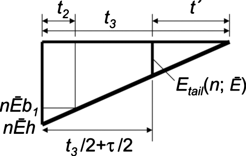
We simply assume that n events are uniformly distributed and centered at t=−t₃∕2, and that all of the n events carry the mean energy $\overline{E}$ of the incident spectrum S₀(E). These n photons will provide a negative offset for the peak pulse height in the events-of-interest measured at t=τ∕2 of an amount $E_{\text{tail}}\left(n;\overline{E}\right)$ (<0), which can be calculated as follows. From the geometrical relation shown in Fig. 6, we have

$$E_{\text{tail}}\left(n;\overline{E}\right)∕t^{\prime }=n\overline{E}h∕t_3,$$ (15)

where h (<0) is the y-intercept when the negative right angle triangle shown in Fig. 2 is extended to t=0, and can be calculated by

$$h=b_1\times t_3∕\left(t_3-t_2\right).$$ (16)

Using Eqs. 15, 16 and

$$t^{\prime }=t_3-\left(\frac{t_3}{2}+\frac{\tau }{2}\right)=\left(t_3-\tau \right)∕2,$$ (17)

the negative offset, $E_{\text{tail}}\left(n;\overline{E}\right)$, can be calculated as

$$E_{\text{tail}}\left(n;\overline{E}\right)=\frac{n\overline{E}{b}_1}{2}\times \frac{t_3-\tau }{t_3-t_2}\le 0.$$ (18)

With a given $\overline{E}$,

$${\text{Pr}}_{\text{tail}}\left(E_{\text{tail}}\right)=\text{Pr}\left(E_{\text{tail}}\left(n;\overline{E}\right)|a{t}_3\right)=\text{Pr}\left(n|a{t}_3\right).$$ (19)

Figure 6.

Tail pileup effect: The bias $E_{\text{tail}}\left(n;\overline{E}\right)$ (<0) is added to the measured energy of the subsequent events-of-interest.

Recorded spectrum with pileup effects

By taking into account the energy shift due to the tail pileup effect on the recorded spectrum resulting from modeling the peak pileup effect, we obtain the PDF of recorded spectrum with pulse pileup order m

$$\text{Pr}\left(E|m\right)={\int }_{-\infty }^{\infty }{\text{Pr}}_{\text{peak}}\left(E-E_{\text{tail}}|m\right){\text{Pr}}_{\text{tail}}\left(E_{\text{tail}}\right)d{E}_{\text{tail}}.$$ (20)

Notice that this model requires relatively modest amounts of information about the PCXD. The information needed includes the pulse shape (defined by the parameters b, t₁, t₂, and t₃) and the deadtime τ. Given the incident count rate and energy spectrum, the model then predicts the recorded spectrum.

EVALUATION METHODS

We first evaluated the accuracy of approximating the actual pulse shapes by the two triangular functions. We then used Monte Carlo simulations to evaluate the accuracy of energy spectra estimated using the proposed pulse pileup model. In the evaluation of energy spectra, pileup orders (values of m) of up to 6 were used, which covers more than 99.9% of recorded events.

Recorded spectrum with peak pileup only

First, we evaluated how well the recorded energiesE_R⁽¹⁾(s₁;E₀,E₁) were modeled by the proposed triangular function compared to those estimated using the actual shape of the DxRay pulse for various combinations of recorded energies and time between pulses. A numerical array containing the DxRay’s pulse shape (Fig. 2) was scaled by each of the input energies of E₀, E₁ to give the two input pulses. They were then added to form an observed pulse with various offsets, corresponding to various time intervals s₁ between the pulses. The maximum height of the observed pulse between t=0 and τ was recorded and compared to the recorded energy calculated by the model E_R⁽¹⁾(s₁;E₀,E₁).

The photon energy of either E₀ or E₁ was varied from 0 to 100 keV with a 1 keV increment, while the other was fixed at 50 keV, and s₁∕τ was varied between 0 and 1 with an increment of 0.01. Differences in the recorded energy from the real pulse shape and triangular model were quantified by the root mean square difference (RMSD) and the coefficients of variation (COV). Formulas for these are given below.

Monte Carlo simulation program

We used a Monte Carlo simulation program developed in our laboratory, which stochastically generates photons using the distribution function for intervals between adjacent random events, I₁(t)=a exp(−at)dt.¹⁴ The energy of each photon was randomly sampled using the PDF of the incident spectrum. The scheme discussed in Sec. 3A was used to obtain the observed pulse shape numerically, and the recorded energy and the pulse pileup order m were stored. The tail of the observed pulse shape was added to the pulse shape of the subsequent events-of-interest. After a predetermined number of photons were generated, the recorded energies of events-of-interest were sorted and binned with a width of 1 keV.

We verified the Monte Carlo program with the following measurements: The recorded count rate curve agreed with the theoretical prediction [Eq. 2] (see Sec. 4B); the probabilities of mth order pileup agreed to the theoretical prediction [Eq. 3] (see Sec. 4B); the PDF of the recorded spectrum with a very fast detector (aτ=0.001) was identical to the PDF of the incident spectrum; the PDF of the recorded spectrum was distorted toward higher energy with higher count rates when a monopolar pulse shape (i.e., a pulse shape with no negative lobe) was used (not shown); and the PDF of the recorded spectrum was distorted toward lower energy with higher count rates when a bipolar pulse shape was used, as will be seen in the results of this study (see Secs. 4B, 4C).

Monte Carlo simulation with monochromatic spectrum

We first performed a Monte Carlo simulation using a quasimonochromatic spectrum. Modeling pileup effects for a sharply peaked, monochromatic spectrum is more challenging than for a broad, polychromatic spectrum, since the former shows the effects of both peak and tail pileup more clearly than the latter. The quasimonochromatic spectrum was a normal distribution centered at 60 keV with a full-width-at-half-maximum of 10 keV. The detector deadtime τ was fixed at 100 ns. We investigated count rates a of 0.1, 0.2, 0.5, 1, 2, 5, 10, or 20 Mcps, which corresponded to aτ of 0.01, 0.02, 0.05, 0.10, 0.20, 0.50, 1.00, and 2.00, respectively. We simulated a total of 10⁷ photons for each count rate setting.

Results were compared to the proposed model. First, the probability of counts being recorded Pr(rec|aτ) was compared to the model [Eq. 2]; the RMSD and the COV were calculated. Second, the probability of mth order pileup events given the events-of-interest being recorded Pr(m|rec) were compared to the model [Eq. 3]; the RMSD and the COV were calculated. Third, the PDF of the recorded spectrum for mth order pileup Pr(E|m) was qualitatively compared to the PDF obtained by the model [Eq. 20]. Fourth, the PDFs of the recorded spectra, Pr(E|rec), were compared both qualitatively and quantitatively to those predicted by the model for each count rate setting. The following four descriptors of the PDF, the mean (μ), the standard deviation (σ), the skewness, and the kurtosis of the PDF (see Appendix A) were calculated, as well as the RMSD and the COV between the PDF obtained with Monte Carlo simulation and with the model. Energy bins with probabilities less than 0.0005 were excluded from the calculations of RMSD and COV.

Monte Carlo simulation with polychromatic x ray

We performed a Monte Carlo simulation using a polychromatic x-ray beam containing an transmission K-edge. A 90 kVp spectrum was obtained using the IPEM program²³ with a tungsten anode and an anode angle of 7°. The spectrum was then attenuated by 1.0 mm of aluminum, 1.2 mm of titanium, and 0.5 mm of gadolinium. The other conditions were the same as in Sec. 3C, and the results were assessed in the same way.

Quantitative measures of agreement

To quantitatively assess the degree of agreement we calculated the RMSD and COV using the formulas

$$\text{RMSD}=\sqrt{\sum _{i=1}^N{\left(x_{i,\text{Ref}}-x_{i,\text{model}}\right)}^2∕N},$$ (21)

$$\text{COV}=\text{RMSD}∕\left(\sum _{i=1}^N{x}_{i,\text{Ref}}∕N\right)\times 100\left[\mathrm{\%}\right],$$ (22)

where x_i,Ref is the reference value (obtained, e.g., using the true pulse shape or Monte Carlo simulation) at sampling point, i, x_i,model is the value at i predicted by the analytical model, and N is the number of sampling points.

EVALUATION RESULTS

Recorded spectrum with peak pileup only

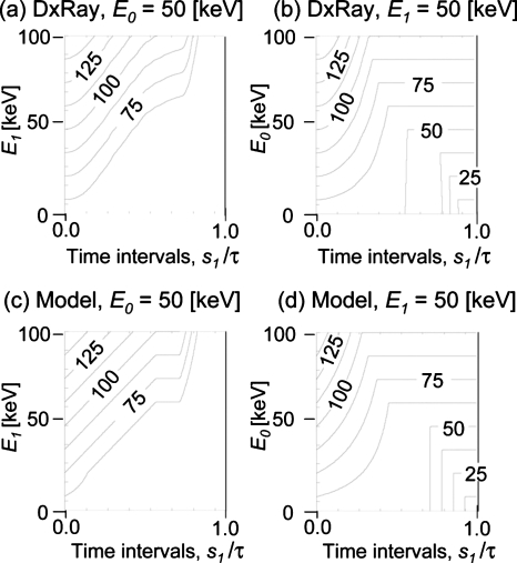
Figure 7 shows contour maps of E_R⁽¹⁾ under various conditions. The agreement was excellent in each case: RSMD and COV were 2.29 keV and 3.21% between Figs. 7a, 7c, respectively, and 3.29 keV and 4.60% between Figs. 7b, 7d, respectively. The asymmetric triangle fits the positive part of the pulse reasonably well (see Fig. 2); thus, only relatively minor effects due to deviations in the pulse shape were observed. The right angle triangle fits the negative part of the pulse with a long duration (t₂<t<∼8.3τ); however, a relatively large deviation exists in the dip at the initial part of the negative pulse for t₂<t<1.8τ (see Fig. 2). The effect of this deviation will appear only if position of the maximum occurs within this dip. The results indicated that this effect was small.

Figure 7.

Contour maps of the recorded energy with first order pulse pileup (m=1) under various conditions when the observed pulse height is 0 at t=0.

Monte Carlo simulation with monochromatic spectrum

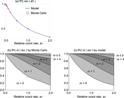
Figure 8a shows the plots of the probability of counts being recorded, Pr(rec|aτ), at various count rates, obtained by the Monte Carlo simulation and by the model [Eq. 2]. The RMSD and COV were 1.30×10⁻³ and 0.17%, respectively, demonstrating an excellent agreement. Figures 8b, 8c show area plots of the probabilities of mth order pileup given the events-of-interest being recorded at various count rates, obtained by the Monte Carlo simulation and by the model [Eq. 3]. The RMSD and COV were 3.10×10⁻⁴ and 0.19%, respectively, again demonstrating 20 excellent agreement. Note that we have targeted using PCXDs under conditions where 0.05≤aτ≤1.0 (corresponding to a deadtime loss of 5%–50%) for PCXD-based CT imaging using this pulse pileup model. Figure 8 confirmed that pulse pileup orders of up to 3 (0≤m≤3) are then necessary and sufficient.

Figure 8.

(a) A plot of the probability of events being counted Pr(rec|aτ), obtained by the model and by Monte Carlo simulations. [(b) and (c)] Area plots of the probabilities of mth order pileup given the events-of-interest being counted Pr(m|rec), obtained by (b) Monte Carlo simulations and by (c) the model.

Figure 9 shows the PDFs of the recorded spectrum obtained with the quasimonochromatic incident spectrum of 60 keV, given the mth order pileup Pr(E|m) [Eq. 20] at count rates of 0.5, 2, 5, and 10 Mcps (with aτ of 0.05, 0.20, 0.50, and 1.00). Probabilities for recorded energies above 60 keV with m>0 increased compared to the incident spectrum, demonstrating the effect of the peak pileup; spectra predicted by the model showed excellent agreement with those generated by Monte Carlo simulations up to third order pileup (m=3), although the spectra obtained by Monte Carlo simulations seem to be slightly broader, especially for aτ=1.00 or m=0. The deviation might be because the model does not take into account the possibility of part of the peak from the previous events being carried over to the subsequent event, as discussed in Sec. 3. The recorded spectra for the higher count rates exhibited decreased energies, especially those of m=0, due to the tail pileup effect, and the model successfully predicted this count rate-dependent phenomenon.

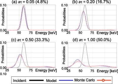
Figure 10 shows the PDFs of the total recorded spectra at various incident count rates; the four cases correspond to those shown in Fig. 9. The spectra calculated with the model were in an excellent agreement with those obtained with Monte Carlo simulations in terms of the peak energies and the tails of the spectra.

Figure 10.

The PDF of the total recorded spectra Pr(E), the quasimonochromatic 60 keV input x-ray spectrum at various relative count rates aτ, obtained by the model and Monte Carlo simulations. Numbers in parentheses are count rate loss ratio 1−Pr(rec|aτ) (%).

Tables 1, 2 summarize the results of the quantitative analyses. All of the four descriptors of the PDFs shown in Table 1 were in an excellent agreement for aτ≤1.0, confirming the subjective assessment of the recorded spectra (Figs. 910). The RMSD values were consistently small and COV values were less than 18.4 for the targeted range of aτ≤0.5 (Table 2).

Table 1.

Four statistical descriptors of recorded spectrum with quasimonochromatic x-ray spectrum of 60 keV obtained by MC simulations and the model.

		Relative count rates aτ (count rate loss ratio)
		0.01 (1.0%)	0.02 (2.0%)	0.05 (4.8%)	0.10 (9.1%)	0.20 (16.7%)	0.50 (33.3%)	1.00 (50.0%)	2.00 (66.7%)
Mean (keV)	MC	59.2	59.2	59.4	59.7	60.4	62.9	68.4	83.5
	Model	59.7	59.7	59.8	59.9	60.3	62.1	66.2	75.3
	% errors	1.0	0.9	0.6	0.3	0.1	1.3	3.2	9.8
St. dev. (keV)	MC	4.9	5.8	7.9	10.6	14.7	23.5	34.0	48.5
	Model	4.8	5.6	7.3	9.7	13.5	22.3	33.1	45.0
	% errors	2.1	4.6	7.3	8.2	7.8	5.0	2.7	7.3
Skewness	MC	3.7	4.5	4.5	3.9	3.0	1.9	1.3	0.8
	Model	2.8	3.8	4.3	4.0	3.3	2.2	1.5	0.7
	% errors	23.3	16.2	5.2	2.3	9.2	16.8	14.7	9.2
Kurtosis	MC	42.5	44.2	33.3	22.3	13.7	7.2	4.8	3.4
	Model	32.1	37.3	33.2	24.8	16.7	8.9	5.1	2.9
	% errors	24.4	15.6	0.3	11.0	21.4	24.6	7.1	12.7

Table 2.

RMSD and COV of recorded spectrum with quasimonochromatic x-ray spectrum of 60 keV obtained by the model.

	Relative count rates aτ (count rate loss ratio)
	0.01 (1.0%)	0.02 (2.0%)	0.05 (4.8%)	0.10 (9.1%)	0.20 (16.7%)	0.50 (33.3%)	1.00 (50.0%)	2.00 (66.7%)
RMSD (×10−3)	6.19	5.43	3.26	1.51	1.14	1.73	1.86	1.26
COV (%)	16.2	14.8	13.6	12.3	10.0	18.4	29.1	27.4

Monte Carlo simulation with polychromatic x ray

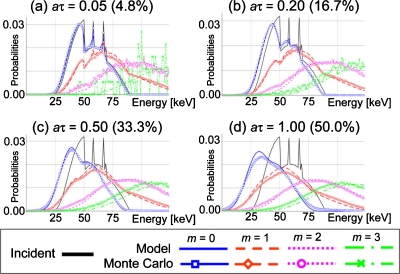
Figure 11 shows the PDFs of the recorded spectra obtained with the 90 kVp polychromatic incident spectrum for mth order pileup Pr(E|m) [Eq. 20] at count rates of 0.5, 2, 5, and 10 Mcps (aτ of 0.05, 0.20, 0.50, and 1.00). The spectra predicted by the model agreed very well with those from Monte Carlo simulations. The spectrum shape near the gadolinium K-edge (50 keV) changed as the count rates increased, which was accurately predicted by the model; the sharpness of the K-edge was reduced and it was distorted toward lower energies. The PDFs for m=0 were distorted toward lower energies as the count rates were increased. The shape and extent of spectra above 90 keV were also in good agreement.

Figure 11.

The PDFs of the recorded spectrum for mth order pileup Pr(E|m), with 90 kVp polychromatic input x-ray spectrum at various relative count rates aτ, obtained using the model and Monte Carlo simulations. Numbers in parentheses are count rate loss ratio 1−Pr(rec|aτ) (%). Oscillations in Monte Carlo results (e.g., m=3 with aτ=0.05) were due to a limited number of cases (counts).

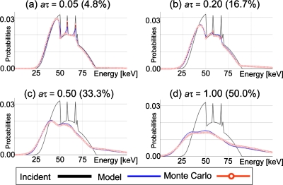
Figure 12 shows the PDFs of the total recorded spectra at various count rates; the four cases correspond to those shown in Fig. 11. The spectra calculated using the model were in an excellent agreement with those from Monte Carlo simulations in terms of the peak energies, the sharpness and height of gadolinium K-edge, and the tails of the spectra.

Figure 12.

The PDFs of the final recorded spectra Pr(E), with 90 kVp polychromatic x-ray at various relative count rates aτ, obtained using the model and Monte Carlo simulations. Numbers in parentheses are count rate loss ratios, 1−Pr(rec|aτ) (%).

Tables 3, 4 summarize the results of the quantitative analyses. All of the four descriptors of the PDFs shown in Table 3 were in an excellent agreement for all of aτ values tested, confirming the subjective assessment of the recorded spectra (Figs. 1112). The RMSD values were consistently small and COV values were equal to or less than 10% for the targeted range of aτ≤1.0 (Table 4).

Table 3.

Four statistical descriptors of recorded spectrum with polychromatic x-ray spectrum with 90 kVp obtained by MC simulations and the model.

		Relative count rates aτ (count rate loss ratio)
		0.01 (1.0%)	0.02 (2.0%)	0.05 (4.8%)	0.10 (9.1%)	0.20 (16.7%)	0.50 (33.3%)	1.00 (50.0%)	2.00 (66.7%)
Mean (keV)	MC	54.3	54.4	54.6	55.0	55.8	58.4	63.9	79.2
	Model	55.0	55.0	55.1	55.3	55.9	57.9	62.9	71.9
	% errors	1.2	1.1	0.9	0.6	0.2	0.8	2.5	9.2
St. dev. (keV)	MC	14.1	14.4	15.2	16.6	19.2	25.8	34.5	47.1
	Model	14.0	14.3	15.0	16.2	18.5	25.0	34.0	44.0
	% errors	0.2	0.6	1.7	2.8	3.7	3.1	1.5	6.4
Skewness	MC	0.4	0.5	0.8	1.1	1.3	1.3	1.1	0.8
	Model	0.4	0.4	0.7	0.9	1.3	1.5	1.2	0.7
	% errors	9.4	12.6	14.4	10.4	2.5	10.3	10.4	10.8
Kurtosis	MC	2.9	3.4	4.7	5.7	6.4	5.8	4.6	3.5
	Model	2.7	3.1	4.1	5.3	6.5	6.5	4.8	3.1
	% errors	6.1	9.1	11.2	6.6	2.5	12.9	4.5	11.0

Table 4.

RMSD and COV of recorded spectrum with polychromatic x-ray spectrum with 90 kVp obtained by the model.

	Relative count rates aτ (count rate loss ratio)
	0.01 (1.0%)	0.02 (2.0%)	0.05 (4.8%)	0.10 (9.1%)	0.20 (16.7%)	0.50 (33.3%)	1.00 (50.0%)	2.00 (66.7%)
RMSD (×10−3)	1.53	1.41	1.16	0.76	0.49	0.43	0.61	0.78
COV (%)	9.8	9.2	7.6	7.0	5.3	5.7	10.0	16.2

DISCUSSION AND CONCLUSIONS

We have developed an analytical pileup model of both peak and tail pileup effects for nonparalyzable detectors. The model takes into account the following factors while using the detector deadtime τ as a parameter: The bipolar shape of the pulse, the distribution function of time intervals between random events, and the PDF of photon energies. The model was in excellent agreement with Monte Carlo simulations in terms of the recorded spectrum including pulse pileup effects over a large range of count rates; the COV was equal to or less than 10% with a deadtime loss of up to 50% with a polychromatic x-ray spectrum.

We aimed to develop a pulse pileup model which is accurate and efficient. It has been shown in this study, both qualitatively and quantitatively, that the accuracy of the proposed model is relatively good. The efficiency of the model, however, has not been evaluated. There is no doubt that analytical models including ours are much more efficient than Monte Carlo simulations. Further we believe our model, which uses triangles, is more efficient than others which use other more complex analytical pulse shapes, e.g., a parabola,^{13, 16, 21} because the probability of the recorded energy ${\text{Pr}}_{\text{PPE}}^{\left(1\right)}\left(E;E_0,E_1\right)$ can be calculated in a much simpler fashion for triangles (see Secs. 2C3, 2C4) than for parabolas.^{13, 16, 21} Our current implementation of this algorithm was not optimized for the computational efficiency; thus data on the current computational cost would not be very meaningful.

We acknowledge that statistical tests such as the Kolmogorov–Smirnov test could be employed to evaluate the so called goodness-of-fit of the model. We did not incorporate such tests in this study for the following two reasons. First, the proposed model clearly produces approximations to the true spectrum, and we wanted to evaluate the degree of fit of our model as a function of count rates. Statistical tests, on the other hand, provide a rather binary answer to a null hypothesis: Either the two distributions are the same or they are not. The probability, or a P value, describes the certainty of the binary decision, not the goodness of fit. Second, such tests are used to decide if the null hypothesis can be rejected. In our case, however, the PDFs of recorded spectrum obtained using Monte Carlo simulations were, in fact, different distributions from those obtained using the model. Thus, these tests should always reject the null hypothesis if a large enough number of samples (photons) were used in Monte Carlo simulations. Therefore, we chose RMSD and COV, which provide a continuous value to indicate the quality of the fit.

There is some work that remains. The proposed pulse pileup model is based on a nonparalyzable detection model. A pulse pileup model based on a paralyzable detection model may be desired for some detectors. While the first two probabilities of Eq. 1 are known,¹⁴ the third probability Pr(E|m) needs to be derived. We shall leave the derivation to future studies. Note, however, that both the nonparalyzable and paralyzable detection models behave very similarly if aτ is small.¹⁴ The nonparalyzable detection model may be sufficient, even for paralyzable detectors, in the presence of statistical variations and other factors such as charge sharing that would also influence the recorded spectrum.

An actual PCXD was not used for the evaluation due to the following reasons. First, there are various other factors that would also influence the recorded spectrum (e.g., charge sharing, shift-variant finite energy resolutions, and escape peaks or K-shell photoelectron escape x ray), and thus, one cannot evaluate pileup effects in isolation. Second, we had no access to the ground truth such as the incident count rate, the incident spectrum, detector deadtime, etc. Third, it is not easy to control conditions including the above-mentioned ground truth. Finally, there always exist detector specific issues related to, e.g., pulse shaping circuits, energy responses, energy thresholds (comparators), deadtime measurements, etc. Thus we decided to use Monte Carlo simulations, which allowed us to focus on the pulse pileup effects. A comparison with a real PCXD (Ref. ⁷) is an ongoing research project and beyond the scope of this study, as it requires a series of careful calibrations and determinations of parameters such as the detector deadtime. We shall present the results when they become ready.

We believe that the methodology presented in this paper can be applicable to different detectors with various pulse shapes. The asymmetric triangle function will be used to model the initial part of the pulse and the right angle triangle will be used to model the tail of the pulse. A positive tail for a monopolar pulse can also be modeled by vertically flipping the right angle triangle function.

A method to combine the proposed pulse pileup model with hardware-based pileup rejection circuits or anticharge sharing circuits (e.g., 2×2 pixel summing with coincident detections as used in the Medipix3 detector^{24, 25, 26}) may be of practical interest, but is outside the scope of this study. Some pileup rejectors do accept as many as 50% of the pulse pileup events.¹⁵ The mechanism of rejection∕acceptance must then be modeled and integrated into the pulse pileup model. A charge generated by one photon near the boundary of detector pixels may be shared among adjacent pixels and recorded as lower energies. The anticharge sharing circuit in the Medipix3 detector detects and sums coincident events in adjacent 2×2 pixels to recover the original photon energy. At high count rates, however, such coincident events may actually be due to independent photons. Pulse pileup effects with such detectors, thus, are more complex and may need more sophisticated models.

The proposed pileup model allows us to calculate an expected recorded spectrum from an incident spectrum. Often, however, the incident spectrum is not known. As we did with the previous pileup model,^{18, 19} we plan to integrate the pileup model as a part of the image reconstruction process, that is, as a part of the forward imaging process modeling to compensate for the limited speed of the detector, and to iteratively estimate either the imaged object or the line integrals¹² using, e.g., a maximum likelihood approach.¹¹ Such a compensation method would enable x-ray computed tomography imaging using even the limited speed of multiwindow photon counting detectors currently available.¹²

APPENDIX A: FOUR DESCRIPTORS OF A PROBABILITY DENSITY FUNCTION

The following four descriptors of a PDF, the mean (μ), the standard deviation (σ), the skewness (μ₃∕σ³), and the kurtosis (μ₄∕σ⁴) of the PDF, were calculated as follows:

$$\mu =E\left[X\right]=\int x\text{PDF}\left(x\right)dx,$$ (A1)

$$\sigma =\sqrt{E\left[{\left(X-\mu \right)}^2\right]}=\sqrt{\int {\left(x-\mu \right)}^2\text{PDF}\left(x\right)dx},$$ (A2)

$$\frac{{\mu }_3}{{\sigma }^3}=\frac{E\left[{\left(X-\mu \right)}^3\right]}{{\sigma }^3}=\frac{\int {\left(x-\mu \right)}^3\text{PDF}\left(x\right)dx}{{\sigma }^3},$$ (A3)

$$\frac{{\mu }_4}{{\sigma }^4}=\frac{E\left[{\left(X-\mu \right)}^4\right]}{{\sigma }^4}=\frac{\int {\left(x-\mu \right)}^4\text{PDF}\left(x\right)dx}{{\sigma }^4},$$ (A4)

where X is a random variable with probability density function PDF(x), the operator E[ ] denotes the average or expected value of X, and μ₃ and μ₄ are the third and fourth standardized moment of a random variable X about the mean, respectively.

APPENDIX B: ANALYTICAL EXPRESSIONS OF THE RECORDED E_R

The value of the recorded energy E_R is expressed analytically as a function of the energies of the two photons E₀ and E₁ as follows:

• (i)
  If (t₂−t₁)∕t₁×E₁≤E₀ [see Figs. 4a, 5a],

  $$E_R\left(s_1;E_0,E_1\right)=\{\begin{array}{ll}{E}_0+\left(1-s_1∕t_1\right)E_1\hfill & \left(0\le s_1\le t_1\right)\hfill \\ E_0\hfill & \left(t_1<s_1\right)\hfill \end{array}\phantom{\}}.$$ (B1)
  (ii) If E₁≤E₀<(t₂−t₁)∕t₁×E₁ [see Figs. 4b, 5b],

  $$E_R\left(s_1;E_0,E_1\right)=\{\begin{array}{ll}\left(1-\frac{s_1}{t_2-t_1}\right)E_0+E_1\hfill & \left(0\le s_1\le E_1∕E_0\times \left(t_2-t_1\right)\right)\hfill \\ E_0\hfill & \left(E_1∕E_0\times \left(t_2-t_1\right)<s_1\right)\hfill \end{array}\phantom{\}}.$$ (B2)
  (iii) If E₀≤E₁ [see Figs. 4c, 5c],

  $$E_R\left(s_1;E_0,E_1\right)=\{\begin{array}{ll}\left(1-\frac{s_1}{t_2-t_1}\right)E_0+E_1\hfill & \left(0\le s_1\le t_2-t_1\right)\hfill \\ E_1\hfill & \left(t_2-t_1<s_1\le \tau -t_1\right)\hfill \\ \frac{\tau -s_1}{t_1}{E}_1\hfill & \left(\tau -t_1<s_1\le \tau -E_0∕E_1\times t_1\right)\hfill \\ E_0\hfill & \left(\tau -E_0∕E_1\times t_1<s_1\right)\hfill \end{array}\phantom{\}}.$$ (B3)

APPENDIX C: PDF OF THE RECORDED ENERGY E GIVEN THE INCIDENT ENERGIES E₀ AND E₁

Using the differential probability of s₁ given m=1 [Eq. 6], we obtain the PDF of the recorded energy E given the incident energies E₀ and E₁. A general formula, shown in Eq. 7, was used to obtain the specific results shown in Eqs. C1, C2, C3, C4.

• (i)
  and (ii) If E₁≤E₀ [see Figs. 5a, 5d and Figs. 5b, 5e]

  $${\text{Pr}}_{\text{PPE}}^{\left(1\right)}\left(E_R;E_0,E_1\right)=\{\begin{array}{ll}\left(\tau -t_A\right)∕\tau \hfill & \left(E_R=E_0\right)\hfill \\ \frac{t_A}{E_1}\cdot \frac{\Delta E_R}{\Delta s_1}\hfill & \left(E_0<E_R\le E_0+E_1\right)\hfill \\ 0\hfill & \left(\text{otherwise}\right)\hfill \end{array}\phantom{\}},$$ (C1)

  where

  $$t_A=\{\begin{array}{ll}{t}_1\hfill & \left(E_0>\left(t_2-t_1\right)∕t_1\times E_1\right)\hfill \\ E_1∕E_0\times \left(t_2-t_1\right)\hfill & \left(\text{otherwise}\right)\hfill \end{array}\phantom{\}}.$$ (C2)

  (iii) If E₀≤E₁ [see Figs. 5c, 5f],

  $${\text{Pr}}_{\text{PPE}}^{\left(1\right)}\left(E_R;E_0,E_1\right)=\{\begin{array}{ll}\left(\tau -t_B\right)∕\tau \hfill & \left(E_R=E_0\right)\hfill \\ \frac{t_B-t_C}{E_1-E_0}\cdot \frac{\Delta E_R}{\Delta s_1}\hfill & \left(E_0<E_R<E_1\right)\hfill \\ \left(t_C-t_D\right)∕\tau \hfill & \left(E_R=E_1\right)\hfill \\ \frac{t_D}{E_0}\cdot \frac{\Delta E_R}{\Delta s_1}\hfill & \left(E_1<E_R\le E_0+E_1\right)\hfill \\ 0\hfill & \left(\text{otherwise}\right)\hfill \end{array}\phantom{\}},$$ (C3)

  where

  $$t_B=t_2-t_1,t_C=\tau -t_1,t_D=\tau -E_0∕E_1\times t_1$$ (C4)

  and ΔE_R and Δs₁ are widths of the corresponding discrete sample bins.

References

- Mettler F. J., Wiest P., Locken J., and Kelsey C., “CT scanning: Patterns of use and dose,” J. Radiol. Prot. 20, 353–359 (2000). 10.1088/0952-4746/20/4/301 [DOI] [PubMed] [Google Scholar]
- Swank R. K., “Absorption and noise in x-ray phosphors,” J. Appl. Phys. 44, 4199–4203 (1973). 10.1063/1.1662918 [DOI] [Google Scholar]
- Alvarez R. E. and Macovski A., “Energy-selective reconstructions in x-ray computerised tomography,” Phys. Med. Biol. 21, 733–744 (1976). 10.1088/0031-9155/21/5/002 [DOI] [PubMed] [Google Scholar]
- Schlomka J. P., Roessl E., Dorscheid R., Dill S., Martens G., Istel T., Umer C., Herrmann C., Steadman R., Zeitler G., Livne A., and Proksa R., “Experimental feasibility of multi-energy photon-counting K-edge imaging in pre-clinical computed tomography,” Phys. Med. Biol. 53, 4031–4047 (2008). 10.1088/0031-9155/53/15/002 [DOI] [PubMed] [Google Scholar]
- Shikhaliev P. M., “Energy-resolved computed tomography: First experimental results,” Phys. Med. Biol. 53, 5595–5613 (2008). 10.1088/0031-9155/53/20/002 [DOI] [PubMed] [Google Scholar]
- Iwanczyk J. S., Nygard E., Meirav O., Arenson J., Barber W. C., Hartsough N. E., Malakhov N., and Wessel J. C., “Photon counting energy dispersive detector arrays for x-ray imaging,” Nuclear Science, IEEE Transactions on 56, 535–542 (2009). 10.1109/TNS.2009.2013709 [DOI] [PMC free article] [PubMed] [Google Scholar]
- Barber W. C., Nygard E., Iwanczyk J. S., Zhang M., Frey E. C., Tsui B. M. W., Wessel J. C., Malakhov N., Wawrzyniak G., Hartsough N. E., Gandhi T., and Taguchi K., “Characterization of a novel photon counting detector for clinical CT: Count rate, energy resolution, and noise performance,” in Proceedings of the SPIE Medical Imaging Conference 2009: Physics of Medical Imaging, Lake Buena Vista, FL, 2009, Vol. 7258, pp. 725824.
- Feuerlein S., Roessl E., Proksa R., Martens G., Klass O., Jeltsch M., Rasche V., Brambs H. -J., Hoffmann M. H. K., and Schlomka J. -P., “Multienergy photon-counting K-edge imaging: Potential for improved luminal depiction in vascular imaging,” Radiology 249, 1010–1016 (2008). 10.1148/radiol.2492080560 [DOI] [PubMed] [Google Scholar]
- Tomita Y., Shirayanagi Y., Matsui S., Aoki T., and Hatanaka Y., “X-ray color scanner with multiple energy discrimination capability,” in Proceedings of the SPIE Medical Imaging Conference 2005: Physics of Medical Imaging, San Diego, CA, 2005, Vol. 5922, pp. 59220A.
- Tomita Y., Shirayanagi Y., Matsui S., Misawa M., Takahashi H., Aoki T., and Hatanaka Y., “X-ray color scanner with multiple energy differentiate capability,” in Proceedings of the IEEE Nuclear Science Symposium and Medical Imaging Conference, Rome, Italy, 2004, Vol. 0–7803–8701–5/04.
- Roessl E. and Proksa R., “K-edge imaging in x-ray computed tomography using multi-bin photon counting detectors,” Phys. Med. Biol. 52, 4679–4696 (2007). 10.1088/0031-9155/52/15/020 [DOI] [PubMed] [Google Scholar]
- Taguchi K., Srivastava S., Kudo H., and Barber W. C., “Enabling photon counting clinical x-ray CT,” in Proceedings of the IEEE Nuclear Science Symposium and Medical Imaging Conference, Orlando, FL, 2009, pp. 3581–3585.
- Wielopolski L. and Gardner R. P., “Prediction of the pulse-height spectral distribution caused by the peak pile-up effect,” Nucl. Instrum. Methods Phys. Res. 133, 303–309 (1976). 10.1016/0029-554X(76)90623-6 [DOI] [Google Scholar]
- Knoll G. F., Radiation Detection and Measurement, 3rd ed. (Wiley, New York, 2000). [Google Scholar]
- Johns P. C. and Yaffe M. J., “Correction of pulse-height spectra for peak pileup effects using periodic and random pulse generators,” Nucl. Instrum. Methods Phys. Res. A 255, 559–581 (1987). 10.1016/0168-9002(87)91227-7 [DOI] [Google Scholar]
- Barradas N. P. and Reis M. A., “Accurate calculation of pileup effects in PIXE spectra from first principles,” X-Ray Spectrom. 35, 232–237 (2006). 10.1002/xrs.903 [DOI] [Google Scholar]
- Frey E. C., Wang X., Du Y., Taguchi K., Xu J., and Tsui B. M. W., “Investigation of the use of photon counting detectors with energy discrimination capability for material decomposition in micro-computed tomography,” in Proceedings of SPIE Medical Imaging Conference 2007: Physics of Medical Imaging, San Diego, CA, 2007, Vol. 6510, pp. 65100A–65111A.
- Zhang M., Frey E. C., Xu J., and Taguchi K., “Sinogram domain material decomposition using penalized likelihood method in photon counting x-ray detector (PCXD) with pulse pileup correction,” in Proceedings of the IEEE Nuclear Science Symposium and Medical Imaging Conference, Dresden, Germany, 2008, pp. M06–409.
- Zhang M., Frey E. C., Xu J., and Taguchi K., Proceedings of the Scientific Assembly and Annual Meeting of Radiological Society of North America, Chicago, IL, 2008, pp. SSA21–SSA04.
- Tenney F. H., “Idealized pulse pileup effects on energy spectra,” Nucl. Instrum. Methods Phys. Res. A 219, 165–172 (1984). 10.1016/0167-5087(84)90150-9 [DOI] [Google Scholar]
- Gardner R. P. and Wielopolski L., “A generalized method for correcting pulse-height spectra for the peak pileup effect due to the double sum pulses,” Nucl. Instrum. Methods Phys. Res. A 140, 289–296 (1977). 10.1016/0029-554X(77)90297-X [DOI] [Google Scholar]
- Günzler R., Schuele V., Seeliger G., Weiser M., Boeringer K., Kalbitzer S., and Kemmer J., “A multisegment annular Si-detector system for RBS analysis,” Nucl. Instrum. Methods Phys. Res. B 35, 522–529 (1988). 10.1016/0168-583X(88)90324-2 [DOI] [Google Scholar]
- Cranley K., Gilmore B. J., Fogarty G. W. A., Desponds L., and Sutton D., “Catalogue of diagnostic x-ray spectra and other data,” IPEM Report No. 78, 2006.
- Ballabriga R., Campbell M., Heijne E. H. M., Llopart X., and Tlustos L., “The Medipix3 prototype, a pixel readout chip working in single photon counting mode with improved spectrometric performance,” IEEE Trans. Nucl. Sci. 54, 1824–1829 (2007). 10.1109/TNS.2007.906163 [DOI] [Google Scholar]
- Firsching M., Butler A. P., Scott N., Anderson N. G., Michel T., and Anton G., “Contrast agent recognition in small animal CT using the Medipix2 detector,” Nucl. Instrum. Methods Phys. Res. A 607, 179–182 (2009). 10.1016/j.nima.2009.03.141 [DOI] [Google Scholar]
- Butler A. P. H., Anderson N. G., Tipples R., Cook N., Watts R., Meyer J., Bell A. J., Melzer T. R., and Butler P. H., “Bio-medical x-ray imaging with spectroscopic pixel detectors,” Nucl. Instrum. Methods Phys. Res. A 591, 141–146 (2008). 10.1016/j.nima.2008.03.039 [DOI] [Google Scholar]