

Abstract
A three-dimensional (3D) reconstruction of the cytoskeleton and a clathrin-coated pit in mammalian cells has been achieved from a focal-series of images recorded in an aberration-corrected scanning transmission electron microscope (STEM). The specimen was a metallic replica of the biological structure comprising Pt nanoparticles 2–3 nm in diameter, with a high stability under electron beam radiation. The 3D dataset was processed by an automated deconvolution procedure. The lateral resolution was 1.1 nm, set by pixel size. Particles differing by only 10 nm in vertical position were identified as separate objects with greater than 20% dip in contrast between them. We refer to this value as the axial resolution of the deconvolution or reconstruction, the ability to recognize two objects, which were unresolved in the original dataset. The resolution of the reconstruction is comparable to that achieved by tilt-series transmission electron microscopy. However, the focal-series method does not require mechanical tilting and is therefore much faster. 3D STEM images were also recorded of the Golgi ribbon in conventional thin sections containing 3T3 cells with a comparable axial resolution in the deconvolved dataset.
Keywords: three-dimensional electron microscopy, aberration-corrected STEM, biological electron microscopy, thin sections, cytoskeleton, clathrin-coated pit, deconvolution, nanoparticles
Introduction
Eukaryotic cells contain nanometer-sized assemblies of macromolecules and compartments (e.g., ribosomes, proteasomes, Golgi apparatus, and mitochondria) that serve numerous different biological functions. Understanding how these structures are organized, and thereby function, within the crowded three-dimensional (3D) volume of the cell is a central challenge for cell biologists (Lucic et al., 2005). The primary method currently used for obtaining insight into the 3D organization of cellular structures is tilt-series transmission electron microscopy (TEM) (Stahlberg & Walz, 2008). A 3D cubic volume is reconstructed from images recorded at several projections obtained by mechanically tilting the sample stage. The resolution is in the range of 2–20 nm, thereby filling a critical length scale between the atomic resolution of X-ray crystallography and single particle electron tomography (Frank, 2006), and, at the other end of the scale, high-resolution confocal light microscopy (Hell, 2007) and X-ray microscopy (Meyer-Ilse et al., 2001).
We present an additional 3D electron microscopy technique for cell and structural biology. Aberration-corrected 3D scanning transmission electron microscopy (STEM) is capable of high-resolution 3D imaging without a tilt stage, confirming our previous predictions (de Jonge et al., 2007). In a manner similar to confocal light microscopy, the sample is scanned layer-by-layer by changing the objective lens focus so that a focal-series is recorded (Fig. 1). The technique is possible with high axial (vertical) resolution because of the greatly reduced depth of field in an aberration-corrected STEM (van Benthem et al., 2005). In the absence of a pinhole aperture as used for confocal STEM (Frigo et al., 2002; Nellist et al., 2006; Takeguchi et al., 2008), 3D STEM compares to 3D wide field optical microscopy, in which the 3D image is reconstructed by deconvolution with a 3D point spread function (PSF) (Pawley, 1995).
Figure 1.
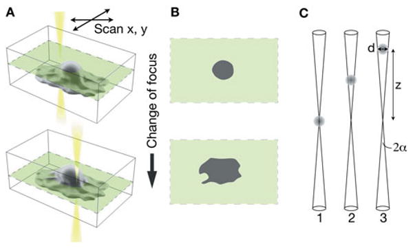
Principle of operation of 3D STEM. A: An image is obtained by scanning the electron beam in the x-y plane at a certain focus position. The focus position is successively changed, and a new image is recorded each time. B: Each two-dimensional image represents a slice of the 3D dataset. C: Schematic representation of the imaging of a particle with diameter d by an electron beam with semiangle α at various positions z with respect to the focal plane.
The optimal spatial resolution of a conventional STEM is determined by the balance between diffraction and spherical aberration of the objective lens. Diffraction leads to a blurring of the spot size inversely proportional to the opening semiangle α. Spherical aberration causes electrons traveling at higher angles to the optical axis to be focused too strongly and increases the spot size proportional to α3. Spherical aberration correction in STEM allows larger opening angles to be used, thereby decreasing the blurring effect of diffraction until a balance is reached with the next limiting aberration. The three major benefits of spherical aberration correction are (1) a decrease of the size of the electron probe at the focal point, resulting in a lateral resolution of 0.1 nm or better (Nellist et al., 2004), (2) a better signal-to-noise ratio for the same electron probe current, and (3) a decrease in the depth of field, which is the key effect used in 3D STEM. The diffraction-limited axial resolution is given by (Borisevich et al., 2006):
| (1) |
which approximately equals the full-width at half-maximum (FWHM) of the STEM probe intensity along the optical axis, similar as in light optics. Typical numbers for a conventional STEM are α = 9 mrad and δz = 62 nm at a beam energy U = 200 kV, while state-of-the art aberration-corrected STEM gives α = 45 mrad and δz = 2.5 nm. This definition of the axial resolution assumes that the width of the PSF is approximately equal to, or larger than, the object size. For the imaging of biological specimens such high axial resolution might not always be achievable. The high intensity of the electron beam at the focus prevents the use of cryo-sections and the samples have to be metal-stained. The diameter of the individual grains of the stain is typically in the range of 1–3 nm, which is much larger than the PSF of the aberration-corrected STEM. Figure 1C is a schematic representation of the imaging of a spherical particle imaged with a focused beam of a much smaller size. For a range of focus values, the obtained images will look similar. Based on the argument of shadowing by the metallic grains of the stain, the axial resolution becomes
| (2) |
with d the diameter of a spherical grain. For grains of sizes of 1–3 nm, the axial resolution is thus expected to be in the range of δz = 22–67 nm for α = 45 mrad, provided flat phase conditions are achieved across the whole aperture. Equation (2) is consistent with calculations of the contrast transfer function in the presence of objects larger than the PSF and with measurements on 4, 6, and 8 nm diameter nanoparticles (Behan et al., 2009; Xin & Muller, 2009). Furthermore, the highest axial resolution as predicted by equation (1) can only be achieved when the pixel size is smaller than the PSF. For the typical microscope settings used to image biological specimen, this is not the case and under-sampling occurs (Pawley, 1995). In cases where the grain size is smaller than the pixel size, equation (2) predicts the axial resolution when d is replaced by the pixel size. Other effects, such as radiation damage, limiting the available electron dose, also influence the obtainable resolution. For biological specimens it is important to realize that the obtainable axial resolution is sample related.
Materials and Methods
Sample Preparation
The cytoskeleton samples were prepared with a platinum rotary shadowing method (Svitkina et al., 1995), resulting in metallic replicas of the biological structure with a high stability under electron beam irradiation. The Madin-Darby canine kidney (MDCK) cells were extracted with 1% Triton X-100 in cytoskeleton stabilization buffer. Cells were washed with wash buffer and then fixed with 2% glutaraldehyde in water for 40 min, followed by 2% tannic acid and 0.1% uranyl acetate for 20 min each. Samples were dehydrated in increasing concentrations of ethanol and critical point dried. Platinum rotary shadowing was followed by carbon shadowing. Replicas were floated and mounted on carbon copper grids, and 15 nm gold particles were adsorbed onto the replica. Prior to STEM imaging the sample was plasma cleaned.
The 3T3 cells were fixed with glutaraldehyde, stained with reduced osmium, embedded in epoxy resin, and contrasted with lead (Glauert & Lewis, 1998). Thin sections (0.15 μm) were cut using an ultramicrotome. Gold nanoparticles were put on both sides of the section. The sections were covered with a thin film of amorphous carbon (10 nm thickness) on both sides, to reduce the possible damaging effects of electrical charging. The sample was placed in high vacuum for several days to reduce the effect of contamination during imaging.
Electron Microscopy
MDCK cells were imaged at 200 kV with an aberration-corrected STEM/TEM (JEOL 2200FS) using the annular dark field detector. The corrector was aligned on the same day as the measurements for a semiangle of 41 mrad of the electron beam. A total of 220 images of 512 × 512 pixels were recorded in a focal-series with a pixel size of 0.55 nm and each image differing 1 nm in focus. A pixel dwell time of 5 μs and a probe current of 30 pA were used. The total imaging time was 5 min. The lateral drift was less than 5 nm over the entire dataset. The drift in focus position of the microscope was measured on a different sample and found to be less than 1 nm/min, which can be neglected.
The 3D dataset recorded at a semiangle of 26.5 mrad had 1,024 × 1,024 pixels, a pixel size of 0.28 nm, a focus step of 5 nm, and a pixel dwell time of 10 μs. The 3D dataset recorded at a semiangle of 17.7 mrad had 512 × 512 pixels, a pixel size of 0.55 nm, a focus step of 5 nm, and a pixel dwell time of 32 μs.
The 3D STEM dataset of the 3T3 cell was recorded at the position of a Golgi ribbon with a semiangle of 41 mrad and a 200 kV electron beam. A total of 150 images of 512 × 512 pixels were recorded in a focal-series with a pixel size of 0.55 nm and each image differing 2 nm in focus position. A pixel dwell time of 10 μs and a probe current of 30 pA were used.
Tilt series were recorded with a 200 kV TEM (FEI company Tecnai 20) with 87 different tilt angles following the Saxton scheme, a total tilt range of ± 65°, and a recording time of 1 h. The defocus was − 1 μm.
Data Processing
The following four steps were applied to align the 3D dataset of the MDCK cells. First, the noise in each image was reduced using a convolution filter (kernel: 1,1,1; 1,5,1; 1,1,1) using Digital Micrograph software (Gatan). The dataset was then compensated for changes of the average detector signal per image with the optical density correction procedure in Autoquant software (Media Cybernetics Inc.). Finally, the 3D dataset was automatically aligned slice-by-slice including a compensation for small image deformation (Autoquant settings: normal warp severity and alignment compare to neighbor), and cropped to 490 × 490 pixels. The contrast and brightness were adjusted for maximal visibility.
The 3D STEM dataset of the 3T3 cells was processed as follows. The noise in each image was reduced using a convolution filter (kernel: 1,1,1; 1,5,1; 1,1,1) using Digital Micrograph software (Gatan). The 3D dataset was aligned in two steps. The first step was alignment of the lateral drift of the specimen (without compensating for sample deformation). The dataset was then cropped to remove the first 30 last 20 images (sample shrinkage was observed for the first 30 images). The second alignment step included compensation for sample deformation and STEM scanning distortion (Autoquant settings: tiny warp and align compare to neighbor).
The tomogram was reconstructed using the weighted back projection algorithm implemented in IMOD (Kremer et al., 1996).
Results
The 3D STEM datasets of the cytoskeleton of MDCK cells were recorded at 200 kV with an aberration-corrected STEM. This type of sample can be used to study the cytoskeleton (Burnette et al., 2007). The 3D dataset was processed in an automated procedure to correct for lateral drift and changes occurring from frame to frame such as scan distortion and sample deformation. The lateral drift was maximal 5 nm. Figure 2 shows two horizontal slices of the aligned 3D dataset containing a clathrin-coated pit formed by endocytosis at the cell surface and parts of the cytoskeleton. The two slices differ 67 nm in focus (vertical) position. The top surface of the clathrin-coated pit is visible in-focus in Figure 2A, while the cytoskeleton is visible in-focus in Figure 2B. These images demonstrate that 3D sensitivity was obtained and that the individual grains of the platinum stain were resolved in the lateral plane. The original 3D dataset is shown in Supplementary Movie 1.
Figure 2.
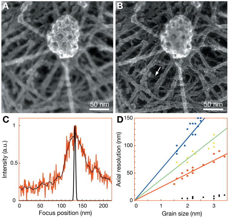
3D STEM images of a clathrin-coated pit and parts of the cytoskeleton of MDCK cells. Panels A and B are at the same lateral (horizontal) position, but differ by 67 nm in focus (vertical position). The 3D dataset was aligned in the horizontal plane. The beam semiangle was 41 mrad. C: Line scan in the vertical direction over the grain indicated by the arrow in panel B (red). The noise of the line scan was reduced by averaging adjacent pixels (4 above and 4 below) (thin black line). The line scan at the same position in the deconvolved 3D dataset is also shown (thick black line). D: The axial resolution was determined as a function of grain size for several particles and for three different beam semiangles, 41 mrad (red), 26.5 mrad (green), and 17.7 mrad (blue). The theoretical prediction is shown as lines of the corresponding colors. The full-width at half-maximum measured on the same grains but after deconvolution is shown as black squares.
A total of 17 staining grains were analyzed to determine the resolution achieved. Figure 2C shows a vertical line scan (intensity versus axial position) obtained at the grain indicated by the arrow in Figure 2B. A significant degree of noise is visible, and the background signal does not evolve to zero at higher or lower a. Averaging adjacent data points reduced the noise, and the FWHM of the peak above the background level was determined to 55 nm. We take the FWHM of the vertical line scan as a measure of the axial resolution δz obtained on this particular grain. The FWHM in the lateral plane of this grain was 2.2 nm (data not shown), which measures the size of the grain. The 3D dataset was recorded with a pixel size (0.55 nm) larger than the electron probe size leading to undersampling. Following the Nyquist criterion (Pawley, 1995), the lateral (horizontal) resolution thus amounted to 2 × 0.55 nm = 1.1 nm. The axial resolution follows a linear curve with grain size as expected on the basis of equation (2). Additional 3D data-sets were recorded at two different beam semiangles, 17.7 and 26.5 mrad. Totals of 15 and 10 grains, respectively, were analyzed (see Fig. 2D). Also for these angles the axial resolution is in accordance with the expected values based on equation (2).
The images from a 3D focal-series contain both the in-focus information from the focal plane as well as out-of-focus contributions from objects above and below the focal plane. Crucial for 3D wide field microscopy is deconvolution (Pawley, 1995). In the case of incoherent imaging, the image I is a convolution of the object O with the PSF (Puetter et al., 2005):
| (3) |
In this equation, x and y are three-dimensional vectors. The imaging process also adds noise N (x). When imaging a thin object, the PSF becomes approximately invariant of the position and can be written as a 3D matrix of the displacement PSF (x-y). Deconvolution is the reverse process used to obtain a model of the original shape by calculation. Without noise, deconvolution of the image can lead to ultrahigh so-called superresolution (Carrington et al., 1995). But often, noise is limiting the resolution, and the present deconvolution algorithms therefore include estimates of the noise statistics. Here, an iterative blind deconvolution using a maximum-likelihood approach was adapted for 3D STEM to resolve the vertical information. 3D STEM deconvolution was implemented in Autoquant software (Media Cybernetics Inc.). The deconvolution procedure consisted of four steps: (1) both the object and the PSF were estimated in 50 iterations of adaptive deconvolution, (2) the object estimate was refined by 50 iterations of deconvolution with a fixed PSF, (3) 50 iterations of adaptive axial deconvolution were applied, and (4) 25 iterations with a fixed PSF completed the deconvolution.
Figure 3A–C show three horizontal slices of the deconvolved 3D dataset of Figure 2, each differing 20 nm in focus (vertical) position. The top surface of the clathrin-coated pit can be seen in Figure 3A, the sidewall of the pit in Figure 3A, and the supporting cytoskeleton in Figure 3C. The entire deconvolved 3D dataset is shown in Supplementary Movie 2.
Figure 3.
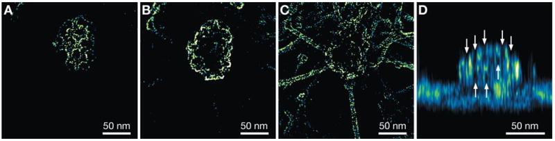
3D reconstruction of a clathrin-coated pit and parts of the cytoskeleton of MDCK cells obtained via deconvolution. The signal level is color-coded. A–C: Horizontal slices of the 3D dataset differing by 20 nm in vertical position. The gamma value of the images was adjusted to 0.5 to improve the visibility of the surface. D: Side view projection of the xz plane consisting of the average signal of all slices along the y direction. The arrows point to openings in the honeycomb mesh of the pit.
The lateral resolution is sufficient to resolve the individual grains of the platinum stain. Figure 3D is a side view through the entire dataset demonstrating that the FWHM of the nanoparticles has been greatly reduced in the axial direction as well. The spatial arrangement of the clathrin molecules leads to the formation of a polyhedral lattice appearing as a hexagonal honeycomb pattern. The openings of this mesh are visible from the top in Figure 3A and from the side in Figure 3D.
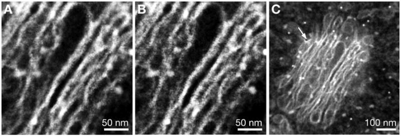
The FWHMs of the vertical line scans were determined over the same grains before and after deconvolution (Fig. 2D). The average value of the FWHM after deconvolution was 6 nm, demonstrating the effectiveness of the deconvolution (one example is shown as the thick line in Fig. 2C). To evaluate the axial resolution of the deconvolved dataset, we searched the 3D dataset for two grains with the same horizontal coordinate, but with different heights. In Figure 4A,B, two images are shown depicting parts of the cytoskeleton below the clathrin coated pit and differing 11 nm in axial position. On the right side, two overlapping filaments are seen. Each filament is coated by Pt grains, whose line-shaped pattern can be followed along the dashed lines. At the position of the arrow, two grains exist with a similar lateral position, i.e., the positions with maximum intensity differing only 1 pixel in the xy plane. Figure 4C, the image in the xz plane at the same y position, shows that the grains are on top of each other. The vertical line scan in Figure 4D exhibits two peaks differing by 11 nm in vertical position and each having a FWHM of 8 nm. Between the two peaks the signal dips by more than 20% and thus the Raleigh criterion for resolution is satisfied. Vertically overlapping grains at several other positions were analyzed, and four further positions were found with a peak-to-peak distance of 10 ± 1 nm, and a signal dip of more than 20%. We thus conclude that the axial resolution after deconvolution was 10 ±1 nm.
Figure 4.
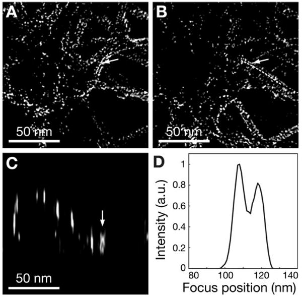
Evaluation of the axial resolution of the deconvolved 3D STEM dataset. Panels A and B are sections of the cytoskeleton just below the clathrin-coated pit differing 11 nm in vertical position. The dashed lines are guides to the eye along sections of two crossing filaments. The arrows point to the same pixel. The gamma value of the images was adjusted to 0.5. C: xz image at the y-coordinate of the arrowed pixel in A and B. Two vertically overlapping grains can be seen at the arrow. D: Vertical line scan at the position of the arrow in C.
The precision of the height location can be determined from the fitting of Gaussians to the two peaks (e.g., in Fig. 4D) and is naturally much higher than the resolution of the original dataset and indeed higher than that of the reconstruction because it uses the entire curve to accurately locate the peak position. The precision for the height of each particle was determined to be ±0.1 nm and ±0.2 nm for the left and the right peak, respectively. The precision was the standard deviation of the results of three fits, where the fit range for the left peak, the intermediate region, and the right peak was each time changed by 1 nm (the standard error of each individual fit was smaller than 0.1 nm).
For comparison we have also recorded tilt-series TEM images of the same sample and generated a 3D tomography reconstruction. The comparison between 3D STEM and tilt-series TEM is depicted in Figure 5. Three different projections (xy, xz, and yz) of the 3D STEM dataset show the side wall and the hollow interior of the clathrin-coated pit (Fig. 5A,C,D). The horizontal slice was located 10 nm in vertical position between the images (Fig. 3B,C). Figure 5E,G,H shows the same projections of a similar clathrin-coated pit imaged on the same sample with tilt-series TEM. Here, the top surface of the clathrin-coated pit is shown, similar to the image in Figure 3A. The resolution of the tomogram was 2 nm in the lateral plane and 3 nm in the axial direction, as determined from the average FWHM of three of the smallest particles. The nanometer scale axial resolution is visible from the side projections. The 3D STEM data contain regions with a higher density of grains leading to a larger scattering of the electron beam visible as bright areas in the image. In those regions the resolution was lower. The tomogram also exhibited regions where the resolution was lower because of local high particle density. For comparison of the images in the horizontal plane, the fast Fourier transformed (FFT) images of Figure 5C,G are shown in Figure 5B,F, respectively. The occurrence of a dark cone in Figure 5F indicates missing information (spatial frequencies) in the FTT of the tomography reconstruction. The missing cone of the STEM reconstruction is not in the lateral plane but in the out of plane information (Behan et al., 2009; Xin & Muller, 2009).
Figure 5.
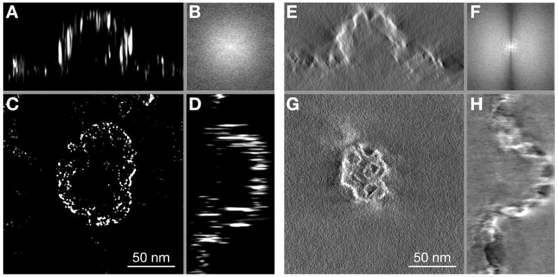
Comparison of 3D STEM and tilt-series TEM using similar clathrin-coated pits imaged on the same sample. Panels A, C, and D are the xz, xy, and yz projections, respectively, of the deconvolved 3D STEM dataset. The xy projection represents one slice positioned 10 nm in focus (vertical) position between the images of Figure 3B,C. The xz and yz projections are the averages of 10 slices in the y and x directions, respectively. The corresponding projections of the tilt-series TEM dataset are shown in E, G, and H. Also here, the xz and yz projections are the averages of 10 slices in y and x direction, respectively. B: FFT of image C. F: FFT of image G.
Three-dimensional STEM images were also recorded of thin sections containing mammalian cells (NIH 3T3, mouse fibroblast cell line) to investigate the obtainable resolution on conventional thin sections that are subject to radiation damage. The 3D dataset was aligned in an automated procedure. The maximal lateral drift was 8 nm, and the maximal sample distortion was 3 nm. The resulting 3D dataset appeared to be free from drift and distortion in the lateral plane. However, vertical distortion cannot be compensated for by this method. Figure 6A,B shows two slices of the 3D dataset differing 60 nm in vertical position. The Golgi apparatus appears as a stack of saccules (i.e., cisternae). Different sections are in focus in each image, thus demonstrating the depth sensitivity of 3D STEM on this specimen. After the recording of the 3D dataset, a single image was recorded at a lower magnification. Figure 6C shows that several beam damage effects occurred. A small hole appeared in the sample at the position of the arrow; presumably the beam was parked at that position between recording the images of the 3D dataset. Note that this type of beam damage can be easily avoided by using beam blanking between the scans (not yet available for our microscope). The area in the middle shows a white square, which is considered to be a layer of deposited amorphous carbon contamination. The overall shape, however, is still mostly intact (apart from a small degree of shrinkage). Thus, it can be concluded that 3D STEM imaging of conventional thin sections is possible.
Figure 6.
3D STEM imaging of a Golgi stack in a conventional thin section containing 3T3 cells. A,B: Two images of the aligned dataset differing 60 nm in vertical position. The curves of the images were adjusted for maximal contrast. C: STEM image recorded after recording the 3D dataset.
The 3D dataset was deconvolved with a procedure consisting of three steps: (1) both the object and the PSF were estimated in 100 iterations of adaptive deconvolution, (2) the object estimate was refined by 500 iterations of deconvolution with a fixed PSF, and (3) 10 iterations of adaptive axial deconvolution were applied. Figure 7A–C shows three slices of the deconvolved 3D dataset each differing 30 nm in vertical position. In each image a different section of the Golgi ribbon is observed. The axial FWHM of the reconstruction was determined from 10 grains and amounted to 11.4 nm, indicating that the axial resolution was comparable to that of the deconvolved 3D dataset of the cytoskeleton (Fig. 3). The lateral resolution was again defined by the pixel size and was 1.1 nm.
Figure 7.
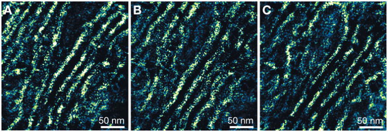
Deconvolved 3D STEM images of the Golgi. A–C: Images of the deconvolved dataset each differing 30 nm in vertical position. The gamma of images was set to 0.5. Panels A and C are at the same vertical position as panels A and B of Figure 6, respectively.
Discussion
The 3D STEM dataset of the cytoskeleton of MDCK cells exhibited a pixel-limited lateral resolution of 1.1 nm and a specimen-limited axial resolution of several tens of nanometers depending on the grain size of the Pt nanoparticles used for staining. After reconstruction, the axial resolution through small grains improved to an average value of 10 nm for the cytoskeleton sample that showed high radiation stability. This is comparable with tilt-series TEM results on the same sample, roughly a factor of 2 better in the lateral plane and a factor of 3 worse in the axial direction.
Before reconstruction two grains of 2 nm diameter lying directly above each other would not be resolvable unless they were vertically spaced by 44 nm (for α = 45 mrad) following equation (2). Figure 4 shows that two grains differing 11 nm in vertical position can be distinguished in vertical direction after deconvolution, according to the Raleigh criterion. This was possible because the center of intensity differed by just 1 pixel in the horizontal direction. The deconvolution locates the vertical position of each grain with a precision of ±0.2 nm for small grains. It is important to realize that because the lateral resolution is good, grains usually are separated sufficiently in the lateral plane that there rarely are multiple grains present in the exact same axial profile. So in most cases grains on, say, a back surface and front surface can be isolated. A dataset with 512 × 512 horizontal coordinates of 0.5 nm and 200 vertical coordinates of 1 nm could resolve approximately 128 × 128 × 20 = 3 × 10⁵ grains of 2 nm diameter. This number should be sufficient to resolve stained 3D objects with nanometer resolution. However, the sample preparation requires optimization toward small and homogeneously distributed grains.
We should also mention that no explicit constraint was used for the deconvolution. The distribution of staining grains was sparse enough that there was almost always lateral separation. The high lateral resolution enabled the deconvolution to separate staining grains in 3D space. The deconvolution could possibly be improved by introducing the minimum structure in the object as constraint, which is frequently used in maximum entropy methods. The deconvolution procedure could detect an axial response that exceeds the PSF and then assign two objects to account for the observed intensity distribution. Mathematically there are an infinite number of object distributions that could account for the observation. Sometimes the less likely solutions, such as the existence of three vertically aligned smaller particles, will be the true situation, but infrequent errors of this nature should not affect the overall reconstructed 3D shape of the object.
The consistency of the data with the theoretically predicted values of the axial resolution of equation (2) supports the idea that subnanometer axial resolution can be achieved by developing samples with smaller grains and by using deconvolution. Optimized 3D STEM on small samples, e.g., negatively stained protein complexes, or viruses, is expected to facilitate single particle tomography (Frank, 2006), for example, by determining the symmetry of a 3D structure, or to identify the existence of subunits of protein complexes. The theoretical maximum axial resolution on objects smaller than the PSF with 41 mrad beam semiangle is 2.5 nm before deconvolution. Optimization of the settings of toward larger opening angles is possible using higher-order aberration correctors (Haider et al., 2000), with values of α = 50 to 70 mrad, leading to δZ approaching 1 nm. Further resolution improvements can be obtained by optimizing the deconvolution software, or by combining 3D STEM datasets obtained at several tilt angles, e.g., + and −20°. A key advantage of the 3D STEM wide field microscopy technique is efficient use of the available electron dose. The deconvolution process applied here uses all information (also the out-of-focus information) for the 3D reconstruction, which essentially leads to a noise reduction (see Fig. 2C).
The imaging of biological specimens is typically limited by radiation damage. For TEM imaging of a specimen of Araldite resin, the total dose can amount up to 4 × 10⁵ e−/nm2 (Luther et al., 1988). In a typical TEM experiment, the sample is preirradiated with a dose of approximately 104 electrons/nm2, leading to a rapid shrinkage of the sample by about 20% of its original thickness and 10% of its lateral dimension, followed by a period with relative stability of the sample (Luther et al., 1988). Due to the staining artifacts and the shrinkage, the images obtained with a conventional thin section do not represent the native state but still allow investigation of the ultrastructure of the sample (Bozzola & Russell, 1992). The total electron dose used in the 150 images of the 3D STEM dataset was 9 × 10⁵ electrons/nm2 (the total number of electrons through the sample divided by the radiated area of the specimen). Sample shrinkage was observed for the first 30 images (1.9 × 10⁵ electrons/nm2), and the remaining 100 images of the cropped 3D dataset occurred while the sample was stable to within 3 nm in the lateral plane. This sample behavior during STEM imaging is consistent with TEM imaging. The obtained lateral resolution on the conventional thin section of 1.1 nm was already more than needed to resolve the grains of the osmium and lead staining. The axial resolution of 3D STEM obtained on the conventional thin section was about a factor of 4 worse than that of tilt-series TEM of the Golgi apparatus (Marsh et al., 2004). Additional deconvolution steps did not yield a better axial resolution and led to the removal of the small-sized grains. A possible explanation for the limited result of the deconvolution on this specimen is the deformation of the specimen during imaging, which also occurs for tilt-series TEM (Luther et al., 1988; Bozzola & Russell, 1992). For tilt-series TEM a high-resolution tomography reconstruction is still possible despite sample shrinkage. For the current deconvolution method to converge to higher resolution, however, it is required that the 3D shape of the specimen remains highly stable during data acquisition. The resolution can possibly be improved by developing 3D alignment algorithms that compensate not only for lateral deformation but also for axial deformation. Second, the deconvolution algorithm tends to remove small-sized grains. Optimization of the deconvolution software could possibly result in a higher axial resolution while maintaining the fine features in the image. Furthermore, the grain size of the conventional thin section could possible be reduced by adapting the sample preparation protocol.
The 3D STEM exhibits several advantages over tilt-series TEM due to the absence of mechanical tilt:
Tilt-series TEM suffers from missing information due to the missing wedge, or cone in the reconstruction, and a range of spatial frequencies is absent in the data, even in horizontal (xy) slices (Bartesaghi et al., 2008). The 3D STEM, on the contrary, contains all the information in horizontal slices (see Fig. 5B). The 3D STEM misses information in the vertical (z) direction due to shadowing and the missing cone is much larger (Behan et al., 2009; Xin & Muller, 2009) than for tomography. Thus, while one wins in the horizontal direction, one looses in the vertical direction. The specimen is not tilted in 3D STEM.
Tilt-series TEM has a limited resolution with thick specimens. The effective thickness of the specimen as “seen by the electron beam” increases as the section is tilted from 0 to 70° (a factor of 3 increase).
The total area that can be imaged with tilt-series TEM is limited (a) by the amount of pixels in the TEM camera (modern charge couple device cameras have up to 8,000 × 8,000 pixels) and (b) by the maximal focus change in one image that can be compensated for, i.e., 3 μm is already required for an image size of 10 × 10 μm at 70° tilt [note that tilt-series STEM is capable of correcting for defocus (Kuebel et al., 2005) and can be used to image specimen of up to a micrometer thickness (Hohmann-Marriott et al., 2009)]. The 3D STEM collects an image pixel-by-pixel (there is no limitation due to the size of the camera) and without the need of tilt. Large images can thus be recorded simply by deflecting the beam and even larger images can be acquired by combining horizontal stage movements with the beam scanning. Therefore, it is possible in principle to record very large datasets containing, for example, several adjacent cells, by a combination of precise stage movement and the scanning of large areas. The size of the area of a 3D STEM image is determined in the end by the amount of data that can be handled by the computer used for deconvolution. Note that the imaging time increases with increasing image size, which can be partly compensated by using a higher probe current and smaller pixel dwell time.
Of importance is also the order of magnitude shorter time required to record the data, making it suitable for high-throughput imaging. The 3D STEM imaging and data processing are already implemented in a fully automated procedure.
Finally, the contrast mechanism of STEM can be used to detect nanometer-sized particles of materials of a high atomic number inside an embedding medium of a low atomic number (Sousa et al., 2008). Different proteins in cells can thus be specifically labeled (Xiao et al., 2003) and detected in 3D. The total level of staining, e.g., with osmium compounds, should be kept small enough, or entirely avoided, for the labels to be visible in the background signal. In the future, sparse or protein-specific labeling could allow 3D STEM to be extended to much thicker specimens, and even to whole cells in liquid (de Jonge et al., 2009).
Conclusions
The 3D STEM already has a resolution comparable with tilt-series TEM on the same sample (a metal replica of the cytoskeleton of MDCK cells), and the resolution can theoretically be increased by optimizing the sample preparation method, optimizing the deconvolution software, and by using larger beam semiangles. A 3D STEM dataset can be recorded with an electron dose comparable to that used for conventional thin sections. The focal-series method has several advantages over tilt-series TEM, such as an order of magnitude faster imaging and the absence of mechanical tilt. The 3D STEM is potentially capable of imaging biological specimens with subnanometer resolution, of imaging very large areas and can be used for the 3D imaging of whole cells.
Supplementary Material
Acknowledgments
We thank L.F. Allard, D. Blom, J.F. Deatherage, A.R. Lupini, and J.R. Price for discussions and help with the experiments, and J. Swan and B. Twomey for help with Figure 1. This work was supported by the Laboratory Directed R&D Program of Oak Ridge National Laboratory (N.J.), by the High Temperature Materials Laboratory, sponsored by the U.S. Department of Energy, Office of Energy Efficiency and Renewable Energy, Vehicle Technologies Program, by Vanderbilt University Medical Center, National Institutes of Health grant R01GM081801 (N.J.), by the Intramural Program of NICHD (R.S.), and by the U.S. Department of Energy Office of Science, Division of Materials Science and Engineering (S.J.P.).
References
- Bartesaghi A, Sprechmann P, Liu J, Randall G, Sapiro G, Subramaniam S. Classification and 3D averaging with missing wedge correction in biological electron tomography. J Struct Biol. 2008;162:436–450. doi: 10.1016/j.jsb.2008.02.008. [DOI] [PMC free article] [PubMed] [Google Scholar]
- Behan G, Cosgriff EC, Kirkland AI, Nellist PD. Electron microscopein the aberration-corrected scanning transmission three-dimensional imaging by optical sectioning. Phil Trans R Soc A. 2009;367:3825–3844. doi: 10.1098/rsta.2009.0074. [DOI] [PubMed] [Google Scholar]
- Borisevich AY, Lupini AR, Pennycook SJ. Depth sectioning with the aberration-corrected scanning transmission electron microscope. Proc Natl Acad Sci. 2006;103(9):3044–3048. doi: 10.1073/pnas.0507105103. [DOI] [PMC free article] [PubMed] [Google Scholar]
- Bozzola JJ, Russell LD. Electron Microscopy. Boston, MA: Jones and Bartlett Publishers; 1992. [Google Scholar]
- Burnette DT, Schaefer AW, Ji L, Danuser G, Forscher P. Filopodial actin bundles are not necessary for microtubule advance into the peripheral domain of Aplysia neuronal growth cones. Nat Cell Biol. 2007;9(12):1360–1369. doi: 10.1038/ncb1655. [DOI] [PubMed] [Google Scholar]
- Carrington WA, Lynch RM, Moore EDW, Isenberg G, Fogarty KE, Fay FS. Superresolution three-dimensional images of fluorescence in cells with minimal light exposure. Science. 1995;268:1483–1487. doi: 10.1126/science.7770772. [DOI] [PubMed] [Google Scholar]
- de Jonge N, Peckys DB, Kremers GJ, Piston DW. Electron microscopy of whole cells in liquid with nanometer resolution. Proc Natl Acad Sci. 2009;106:2159–2164. doi: 10.1073/pnas.0809567106. [DOI] [PMC free article] [PubMed] [Google Scholar]
- de Jonge N, Sougrat R, Peckys DB, Lupini AR, Pennycook SJ. 3-dimensional aberration corrected scanning transmission electron microscopy for biology. In: Vo-Dinh T, editor. Nanotechnology in Biology and Medicine-Methods, Devices and Applications. Boca Raton, FL: CRC Press; 2007. pp. 13.1–13.27. [Google Scholar]
- Frank J. Three-Dimensional Electron Microscopy of Macromolecular Assemblies—Visualization of Biological Molecules in Their Native State. Oxford, UK: Oxford University Press; 2006. [Google Scholar]
- Frigo SP, Levine ZH, Zaluzec NJ. Submicron imaging of buried integrated circuit structures using scanning confocal electron microscopy. Appl Phys Lett. 2002;81:2112–2114. [Google Scholar]
- Glauert AM, Lewis PR. Biological Specimen Preparation for Transmission Electron Microscopy. London: Portland Press; 1998. [Google Scholar]
- Haider M, Uhlemann S, Zach J. Upper limits for the residual aberrations of a high-resolution aberration-corrected STEM. Ultramicroscopy. 2000;81:163–175. doi: 10.1016/s0304-3991(99)00194-1. [DOI] [PubMed] [Google Scholar]
- Hell SW. Far-field optical nanoscopy. Science. 2007;316:1153–1158. doi: 10.1126/science.1137395. [DOI] [PubMed] [Google Scholar]
- Hohmann-Marriott MF, Sousa AA, Azari AA, Glushakova S, Zhang G, Zimmerberg J, Leapman RD. Nanoscale 3D cellular imaging by axial scanning transmission electron tomography. Nat Methods. 2009;6(10):729–731. doi: 10.1038/nmeth.1367. [DOI] [PMC free article] [PubMed] [Google Scholar]
- Kremer JR, Mastronarde DN, McIntosch JR. Computer visualization of three-dimensional image data using IMOD. J Struct Biol. 1996;116:71–76. doi: 10.1006/jsbi.1996.0013. [DOI] [PubMed] [Google Scholar]
- Kuebel C, Voigt A, Schoenmakers R, Otten M, Su D, Lee TC, Carlsson A, Bradley J. Recent advances in electron tomography: TEM and HAADF-STEM tomography for materials science and semiconductor applications. Microsc Microanal. 2005;11:378–400. doi: 10.1017/S1431927605050361. [DOI] [PubMed] [Google Scholar]
- Lucic V, Foerster F, Baumeister W. Structural studies by electron tomography: From cells to molecules. Annu Rev Biochem. 2005;74:833–865. doi: 10.1146/annurev.biochem.73.011303.074112. [DOI] [PubMed] [Google Scholar]
- Luther PK, Lawrence MC, Crowther RA. A method for monitoring the collapse of plastic sections as a function of electron dose. Ultramicroscopy. 1988;24:7–18. doi: 10.1016/0304-3991(88)90322-1. [DOI] [PubMed] [Google Scholar]
- Marsh BJ, Volkmann N, McIntosh JR, Howell KE. Direct continuities between cisternae at different levels of the Golgi complex in glucose-stimulated mouse islet beta cells. Proc Natl Acad Sci USA. 2004;101(15):5565–5570. doi: 10.1073/pnas.0401242101. [DOI] [PMC free article] [PubMed] [Google Scholar]
- Meyer-Ilse W, Hamamoto D, Nair A, Lelievre SA, Denbeaux G, Johnson L, Pearson AL, Yager D, Legros MA, Larabell CA. High resolution protein localization using soft X-ray microscopy. J Micros. 2001;201(3):395–403. doi: 10.1046/j.1365-2818.2001.00845.x. [DOI] [PubMed] [Google Scholar]
- Nellist PD, Behan G, Kirkland AI, Hetherington CJD. Confocal operation of a transmission electron microscope with two aberration correctors. Appl Phys Lett. 2006;89:124105-1–124105-3. [Google Scholar]
- Nellist PD, Chisholm MF, Dellby N, Krivanek OL, Murfitt MF, Szilagyi ZS, Lupini AR, Borisevich A, Sides WH, Pennycook SJ. Direct sub-angstrom imaging of a crystal lattice. Science. 2004;305:1741. doi: 10.1126/science.1100965. [DOI] [PubMed] [Google Scholar]
- Pawley JB. Handbook of Biological Confocal Microscopy. New York: Springer; 1995. [Google Scholar]
- Puetter RC, Gosnell TR, Yahil A. Digital image reconstruction: Deblurring and denoising. Annu Rev Astron Astrophys. 2005;43:139–194. [Google Scholar]
- Sousa AA, Hohmann-Marriott M, Aronova MA, Zhang G, Leapman RD. Determination of quantitative distributions of heavy-metal stain in biological specimens by annular dark-field STEM. J Struct Biol. 2008;162:14–28. doi: 10.1016/j.jsb.2008.01.007. [DOI] [PMC free article] [PubMed] [Google Scholar]
- Stahlberg H, Walz T. Molecular electron microscopy: State of the art and current challenges. ACS Chem Biol. 2008;3:268–281. doi: 10.1021/cb800037d. [DOI] [PMC free article] [PubMed] [Google Scholar]
- Svitkina TM, Verkhovsky AB, Borisy GG. Improved procedures for electron microscopic visualization of the cytoskeleton of cultured cells. J Struct Biol. 1995;115:290–303. doi: 10.1006/jsbi.1995.1054. [DOI] [PubMed] [Google Scholar]
- Takeguchi M, Hashimoto A, Shimojo M, Mitsuishi K, Furuya K. Development of a stage-scanning system for high-resolution confocal STEM. J Electron Microsc (Tokyo) 2008;57(4):123–127. doi: 10.1093/jmicro/dfn010. [DOI] [PubMed] [Google Scholar]
- Van Benthem K, Lupini AR, Kim M, Baik HS, Doh SJ, Lee JH, Oxley MP, Findlay SD, Allen LJ, Pennycook SJ. Three-dimensional imaging of individual hafnium atoms inside a semiconductor device. Appl Phys Lett. 2005;87:034104-1–034104-3. [Google Scholar]
- Xiao Y, Patolsky F, Katz E, Hainfeld JF, Willner I. “Plugging into enzymes”: Nanowiring of redox enzymes by a gold nanoparticle. Science. 2003;299:1877–1881. doi: 10.1126/science.1080664. [DOI] [PubMed] [Google Scholar]
- Xin HL, Muller DA. Aberration-corrected ADF-STEM depth sectioning and prospects for reliable 3D imaging in S/TEM. J Electron Microsc. 2009;58:157–165. doi: 10.1093/jmicro/dfn029. [DOI] [PubMed] [Google Scholar]
Associated Data
This section collects any data citations, data availability statements, or supplementary materials included in this article.