Boolean Modeling of Neural Systems with Point-Process Inputs and Outputs. Part II: Application to the Rat Hippocampus

Abstract

This paper presents a pilot application of the Boolean–Volterra modeling methodology presented in the companion paper (Part I) that is suitable for the analysis of systems with point-process inputs and outputs (e.g., recordings of the activity of neuronal ensembles). This application seeks to discover the causal links between two neuronal ensembles in the hippocampus of a behaving rat. The experimental data come from multi-unit recordings in the CA3 and CA1 regions of the hippocampus in the form of sequences of action potentials—treated mathematically as point-processes and computationally as spike-trains—that are collected in vivo during two behavioral tasks. The modeling objective is to identify and quantify the causal links among the neurons generating the recorded activity, using Boolean–Volterra models estimated directly from the data according to the methodological framework presented in the companion paper. The obtained models demonstrate the feasibility of the proposed approach using short data-records and provide some insights into the functional properties of the system (e.g., regarding the presence of rhythmic characteristics in the neuronal dynamics of these ensembles), making the proposed methodology an attractive tool for the analysis and modeling of multi-unit recordings from neuronal systems in a practical context.

INTRODUCTION

The quantitative understanding of the manner in which information is processed by neuronal ensembles in the form of sequences of action potentials (spike-trains or point-processes) remains a great challenge, especially in the case of multi-unit recordings from highly interconnected neuronal systems. The intrinsic complexity of this problem is compounded by the binary nature of the neuronal signals (spike trains viewed as point-processes) which require specialized mathematical methods of analysis and modeling that are distinct from the methods developed for discretized continuous data. Although considerable progress has been made over the last 40 years in developing modeling methods appropriate for point-process inputs and outputs that employ trigger-threshold operators, the efficacy of these methods remains limited either because they fail to capture the full complexity of the problem (e.g., the conventional “integrate-and-fire” model) or because their application becomes impractical as the number of neuronal units increases due to their inherent complexity (e.g., Hudgkin–Huxley type of models).

The hippocampus is a brain site directly involved in learning and memory. It plays an important role in the encoding and retrieval of information used to perform various behavioral tasks. It is also believed to encode spatial information used for navigation.²² The characteristic anatomy and intrinsic organization of the hippocampus (especially in the areas of the dentate gyrus, CA3 and CA1) facilitate its study as a complex neuronal system from the standpoint of information processing. Its importance for memory function has motivated its study for treating damaged cognitive function in that area.¹ The dense collaterals between pyramidal cells in the dorsal hippocampus (and especially the CA3-to-CA1 projections) have prompted investigators to associate this area to auto-associative memory²³ as the route followed by cortically processed information to form long-term memory¹² and to encode spatial information related to specific behavioral tasks.¹³ Parametric modeling methods (based on differential equations) have been used to describe the hippocampal neural dynamics^15,18,20 but lead to complex representations that are not fully evaluated in terms of their predictive capability.

The use of Volterra-type nonparametric models with predictive capability allows reliable quantification of the underlying dynamics of various hippocampal subsystems. To achieve this goal, we describe the possible causal relationships between the putative input and output point-processes with a mathematical model that is nonlinear (because neuronal systems do not satisfy the principle of linear superposition) and dynamic (in the sense that the effects of the present input spread into the future). These models constitute a key step toward the development of neuroprosthetic platforms that may eventually enable the restoration of lost functionality in damaged hippocampal areas.^1,2,4 Using the Volterra modeling approach, predictive models of the dorsal hippocampus have been obtained by our research group in the context of single-input input and two-input systems^3,6,8–11 Notable is the recent application of Volterra-type multi-input/multioutput modeling methods based on the general methodological framework presented in Marmarelis¹⁶ to multi-unit recordings from the hippocampal CA3 and CA1 regions.^21,25,26 However, the complexity of this latter approach remains considerable and the motivation remains strong for the development of more efficient modeling methods in the context of multi-unit recordings.

This paper presents the results of a pilot application of a new method of modeling neural systems with point-process inputs and outputs that utilizes Boolean operations (logical AND and OR operations). The companion paper (Part I) presents the methodological framework and illustrative results from simulations, and this paper (Part II) presents the corroborating results of an initial application to point-process data recorded from multiple units of the CA3-to-CA1 causal pathway in the rat hippocampus during various behavioral tasks and seeks to examine some key functional characteristics of the causal links between neuronal units in the two regions.

METHODS

This application is motivated by the desire to quantify the multi-unit transformations of neuronal activity between different regions of the hippocampus. To this purpose, multi-unit point-process data from behaving rats are recorded contemporaneously from several spatially-distinct sites at the CA3 and CA1 hippocampal regions, while the rats are performing two distinct behavioral tasks involving memory (see below). The recorded multi-unit data are used to model the nonlinear functional relationship between neuronal ensembles in the CA3 region (input) and the CA1 region (output) during these behavioral tasks, following the novel methodology of Boolean–Volterra modeling presented in the companion paper (Part I).

Experimental Data

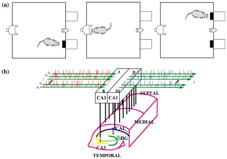
Male Long–Evans rats (n = 5, 3–11 months of age) were trained on a two-lever spatial delayed-nonmatchto-sample (DNMS) task with randomly occurring variable delay intervals of 1–40 s (see Fig. 1a). The animal performs the task by pressing the lever presented in the sample phase (left or right), as indicated in Fig. 1a(I). This constitutes the sample/position information on the trial. The lever is then retracted, and the delay phase initiated, during which the animal must poke its nose into a lighted device on the opposite wall for the duration of the delay, as shown in Fig. 1a(II). After the delay, both levers are extended and the animal must press the lever opposite to the sample/position information (nonmatch response), as indicated in Fig. 1a(III). The longer the delay between trials, the less likely it is that the animal will have the correct response on that trial. Correct responses are rewarded with a drop of water delivered to the trough between both levers during a 10 s inter-trial interval (ITI). Incorrect responses produce a darkened chamber for 5 s without reward, followed by a 5 s ITI. The next trial is initiated after at least 5 s ITI. Only data from correct-response trials were utilized in this study.

FIGURE 1.

(a) Illustration of the behavioral tasks performed by the live rat in each trial of the experiment. (I) right sample, (II) delay phase, (III) left nonmatch; (b) schematic representation of the multi-electrode array recording from the CA3 and CA1 hippocampal regions of the behaving rat.

The datasets used in the cases shown in this paper were chosen from a large database of experimental data acquired by the research group of Prof. Dead-wyler in Wake-Forest University in the context of an effort to develop a cognitive neuroprosthesis testbed. In that study, arrays of 16 microwires (40 μm) were surgically implanted using both stereotaxic coordinates and spontaneous cell firing activity to position the electrode tips in both the CA3 and CA1 cell layers (see Fig. 1b). The arrays were supplied by the NB Labs (Denison, TX, USA) and had the fixed geometry of an orthogonal grid with 200 μm between pairs along the septo-temporal axis and 800 μm between pairs along the medio-lateral axis. The length of the electrode tip was precisely trimmed to follow the longitudinal curvature of the hippocampus.

Data were collected from 11 animals and a total of 198 pyramidal cells (an average of 16–20 simultaneously recorded cells per animal) over at least seven DNMS sessions with stable extracellular action potential waveforms and consistent event-specific firing patterns. Neurons that exhibited low firing rate (<0.2 spikes/s) were excluded as unresponsive. The selection of the specific datasets for the present study was based on the selection algorithm described in Zanos et al.²⁵ A bin-width of 10 ms was used in this study and was selected to be just shorter than the minimum inter-spike interval in these particular sets of experimental data, so that the risk of merging two or more spikes is avoided while computational efficiency is achieved.

Modeling Methodology

The multi-unit point-process data recorded during each of the behavioral tasks (sample and nonmatch) were analyzed with the Boolean–Volterra (B–V) modeling methodology presented in the companion paper (Part I). The first order (excitatory and inhibitory) and the second order B–V kernels were estimated following the “ranking method” that was shown to be reliable in the previously presented study using simulated data (Part I). The predictive performance of the obtained models was evaluated by the figure-of-merit Q that is computed on the basis of the resulting numbers of true-positive and false-positive predictions of output spikes. The parameter value r was computed as the ratio of the input mean firing rate to the output mean firing rate and was used for the evaluation of Q. In the case of multiple inputs, r was computed as the sum of all input mean firing rates over the output firing rate. By computing the r value based on the mean firing rates of the input and output in each case, we allow the ranking algorithm to select the active lags that account for this relation between the input and output mean firing rates.

This study was limited to second-order models (although higher order B–V kernels may exist and should be explored in the future), because its purpose as a pilot application is to demonstrate the efficacy of the proposed B–V modeling approach. The first order B–V kernels describe how input spikes generate output activity (excitatory or inhibitory) and with what latencies. The second order B–V kernels describe the interactions of pairs of input spikes on the output activity in the sense of facilitatory conditioning. In the two-input case, the effect of cross-interactions between the two inputs on the output activity is quantified (modeled) by means of the estimated second order B–V cross-kernel.

The predictive capability of the obtained models is measured through the two performance metrics of True Positives Fraction (TPF) and False Positives Fraction (FPF) which are defined by the following relations:

$$\begin{array}{l}\text{TPF}=\frac{(\text{number}\text{of}\text{TP})}{(\text{number}\text{of}\text{actual}\text{output}\text{spikes})}\\ \text{FPF}=\frac{(\text{number}\text{of}\text{FP})}{(\text{number}\text{of}\text{nonspike}\text{events})}\end{array}$$ (1)

RESULTS

Seventeen cases from eight different experimental preparations (involving three different animals and two distinct behavioral tasks) were considered in our analysis: 13 one-input/one-output cases and four two-input/one output cases (six sample and six nonmatch one-input/one-output cases and two sample and two nonmatch two-input/one-output cases). For each case, the Coincidence Counts (CIs) of the respective first order (excitatory and inhibitory) and second order B–V kernels were computed from the input–output data and the proposed “ranking” method (see Part I) was used to select the “active lags” of the estimated B–V kernels. In evaluating the model predictive performance with the figure-of-merit Q (based on the truepositive and false-positive model predictions), one sample (10 ms) was allowed on either side of the reference sample to account for the effects of possible “jitter” in the location of each predicted spike relative to the respective actual output spike. Possible consecutive predicted spikes, surrounding a true-positive prediction, were counted as false-positive predictions. In each case, the value of parameter r was defined as the ratio of the input mean firing rate (or the sum of these rates in the two-input case) to the output mean firing rate.

One-Input/One-Output Case

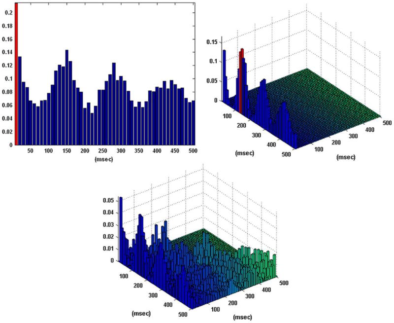
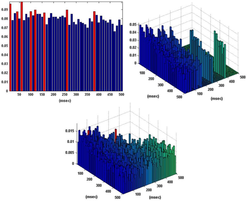
Figure 2 shows the obtained B–V kernels in the one-input/one-output case of a “sample” behavioral task. Note that the computed CIs depict the presence of the “theta rhythm” (a frequency of 7–8 Hz) frequently observed in hippocampal activity. This rhythmic pattern of activity is present in the input data and it is not reflected in the input–output dynamics captured by the obtained kernels. Specifically, only the first lag is selected as an active lag in the first order excitatory B–V kernel (i.e., a simple “relay” characteristic where each input spike generates an output spike with a latency of 10 ms) and the two selected active lags in the first order inhibitory B–V kernel are the 12th and 13th (i.e., an inhibitory latency roughly equal to the period of the theta rhythm). There are no second order interactions in this case, since no active lags were identified in the second order B–V kernel. These results indicate that an output spike is generated by this neuron only when there is an input spike on the first lag without being followed by an input spike on the 12th or 13th lags. This functional characteristic amounts to “filtering” by this neuron of the theta rhythm present in its input. This important point is further discussed in the following section.

FIGURE 2.

The coincidence indices (CIs) for the first order excitatory (left), inhibitory (center), and second order (right) Boolean–Volterra (B–V) kernels of the single-input/single-output case #1 corresponding to a “sample” behavioral task. The computed CIs exhibit a pattern consistent with the “theta rhythm” (7–8 Hz) which is present in the input data. The selected active lags in the first order excitatory and inhibitory B–V kernels are marked with red. No active lags are selected in the second order kernel.

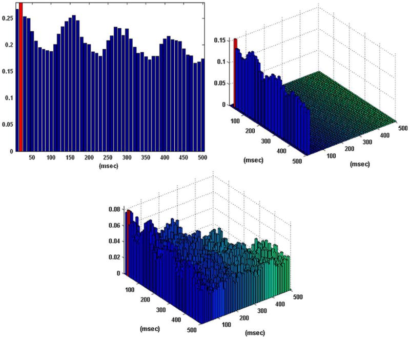
Figure 3 shows the obtained B–V kernels in another case of a “sample” behavioral task, where the computed CIs depict again the presence of the theta rhythm which is present in the input data but it is not reflected in the input–output dynamics, since only the second lag is selected as an active lag in the first order excitatory B–V kernel (i.e., each input spike generates an output spike with a latency of 20 ms) and the only active lag in the first order inhibitory B–V kernel (on the third lag) simply suggests a refractory characteristic. A single active lag is identified in the second order B–V kernel in this case. Its location shows that an output spike is generated when there is a pair of input spikes at lags 1 and 3. These results indicate that an output spike is generated by this neuron in the following two cases: (a) when there is an input spike on the second lag without being followed by an input spike on the third lag (akin to a refractory characteristic); and (b) when there is a pair of input spikes on the first and third lags (akin to facilitatory conditioning). These important points are further discussed in the following section.

FIGURE 3.

The coincidence indices (CIs) for the first order excitatory (left), inhibitory (center), and second order (right) Boolean–Volterra (B–V) kernels of the single-input/single-output case #2 corresponding to a “sample” behavioral task. The CIs of all kernels exhibit the “theta rhythm” (7–8 Hz) which is present in the input data, as in the previous case. The selected active lags in the B–V kernels are marked with red. One active lag is selected in the second order B–V kernel.

Figure 4 shows the obtained B–V kernels for a one-input/one-output case of the other behavioral task (“nonmatch”), where the computed CIs do not depict the presence of the theta rhythm. Note that the complex pattern of the selected active lags in the first order B–V kernel of this “nonmatch” behavioral task may provide indications of the presence of rhythms in the input–output dynamics. For instance, a distance of 20–30 ms between selected active lags (2–3 lags) may reflect the presence of the “gamma rhythm” (30–50 Hz) in the system dynamics, or a distance of 80–120 ms between selected active lags (8–12 lags) may reflect the presence of the “alpha rhythm” (~8–12 Hz). Such inter-lag distances are actually seen in the multiple active lags of the first order B–V kernel for this “nonmatch” behavioral task.

FIGURE 4.

The coincidence indices (CIs) for the first order excitatory (left), inhibitory (right), and second order (center) Boolean– Volterra (B–V) kernels of the single-input/single-output case #5 corresponding to a “nonmatch” behavioral task, along with the selected active lags in the B–V kernels (marked with red). Note that, unlike the previous cases of the “sample” task, the CIs in this case do not exhibit a pattern indicative of the “theta rhythm.” However, the complex pattern of active lags in the first order excitatory B–V kernel may reflect the presence of other rhythms (alpha or gamma) in the system dynamics (see text). No inhibitory lags were selected in this case of a “nonmatch” task. The three active lags selected in the second order B–V kernel cannot be interpreted at this time, although they may generally “detect” the presence and/or interactions between two different rhythms in the input.

Unlike the two cases of the “sample” task shown in Figs. 2 and 3, no active lags are selected in the first order inhibitory B–V kernel of the “nonmatch” behavioral task. Three active lags are selected in the second order B–V kernel of this “nonmatch” task with locations that may generally allow “detection” of the presence and/or interactions between different rhythms in the input. Nonetheless, the potential functional utility of the second order B–V kernel is worth noting and it is further discussed in the following section.

Figure 5 shows the obtained B–V kernels for a one-input/one-output case of the other behavioral task (“nonmatch”). Again, the CIs do not exhibit a clear theta rhythm pattern and the first order B–V kernel contains multiple active lags. Although the precise pattern of active lags in this kernel is different from its counterpart in Fig. 4, the inter-lag distances of these active lags are again suggestive of the presence of possible alpha and gamma rhythms in the system dynamics, for example the distances of 2–4 lags for the gamma rhythm and 8–12 lags for the alpha rhythm.

FIGURE 5.

Another case (#11) of the one-input/one-output “nonmatch” behavioral task, yielding coincidence indices (CIs) and active lags for the first order excitatory (left), inhibitory (right), and second order (center) Boolean–Volterra (B–V) kernels similar to the previous case of Fig. 4. Again, the CIs do not exhibit a clear pattern indicative of the theta rhythm and the first order excitatory B–V kernel has multiple active lags. Although the precise pattern of active lags in this kernel is different from its counterpart in Fig. 4, the inter-lag distances of these active lags are again suggestive of the presence of possible alpha and gamma rhythms in the system dynamics (i.e., distances of 2–4 lags for the gamma rhythm and 8–12 lags for the alpha rhythm). No inhibitory lags and two active lags in the second order B–V kernel were selected in this case. The latter may “detect” the presence and/or interactions between two different rhythms in the input. An initial interpretation of these results is presented in the “Discussion” section.

Two-Inputs/One-Output Case

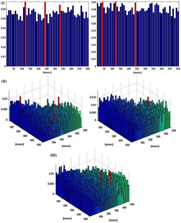
The modeling results for a two-input/one-output case of the “sample” behavioral task are shown in Fig. 6. The two-input model includes two first order B–V kernels (one for each input), their associated inhibitory B–V kernels and three second order B–V kernels of which two are self-kernels (one for each input) and one is the cross-kernel (representing the interactions between the two inputs). The computed CIs do not exhibit any pattern indicative of the theta rhythm in the input, but they may contain hints of higher frequency patterns of input activity.

FIGURE 6.

The computed CIs of the first order kernels (I), the second order B–V self-kernels (II), and the second order B–V cross-kernel (III) for the two-input/one-output case corresponding to a “nonmatch” behavioral task, along with the active lags of the B–V kernels selected by the proposed ranking method (marked with red). No inhibitory active lags were selected in this case and the inhibitory CIs are not shown in the interest of space. The active lags of the first order B–V kernels exhibit a regular pattern consistent with the alpha rhythm (i.e., inter-lag distances of 80–120 ms, corresponding to frequencies of 8–12 Hz). There is no clear pattern in the sparse active lags selected in the second order B–V kernels of this case.

Multiple active lags are selected in the first and second order B–V kernels, with no apparent regularity in their locations. Similar comments with the previous one-input cases apply regarding the functional interpretation of the active lags of the obtained B–V kernels.

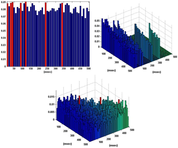
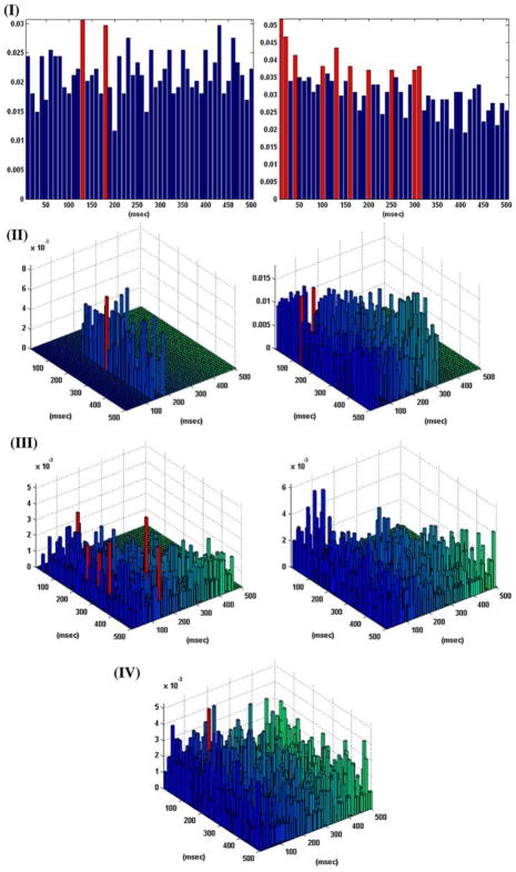
Figure 7 shows the obtained B–V kernels for a two-input/one-output case of the other behavioral task (“nonmatch”). Again, the computed CIs do not exhibit any strong patterns of theta rhythmic activity, but exhibit a regular pattern consistent with the alpha rhythm, with inter-lag distances of 80–120 ms, corresponding to frequencies of 8–12 Hz. There is no clear pattern in the sparse active lags selected in the second order B–V kernels of this case. Also, no inhibitory lags were selected in this case by the ranking algorithm.

FIGURE 7.

The computed CIs of the two first order excitatory B–V kernels (I), the two first order inhibitory B–V kernels (II), the second order B–V self-kernels (III), and the second order B–V cross-kernel (IV) for the two-input/one-output case corresponding to a “sample” behavioral task, along with the active lags of the B–V kernels selected by the ranking method (marked with red).

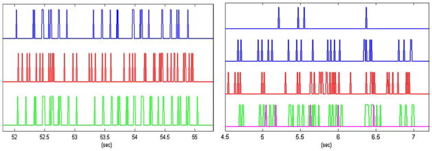
Figure 8 shows representative traces of model predictions, along with the respective inputs and outputs, for a one-input case and a two-inputs case. The presence of a relatively high number of false-positives is evident (especially in the two-input case) that is due to the selected value of the weighting coefficient p. If a higher p-value is selected (not based on the ratio of the input/output mean firing rates), then the number of false positives is reduced, but so does the number of true positives. The proper selection of the p-value remains an open question for future research, as discussed in the final section.

FIGURE 8.

Representative input (blue) and output (red) experimental data, along with the respective model predictions (green) for the single-input “sample task” model (left) shown in Fig. 2 and for the two-input “nonmatch task” model (right) shown in Fig. 7. For the latter case, the predicted output spikes due to the second order kernels are shown in purple.

Table 1 summarizes the modeling results in terms of prediction performance quantified by the TPF and FPF measures (based on 50% estimation data and 50% validation data in each case) for all 13 one-input cases analyzed in this study. The results show that the modeling performance in most of the cases is comparable and close to the average TPF and FPF values of about 55 and 8%, respectively, even though the mean firing rates (MFRs) of the inputs and outputs vary considerably.

TABLE 1.

Summary of modeling performance for the 13 one-input, one-output cases analyzed.

Cases/BE	MFRinput (sp/s)	MFRoutput (sp/s)	r-Value	Data length (s)	TP (%)/FP (%)
#1/Sample	7.07	7.17	0.99	180	46/6.3
#2/Nonmatch	14.99	12.99	1.15	96	30.5/3.5
#3/Sample	16.56	18.69	0.89	136	60/5.3
#4/Nonmatch	4.15	15.23	0.27	124	62.2/9.7
#5/Nonmatch	6.33	15.23	0.42	124	69.4/10.8
#6/Nonmatch	2.6	15.23	0.17	124	40/5.5
#7/Sample	8.69	14.64	0.59	120	81.1/14.2
#8/Sample	2.97	14.64	0.2	120	54.7/8.4
#9/Nonmatch	0.76	15.53	0.05	124	25/2.6
#10/Nonmatch	5.83	15.53	0.38	124	63.5/8.7
#11/Nonmatch	6.33	15.53	0.41	124	74.3/11.8
#12/Sample	1.62	8.73	0.19	108	51.6/10.9
#13/Sample	2.22	8.73	0.26	108	53.1/8.2

Table 2 summarizes the modeling results in terms of prediction errors for the four two-input cases analyzed in this study. The average TPF is about 70%, while the average FPF is about 10% in the two-input case.

TABLE 2.

Summary of modeling performance for the 5 two-input, one-output cases analyzed.

Cases/BE	MFRinput (sp/s)	MFRoutput (sp/s)	r-Value	Data length (s)	TP (%)/FP (%)
#1/Nonmatch	4.15 6.33	15.23	0.69	124	67.6/11.1
#2/Sample	1.62 2.22	8.73	0.44	108	57.1/6.5
#3/Nonmatch	0.76 6.33	15.53	0.46	124	76.7/12.2
#4/Sample	8.69 2.97	14.64	0.8	120	78.8/12.5

As indicated in Part I, this modeling approach can be extended to the auto-regressive case (i.e., when we wish to analyze the internal dynamics of a single point-process in terms of possible underlying temporal patterns). To achieve this, we consider the present value of the single process as the putative “output” and we model its causal relationship with the past epoch of values of the process as the putative “input”. The resulting B–V model is a quantitative representation of the internal dynamics of the point-process and captures all temporal patterns and spectral characteristics of the process. In this pilot application, the auto-regressive modeling approach can be used to discern and quantify possible “neural rhythms” in the data, because an active lag (AL) at lag R of the auto-regressive first order B–V kernel represents a periodic sequence in the data with period R. Two such ALs at distinct lags R1 and R2 represent two periodic sequences in the data with periods R1 and R2, and so on.

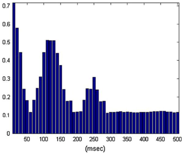
For instance, we may apply it to the input dataset of the first two cases (corresponding to the “sample” behavioral task) to detect the “theta rhythm” that is evident in the CIs of the respective B–V kernels. The results show that the auto-regressive B–V model in the first case has a single AL in the first order excitatory B–V kernel and, in the second case, it has a single AL in the second order B–V kernel, as shown in Fig. 9. In both cases the location of the AL is consistent with the periodicity of the theta rhythm (i.e., 7–8 Hz). No inhibitory ALs were identified in these cases. We should make the clear distinction between the internal dynamics of the input process (described by the auto-regressive B–V kernels) and the causal dynamics of the input–output relation (described by the input–output B–V model).

FIGURE 9.

The auto-regressive B–V models of the input point-processes in the first two one-input cases that contain the theta rhythm. In the first case, only a single AL was identified in the first order excitatory B–V kernel and, in the second case, only a single AL in the second order B–V kernel. The location of the selected ALs corresponds to the periodicity of the theta rhythm. The difference between the two cases seems to be the amount of broadband background activity.

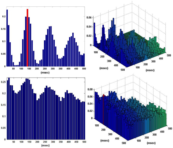
We should also note that a B–V kernel with a periodic structure in its ALs will generate an output with the rhythm depicted in this B–V kernel even when its input has no such internal rhythm. This important fact is akin to “band-pass filtering” in a point-process context, and it is demonstrated in Fig. 10, where we show the CI values of the auto-regressive B–V kernel of the output process generated by a first order B–V kernel with two ALs at lags that have a distance equal to the period of the theta rhythm, in response to a Poisson input process. Since the latter is a random point-process with no temporal patterns by construction, the “band-pass” operation of this B–V kernel is evident in the periodic structure of the computed CI values.

FIGURE 10.

The computed CI values of the “auto-regressive kernel” of the output of a system defined by a first order B–V kernel with two ALs at lags that have a distance equal to the period of the theta rhythm in response to a Poisson input process. The periodic structure of these CI values demonstrates the “band-pass” operation performed by this B–V kernel.

DISCUSSION

The purpose of this paper is to demonstrate the feasibility of the new Boolean–Volterra modeling approach to neural systems with point-process inputs and outputs (presented in the companion paper) through a pilot application to the CA3-to-CA1 mapping of neuronal activity in the rat hippocampus during two behavioral tasks. The presented results demonstrate the potential capabilities of the proposed approach and hold the promise of providing some novel insights into the functional characteristics of this neuronal system through proper interpretation of the obtained Boolean–Volterra (B–V) kernels. This “proper” interpretation of the B–V kernels concerns the patterns of their “active lags” and remains an open issue for future research. An initial interpretation of the B–V kernels obtained in this study is presented here in order to commence this process of discovery and point out some key strengths of the proposed approach.

Let’s start with the first example of the one-input case for a “sample” behavioral task that is shown in Fig. 2. The periodic pattern in the computed CIs of the first order and second order B–V kernels (with a period of about 140 ms) corresponds to the “theta rhythm” of about 7–8 Hz that has been previously observed in studies of the rat hippocampus^7,17,24 and in studies of hippocampal EEG in behaving rats.⁵ This rhythmic activity is present in the input data in this case and does not result from the action of this particular neuron (i.e., it is not related to its dynamics). On the contrary, this particular neuron seems to perform an operation akin to “stop-band filtering” of the theta rhythm present in the input through the active lags of the inhibitory B–V kernel which are located at the 13th and 14th lags (i.e., they prevent the firing of a spike 130–140 ms after the appearance of an input spike). Note that each lag is 10 ms and the first order excitatory B–V kernel of this neuron has a simple relay characteristic (i.e., it generates an output spike with a latency of about 10 ms in response to each input spike, unless it is blocked by the inhibitory kernel). It is evident that this inhibitory/filtering operation blocks every other output spike driven by the theta rhythm of the input and doubles the period of the rhythm at the output of the neuron. Thus the resulting output rhythm has half the theta frequency (i.e., 3.5–4 Hz).

In the second example of the one-input case for a “sample” behavioral task that is shown in Fig. 3, the location of the single active lag (AL) of the inhibitory kernel (on the third lag) indicates that this kernel performs a refractory operation for about 10 ms following the firing of an output spike with a latency of 20 ms after each input spike due to the relay action of the single AL in the first order excitatory kernel (located on the second lag). Note that this neuron also has an AL in its second order kernel at lag coordinates 1 and 3, which indicates that a spike will be fired when the neuron receives a pair of spikes one lag apart. Clearly, this neuron will neither generate nor block/filter a possible theta rhythm in its input.

In the third example of the one-input case for a “nonmatch” behavioral task that is shown in Fig. 4, there are multiple ALs in the first order excitatory kernel that form a complex pattern and may generally indicate the presence of rhythms in the input-output dynamics. For instance, a inter-lag distance of 20–30 ms between selected ALs may reflect the presence of the “gamma rhythm” (30–50 Hz) in the system dynamics, or a distance of 80–120 ms between selected ALs may reflect the presence of the “alpha rhythm” (~8–12 Hz). Such inter-lag distances are actually seen in the multiple ALs of this first order B–V kernel. Such an important claim will require more extensive evidence and repeated analysis that is expected to take place in the near future. What is also worth further discussion is the functional implication of the three ALs selected in the second order B–V kernel of this “nonmatch” task. The locations of these ALs may generally allow “detection” of the presence and/or interactions between different rhythms in the input. For instance, consider only a single second order AL with lag-coordinates i and j (i.e., no other ALs or B–V kernels exist in the model of this neuron). This will give rise to an output spike (with latency the maximum of i and j) when the neuron receives a pair of input spikes separated by T1 ms equal to |i − j| lags. Therefore, a periodic input sequence with period T2 will generate at the output another periodic sequence if and only if T1 and T2 are equal or multiples of each other. This represents an operation akin to band-pass filtering in the context of point-processes (although broader in scope, since it allows harmonics and sub-harmonics as well). One may extend these notions to the case of multiple ALs in the second order B–V kernel and in combination with first order dynamics (both excitatory and inhibitory) to begin to get a sense of how flexible and powerful this modeling/analysis tool can be in representing complex behavior of neuronal ensembles, when properly deployed. This may prove useful in systems of high functional complexity, like the functional connectivity between the CA3 and CA1 regions of the hippocampus which is influenced by spatially selective activity and place encoding¹⁹ as well as episodic memory encoding.¹⁴

Similar interpretation of the obtained B–V kernels can be applied to the two-input cases, where the complexity of the model is further increased by the joint consideration of two input sequences and the possible presence of B–V cross-kernels that account for interactions between the inputs as they reflect on the output of the neuron. Consider, for instance, a neuron that has only one cross-kernel AL at lag-coordinates L1 (relative to input 1) and L2 (relative to input 2). This neuron will fire periodically every L lags, where L = max(L1, L2), if and only if the input 1 has a periodicity of period L1 and the input 2 has a periodicity of period L2. Thus the periodic activity of this neuron can “detect” the joint presence of the two rhythms (L1 and L2) in the two inputs. One may extend this concept to multiple inputs and rhythms.

The predictive capability of the obtained B–V models was evaluated by means of the true-positive (TP) and false-positive (FP) predictions of output spikes. The results for all 13 cases examined in this study are reported in Table 1. Most cases are close to the average TP and FP fractions of about 55 and 8%, respectively. The assessment of this predictive performance depends on the relative weighting of TP vs. FP predictions that is regulated through the parameter r that is the power to which we raise the ratio TPF/FPF of the TP and FP fractions in order to evaluate the figure of merit Q (see Part I). Although the value of the parameter r was set equal to the ratio of the input/output mean firing rates in this study (as a reasonable choice for balancing disparities between the two firing rates), its proper selection remains an open question for future research. If the FPF is deemed high relative to the TPF (as it may appear, especially in the two-input cases), then a higher p-value can be selected that will reduce the number of false positives—although it will also reduce the number of true positives. Also it should be noted that multiple unaccounted inputs, and other ambient factors, are likely to exist in a realistic case and are bound to prevent the achievement of high TPF values for the predicted output of a multi-input neuron when the employed model utilizes only a few of its actual inputs.

An interesting result was obtained in the auto-regressive modeling of the input point-processes in the first two one-input cases that contain the theta rhythm (see Fig. 9). A single AL was identified in both cases, with a location consistent the periodicity of the theta rhythm. However, this single AL was identified in the first order excitatory B–V kernel in the first case, but in the second order B–V kernel in the second case. Although both account for the theta rhythm, there is an obvious difference between the two models which seems to be due to the respective broadband background activity. Specifically, the second case has a higher random/broadband background activity and seems to require the second order operation of checking the joint presence of two spikes (at the proper lags) to discern the theta rhythm from the random background.

Finally, the question naturally arises as to how the proposed B–V modeling approach compares with existing nonlinear modeling methods that have been used in the same context, such as the “regular” Volterra modeling used extensively by our group for the same purpose (see, for instance, Berger et al.,³ Dimoka et al.,⁶ Gholmieh et al.,¹¹ Marmarelis,¹⁶ and Zanos et al.,^25,26). Using the first and second order Volterra kernels in the first example, we obtain comparable TPF values (51 vs. 46%) for the same FPF value (6.3%). However, the required computational time was about half in the B–V approach, and the number of kernel values that are needed to define the two models is vastly smaller in the B–V case. Both of these facts can be important in a practical context, especially when this modeling approach is applied to multi-unit neuronal ensembles.

These initial results demonstrate the potential capabilities of the proposed modeling approach for neural systems with point-process inputs and outputs. However, further corroboration by additional data is required, as well as further exploration of many aspects of the new approach (including the functional and physiological interpretation of the obtained models) before it can become widely accepted by the peer community and be used for advancing our understanding of neuronal function.

References

- 1.Berger TW, Ahuja A, Courellis SH, Deadwyler SA, Erinjippurath G, Gerhardt GA, Gholmeih G, Granacki JJ, Hampson RE, Hsiao M-C, LaCoss J, Marmarelis VZ, Nasiatka P, Srinivasan V, Song D, Tanguay AR, Jr, Wills J. Hippocampal-cortical neural prostheses to restore lost cognitive function. IEEE EMBS Special Issue: Toward Biomimetic Microelectron. Neural Prostheses. 2005;24:30–44. doi: 10.1109/memb.2005.1511498. [DOI] [PubMed] [Google Scholar]
- 2.Berger TW, Baudry M, Brinton RD, Liaw JS, Marmarelis VZ, Park AY, Sheu BJ, Tanguay AR. Brain-implantable biomimetic electronics as the next era in neural prosthetics. Proc IEE. 2001;89:993–1012. [Google Scholar]
- 3.Berger TW, Eriksson JL, Ciarolla DA, Sclabassi RJ. Nonlinear systems analysis of the hippocampal perforant path-dentate system. II. Effects of random train stimulation. J Neurophysiol. 1988;60:1077–1094. doi: 10.1152/jn.1988.60.3.1077. [DOI] [PubMed] [Google Scholar]
- 4.Berger TW, Glanzman DL. Towards Replacement Parts for the Brain: Implantable Biomimetic Electronics as Neural Prostheses. Chapter 12. Cambridge, MA: MIT Press; 2005. p. 241. [Google Scholar]
- 5.Buzsaki G, Leung LW, Vanderwolf CH. Cellular bases of hippocampal EEG in the behaving rat. Brain Res. 1983;287(2):139–171. doi: 10.1016/0165-0173(83)90037-1. [DOI] [PubMed] [Google Scholar]
- 6.Dimoka A, Courellis SH, Gholmieh G, Marmarelis VZ, Berger TW. Modeling the nonlinear properties of the in vitro hippocampal perforant path-dentate system using multi-electrode array technology. IEEE Trans Biomed Eng. 2008 doi: 10.1109/TBME.2007.908075. (in press) [DOI] [PMC free article] [PubMed] [Google Scholar]
- 7.Foster DJ, Wilson MA. Hippocampal theta sequences. Hippocampus. 2007;17:1093–1099. doi: 10.1002/hipo.20345. [DOI] [PubMed] [Google Scholar]
- 8.Gholmieh G, Courellis SH, Fakheri S, Cheung E, Marmarelis VZ, Baudry M, Berger TW. Detection and classification of neurotoxins using a novel short-termplasticity quantification method. Biosens Bioelectron. 2003;18(12):1467–1478. doi: 10.1016/S0956-5663(03)00120-9. [DOI] [PubMed] [Google Scholar]
- 9.Gholmieh G, Courellis SH, Marmarelis VZ, Berger TW. An efficient method for studying short-term plasticity with random impulse train stimuli. J Neurosci Methods. 2002;21(2):111–127. doi: 10.1016/S0165-0270(02) 00164-4. [DOI] [PubMed] [Google Scholar]
- 10.Gholmieh G, Courellis SH, Marmarelis VZ, Berger TW. Detecting CA1 short-term plasticity variations with changes in stimulus intensity and extracellular medium composition. Neurocomputing. 2005;63:465–481. doi: 10.1016/j.neucom.2004.07.001. [DOI] [Google Scholar]
- 11.Gholmieh G, Courellis SH, Marmarelis VZ, Berger TW. Nonlinear dynamic model of CA1 short-term plasticity using random impulse train stimulation. Ann Biomed Eng. 2007;35(5):847–857. doi: 10.1007/s10439-007-9253-6. [DOI] [PubMed] [Google Scholar]
- 12.Gruart A, Munoz MD, Delgado-Garcia JM. Involvement of the CA3-CA1 synapse in the acquisition of associative learning in behavingmice. JNeurosci. 2006;26(4):1077–1087. doi: 10.1523/JNEUROSCI.2834-05.2006. [DOI] [PMC free article] [PubMed] [Google Scholar]
- 13.Hampson RE, Simeral JD, Deadwyler SA. Distribution of spatial and nonspatial information in dorsal hippocampus. Nature. 1999;402(6762):610–614. doi: 10.1038/45154. [DOI] [PubMed] [Google Scholar]
- 14.Leutgeb S, Leutgeb JK, Moser MB, Moser EI. Place cells, spatial maps and the population code for memory. Curr Opin Neurobiol. 2005;15(6):738–746. doi: 10.1016/j.conb.2005.10.002. [DOI] [PubMed] [Google Scholar]
- 15.Levy WB. A sequence predicting CA3 is a flexible associator that learns and uses context to solve hippocampal-like tasks. Hippocampus. 1996;6(6):579–590. doi: 10.1002/(SICI)1098-1063(1996)6:6<579::AID-HIPO3>3.0.CO;2-C. [DOI] [PubMed] [Google Scholar]
- 16.Marmarelis VZ. Nonlinear Dynamic Modeling of Physiological Systems. New York: Wiley; 2004. p. 359. [Google Scholar]
- 17.Maurer AP, MacNaughton BL. Network and intrinsic cellular mechanisms underlying theta phase precession of hippocampal neurons. Trends Neurosci. 2007;30(7):325–333. doi: 10.1016/j.tins.2007.05.002. [DOI] [PubMed] [Google Scholar]
- 18.Menschik ED, Yen SC, Finkel LH. Model- and scale-independent performance of a hippocampal CA3 network architecture. Neurocomputing. 1999;26–27:443–453. doi: 10.1016/S0925-2312(99)00050-8. [DOI] [Google Scholar]
- 19.O’Keefe J, Dostrovsky J. The hippocampus as a spatial map. Preliminary evidence from unit activity in the freely-moving rat. Brain Res. 1971;34(1):171–175. doi: 10.1016/0006-8993(71)90358-1. [DOI] [PubMed] [Google Scholar]
- 20.Sargsyan A, Melkonyan A, Mkrtchian H, Paptheodoropoulos C, Kostopoulos G. A computer model of field potential responses for the study of short-term plasticity in hippocampus. J Neurosci Methods. 2004;135(1–2):175–191. doi: 10.1016/j.jneumeth.2003.12.009. [DOI] [PubMed] [Google Scholar]
- 21.Song D, Chan RH, Marmarelis VZ, Hampson RE, Deadwyler SA, Berger TW. Nonlinear dynamic modeling of spike train transformations for hippocampal-cortical prostheses. IEEE Trans Biomed Eng. 2007;54(6):1053–1066. doi: 10.1109/TBME.2007.891948. [DOI] [PubMed] [Google Scholar]
- 22.Touretzky DS, Redish AD. Theory of rodent navigation based on interacting representations of space. Hippocampus. 1996;6(3):247–270. doi: 10.1002/(SICI)1098-1063(1996)6:3<247::AID-HIPO4>3.0.CO;2-K. [DOI] [PubMed] [Google Scholar]
- 23.Treves A, Rolls ET. Computational constraints suggest the need for two distinct input systems to the hippocampal CA3 network. Hippocampus. 1992;2(2):189–199. doi: 10.1002/hipo.450020209. [DOI] [PubMed] [Google Scholar]
- 24.Vertes RP. Hippocampal theta rhythm: a tag for short-term memory. Hippocampus. 2005;15(7):923–935. doi: 10.1002/hipo.20118. [DOI] [PubMed] [Google Scholar]
- 25.Zanos TP, Courellis SH, Berger TW, Hampson RE, Deadwyler SA, Marmarelis VZ. Nonlinear modeling of causal interrelationships in neuronal ensembles. IEEE Trans Neural Syst Rehabil Eng. 2008;16(4):336–352. doi: 10.1109/TNSRE.2008.926716. [DOI] [PMC free article] [PubMed] [Google Scholar]
- 26.Zanos TP, Courellis SH, Hampson RE, Deadwyler SA, Marmarelis VZ, Berger TW. A multi-input modeling approach to quantify hippocampal non-linear dynamic transformations. IEEE Eng Med Biol Conf. 2006;1:4967–4970. doi: 10.1109/IEMBS.2006.260575. [DOI] [PubMed] [Google Scholar]