Controlled Experimental Study Depicting Moving Objects in View-Shared Time-Resolved 3D MRA

Abstract

Various methods have been used for time-resolved contrast-enhanced MRA (CE-MRA), many involving view sharing. However, the extent to which the resultant image time series represents the actual dynamic behavior of the contrast bolus is not always clear. Although numerical simulations can be used to estimate performance, an experimental study can allow more realistic characterization. The purpose of this work was to use a computer-controlled motion phantom for study of the temporal fidelity of 3D time-resolved sequences in depicting a contrast bolus. It is hypothesized that the view order of the acquisition and the selection of views in the reconstruction can affect the positional accuracy and sharpness of the leading edge of the bolus and artifactual signal preceding the edge. Phantom studies were performed using dilute gadolinium-filled vials that were moved along tabletop tracks by a computer-controlled motor. Several view orders were tested, which use view-sharing and Cartesian sampling. Compactness of measuring the k-space center, consistency of view ordering within each reconstruction frame, and sampling the k-space center near the end of the temporal footprint were shown to be important in accurate portrayal of the leading edge of the bolus. A number of findings were confirmed in an in vivo CE-MRA study.

INTRODUCTION

Contrast enhanced magnetic resonance angiography (CE-MRA) is a noninvasive technique that is widely used for the diagnosis of vascular disease (1–3). Technical challenges in CE-MRA have included imaging the arterial phase of the contrast bolus without venous contamination (4) and obtaining images with adequately high spatial resolution. Also, CE-MRA methods can possibly be prone to artifacts due to the motion of flowing blood, the varying concentration of contrast material, and the manner in which k-space is acquired (4,5). The issue of timing the data acquisition to the arterial phase has been addressed with a variety of techniques such as a test bolus (6) or automated triggering (7,8). Also, centric view orders (9,10) if initiated effectively can allow extended acquisition times, and thus high spatial resolution arterial-phase images without appreciable venous signal. Alternatively, time-resolved MRA allows matching the central k-space sampling to peak arterial enhancement by repeatedly acquiring images as contrast material moves through the area of interest, either with 2D (11,12) or 3D (13) acquisition. However, due to the extended (typically tens of seconds) dwell time of intravenously injected contrast material in the vasculature, this generally involves a tradeoff: time spent in resampling low spatial frequencies for improved temporal resolution could have been spent in sampling high spatial frequencies for improved spatial resolution (14). This in turn has been addressed by attempting to speed up the acquisition with short repetition times or by using view sharing (13,15,16), a method by which images are reconstructed more frequently than the intrinsic image acquisition time.

Recently the tradeoff of time with spatial resolution in time-resolved sequences has been changed with the advent of parallel acquisition techniques (17–19). This is particularly true when 2D techniques (20) are applied to 3D imaging, as is typically the case for CE-MRA. In this application accelerations of four or higher can routinely be obtained (21–24). Along with parallel acquisition there has been recent development in k-space sampling and reconstruction strategies for 3D time-resolved imaging (13,16,23,25,26). These parallel acquisition and sampling methods have collectively allowed high resolution (near 1 mm isotropic) 3D image sets to be generated at a higher rate than commonly done previously.

In spite of the increased frame rate of 3D data sets, it is not always clear to what extent the resultant image time series truly represents the dynamic behavior of the object of interest. Although simulations can be used to estimate various aspects of performance (4,5,25,27–29), an experimental study can allow characterization under actual conditions of acquisition. The purpose of this work was to develop a computer-controlled motion phantom, simulating bolus travel, for study of the fidelity of 3D time-resolved sequences. The phantom studies allow determination of the accuracy in portraying a rapid influx of contrast material into a vessel and the linear passage of a contrast bolus across an extended FOV. Accelerated MR acquisition coupled with precise control of the phantom motion permit extension of subjective evaluation criteria (e.g. ghosting and blurring) to quantitative assessment of the sharpness of the bolus leading edge (longitudinal resolution), absolute accuracy in portraying position and velocity, and extent of any artifact ahead of (“anticipation”) or behind (“persistence”) the bolus. Understanding these features may be beneficial for understanding overall temporal fidelity, pulse sequence design, and quantitative use of contrast bolus arrival time information. Specific hypotheses are described in which we assess the effects of centricity of views, temporal compactness in sampling the center of k-space, consistency of views from frame to frame, extent of temporal footprint, and reconstruction data selection on image fidelity in view-shared time-resolved 3D MRA. Several of the properties are illustrated in an in vivo CE-MRA study.

METHODS

Experimental Setup

Studies were performed using two dilute gadolinium-filled vials (400 mm long, circular cross section with 22 mm inner diameter) that were moved along tabletop tracks by a computer-controlled motor (Fig. 1). Each vial was connected to a toothed rod that was driven using a stepper motor (0.1 mm/step), which provided precise control and reproducibility of motion. A computer program designated a start position for the rods and a travel velocity. For each experiment, the motion of the vials was automatically triggered with the initiation of the pulse sequence. A water phantom was placed in the center of the FOV to provide increased signal for calibration. Unless indicated otherwise, the (x,y,z) axes used were those shown in Fig. 1 with × (frequency) in and out of the scanner bore along the tabletop. This definition of axes matches the typical coronal orientation used in 3D CE-MRA of the lower legs with frequency encoding along the S/I direction, and thus the motion studied mimics that of the contrast bolus advancing along the major vessels of the calves. In several experiments the axes were swapped so as to study motion along one of the phase encoding directions.

Figure 1.

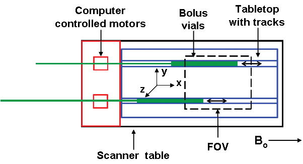
Experimental setup for phantom studies. Dilute gadolinium-filled “bolus” vials were moved along tabletop tracks by a computer controlled motor, which designates a start position and travel velocity.

Phase Encoding View Orders

Fig. 2 shows three view orders that were used in our experimental studies: (a,b) Cartesian Acquisition with Projection-Reconstruction-like sampling (CAPR) (23), (c,d) Centric k_Y-k_Z, and (e,f) Centric k_Y. Each is a 3DFT acquisition using Cartesian sampling in k_Y-k_Z space; phase encoding is performed along the k_Y and k_Z axes and echoes are read out along k_X. Each view order implements view-sharing in which a central region of k-space plus one portion of the periphery is sampled each update. For all cases and throughout this work, the central region is denoted in orange. CAPR is described in detail in Ref. (23), but briefly, the sampling pattern consists of a central circular region in k_Y-k_Z space which is sampled every image update (Fig. 2a). The annular region beyond this is divided into N groups of vanes, one of which is sampled every update. For this work N = 4 was routinely used. The vane pattern allows 2D partial Fourier acquisition (30) and this was used. Two time orders of sampling were studied. For the elliptical centric (EC) order the sampling starts at the origin, covers the central region and one vane set. For the reverse EC order (REC) this time order is reversed. The Centric k_Y-k_Z order samples a center circle each image update, and the outer region is divided into N concentric annuli of equal area (Fig. 2c). The Centric k_Y order sequentially samples a rectangle centered in k_Y that spans all desired k_Z phase encodes each image update. The outer region is composed of N groups of two similar rectangles on either side of the origin that consecutively increase in distance from the k_Y center (Fig. 2e). The view orders were generated such that the image update times were comparable but the degree of view sharing and the temporal footprint varied according to how many image updates were required to fill k-space for each sampling method. These k-space patterns were chosen to have equivalent acquired spatial resolution. The number of central k-space points was equal for all view orders and was determined by optimizing SNR and temporal resolution for the application. The areas of the peripheral regions were not constrained to match that of the central orange regions. With the incorporation of 2D SENSE to the CAPR view order the number of central points was kept constant.

Figure 2.

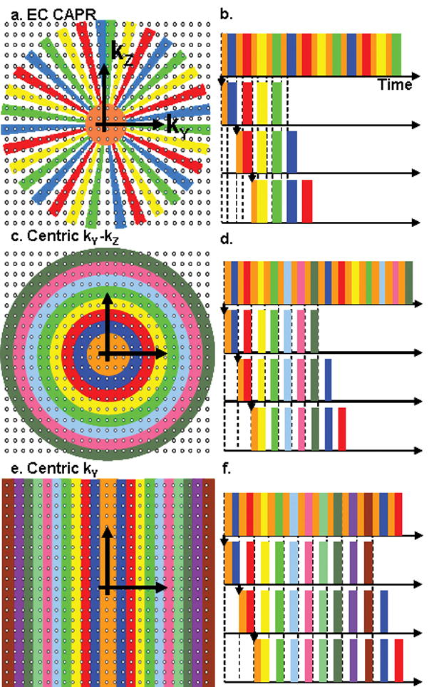
Illustration of k_Y-k_Z sampling patterns and temporal ordering for view orders. (a,b) EC CAPR. Sampling consists of a central circular region (orange) and a peripheral region apportioned into N vane sets. Here N is set to 4. (c,d) Centric k_Y-k_Z. k-space is apportioned into a central circle (orange) and N concentric annuli. (e,f) Centric k_Y. k-space is apportioned into a central rectangle (orange) and N rectangles centered about the k_Y axis. For each view order the center and one section of the periphery are acquired each image update (b,d,f).

Previously a randomized view order has been shown to provide certain advantages in 2D time-resolved imaging (31), and here we considered such an ordering for 3D. Specifically, the identical set of points in the k_Y-k_Z plane was sampled as for N = 4 EC CAPR, but the ordering of views within a single update period was randomized. That is, in any one update interval, the points in central k-space and the vane set to be updated were first identified, but these were next sampled randomly rather than in the EC manner. The process was repeated for each subsequent update.

Data Selection for Reconstruction

When some phase encoding views or k-space points are sampled more frequently than others, there can be a choice as to which measurement of a redundantly sampled view should be incorporated into the reconstruction. This is illustrated in Fig. 3 for the CAPR sequence where the k-space center is sampled four times more frequently than the periphery. Assume for the time being that only one k-space center is incorporated into any reconstruction, and averaging or temporal interpolation is not done. Then, from the playout of views shown in (a), the data can be selected in several different ways as input to the reconstruction. Define the “reconstruction delay” as the number of central samplings acquired after the k-space center used for a given reconstruction. A Delay N-1 reconstruction (Fig. 3b, where here N-1 = 3) uses the earliest acquired center for a given full peripheral k-space sampling. A Delay N-2 reconstruction (Fig. 3c) uses the next earliest. A Delay 0 reconstruction (Fig. 3d) uses the most recently acquired center for a given full peripheral k-space sampling and is the default method for our studies. A Delay −1 reconstruction for an EC sampling pattern (Fig. 3e) is defined as one using the most recently acquired center but not the subsequent sampling of peripheral k-space; rather, the four vane sets acquired prior to that center are used.

Figure 3.

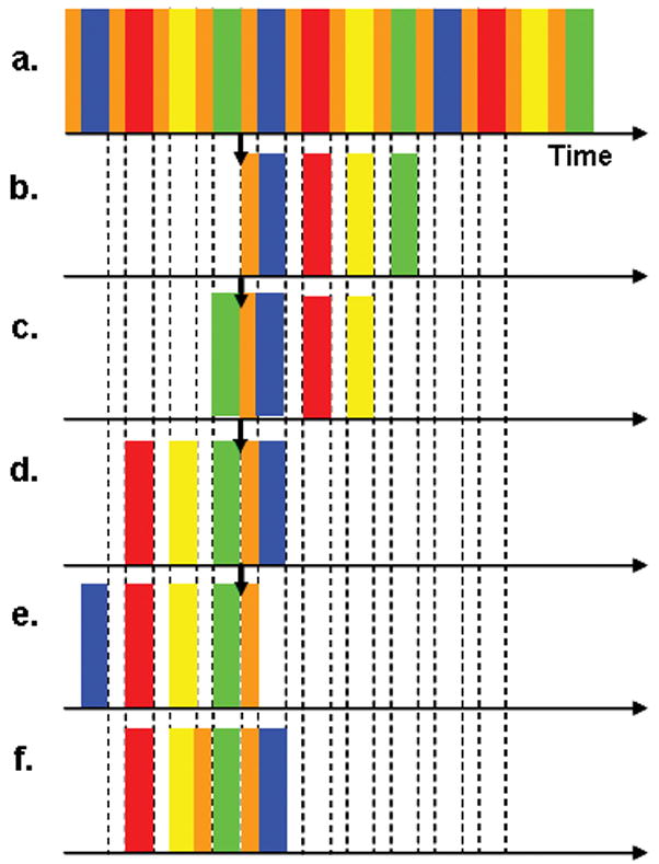
Schematic of playout of all views for an EC CAPR (N = 4) acquisition (a) and the selection of data for reconstruction Delay 3 (N-1) (b), Delay 2 (c), Delay 0 (d), Delay −1 (e), and Delay 0 averaging two centers (f). Corresponding frames are constructed using the same center regardless of delay while the high pass views used for a reconstruction are altered. Delay 0 uses the most recently acquired center while Delay N-1 uses the earliest acquired center over a full peripheral k-space sampling.

In additional experiments the effects of averaging multiple samplings of central k-space were studied. Using the Delay 0 sort as a starting point (Fig. 3d), the previous one, two, and three central samplings were averaged with the original central sampling. In all cases only one sampling of each of the four vane sets was used for reconstruction. The sort used with one previous central sampling (for a total of two) is illustrated in Fig. 3f.

Specific Hypotheses

Several specific hypotheses were studied. First, we hypothesize that view orders that are centric in both k_Y and k_Z and thus with compact sampling of the center of k-space provide a sharper bolus leading edge than view orders which are not. Second, we hypothesize that view orders that sample each spatial frequency at a constant time interval (consistent sampling of k-space in time) provide accurate portrayal of continuous linear motion. Third, we hypothesize that the higher temporal resolution and shorter temporal footprint achieved by the application of 2D SENSE will improve depiction of the bolus leading edge. Finally, we hypothesize that a reconstruction of Delay 0 decreases the extent of the anticipation artifact in comparison to a reconstruction of longer delay.

Experiments Performed

Experiments were run at 3.0T (GE Medical Systems V14.0) using a 3D fast spoiled gradient echo sequence with scan parameters: TR/TE = 6.3/2.8 ms, flip angle = 30°, BW = ± 62.5 kHz, FOV 40 cm (S/I frequency) × 32 cm (R/L phase) × 13.2 cm (A/P slice), sampling matrix 400 (S/I) × 320 (R/L) × 132 (A/P), 1 mm isotropic resolution. These parameters substantially match those used for CE-MRA at our institution (32). In specified acquisitions 2D SENSE was performed in which case the acceleration along z was fixed at R_Z = 2 and the acceleration R_Y along y chosen to provide the desired net acceleration R = R_Y*R_Z. The calibration scan for SENSE was a 3D fast spoiled gradient echo sequence with TR/TE = 6.7/4.2 ms, flip angle = 10°, FOV = 40 cm, BW = ± 31.25 kHz, sampling matrix 400 × 160 × 132. A high resolution calibration scan was used for improved performance of the SENSE reconstruction. The coil used was an eight-element linear array (1×8), with an element length of 22 cm, designed for imaging the peripheral vasculature of the lower legs (33), placed circumferentially around the phantom.

The specific hypotheses were studied in a series of experiments. To compare REC CAPR, EC CAPR, Centric k_Y-k_Z, and Centric k_Y view orders, each was used to acquire time-resolved images as the vials in the above design were moved through one FOV (40 cm) at a bolus speed of 4 mm/s. The view orders were also studied with the application of 2D SENSE at a bolus speed of 16 mm/s. These velocities are toward the lower end of the range of those encountered in vivo in CE-MRA of the calves (34) and also allow multiple image updates as the phantom traverses the FOV. To study the effect of motion along the phase encoding direction on leading edge artifact, the phase and frequency encoding axes were swapped and images were acquired using the EC CAPR view order. To study the effects of parallel imaging on performance, we compared EC CAPR acquisitions with SENSE accelerations of R = 1, 2, 4, and 7.3 at a bolus speed of 8 mm/s. To assess the importance in sampling central k-space in a temporally compact manner versus randomized sampling done over the entire image update time, the standard EC CAPR and randomly ordered CAPR sequences were used to acquire images with R = 1 (no SENSE acceleration) and R = 7.3 at a bolus speed of 4 mm/s. The effect of temporal averaging on depiction of the bolus leading edge was studied by reconstructing an EC CAPR (N = 4) acquisition phantom study and an in vivo lower leg contrast-enhanced study with averaging of one, two, three, and four k-space centers. The effect of reconstruction delay on image quality and motion artifacts was studied by reconstructing the same phantom and in vivo studies as above with Delays of 3 through −1. The in vivo study was approved by the institutional review board, and written consent was obtained from the volunteer subject. It was acquired using the same pulse sequence as above but with R = 8, update time = 4.9 s, and temporal footprint = 19.6 s.

Image Analysis

The images were generally viewed and analyzed as maximum intensity projections (MIPs) along the z direction. The analysis was also performed on central slices from the volume, and the results were in general consistent with those from the MIPs.

The images from the motion phantom studies were analyzed to assess the sharpness and positional accuracy of the bolus leading edge and the accuracy in portraying continuous linear motion. To assess the sharpness of the bolus leading edge, longitudinal line profiles were taken along a five-pixel-wide section of the central axis of the bolus phantom. The temporal frame from which the line profiles were taken was chosen such that the bolus vial was near the center of the FOV in order to minimize the effects of coil signal dropout on leading edge characterization. Lateral line profiles were taken within the central slice in the direction orthogonal to motion at the position along the vessel defined as the leading edge, as described below. Unless stated otherwise the term “line profile” refers to the longitudinal line profile as defined above.

To determine the accuracy of a view order in depicting the bolus position, the bolus leading edge location was found for each image update and compared to the true position of the phantom at that update, which is known from computer control. The bolus leading edge was defined as the position along the axis where the bolus vial signal intensity first reaches 75% of the maximum signal in that frame, when searching from the opposite direction of bolus travel. The true position was defined as the location of the bolus vial when the central-most point in k-space was sampled and was calculated from the bolus velocity and image update time. Static reference images were obtained with the bolus vials fixed at these locations. Positional accuracy was quantified by determining the difference between the position of bolus leading edge measured using the 75% criterion and that in the reference static image. Blurring of the leading edge was quantified by calculating the distance between the bolus leading edge (75% maximum signal) and the position where the leading edge drops to 25% of the maximum bolus signal intensity. The 75% and 25% signal thresholds were chosen as they logically represent the positions at which contrast material has predominantly filled in and not respectively. Also, the 25% level was high enough to distinguish edge blurring from anticipation artifact.

To assess the accuracy of the view orders in depicting continuous linear motion, the distances between the measured leading edge positions from one image update to the next for a given acquisition were compared. Equal spacing between leading edge positions indicates the accurate portrayal of linear motion or constant velocity. This was also studied by plotting the leading edge position versus time for an imaging series. Means and standard deviations were calculated for positional accuracy and leading edge blur by using multiple time frames from multiple acquisitions.

RESULTS

Fig. 4 shows a composite of consecutive frames using three of the four view orders: REC CAPR (b1–b3), EC CAPR (c1–c3) and Centric k_Y (d1–d3) all acquired with the bolus phantom moving left to right at a speed of 16 mm/s and using 2D SENSE (R = 7.3). Images of the static phantom at the corresponding time frames are shown in (a1–a3). For each static image (a1, a2, a3) all views were acquired with the phantom fixed at the true position for the corresponding dynamic cases. For each view order the interval between each image, e.g. b1 to b2 and b2 to b3 is 5.6 s, corresponding to an advancement of the phantom of 89 mm along the x-direction. The k-space sampling pattern over time is matched to longitudinal position and is displayed on the images by the colored blocks, which correspond to those in Fig. 2. The vertical lines mark the calculated true bolus leading edge positions at the times of sampling of the very central-most view. The red arrows indicate the measured positions of the bolus leading edge in each frame as found using the 75% maximum signal intensity algorithm. The distance between a red arrow and the nearby vertical line indicates the error in position estimation. These displacements in the depicted bolus leading edge position are summarized in Table 1 for the different view orders for the above study (R = 7.3 at a bolus velocity of 16 mm/s) as well as for the case of no SENSE acceleration (R = 1) at a bolus velocity of 4 mm/s.

Figure 4.

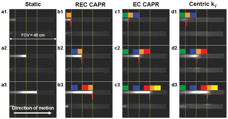
Comparison of accuracy in depiction of bolus leading edge position for different view orders (bolus velocity 16 mm/s). The vertical lines represent the true bolus position as shown in the static images (a1–a3) and at the time of measurement of the central-most view for the other cases (b–d). The red arrows indicate the measured leading edge position for the motion studies.

Table 1.

Quantification of leading edge positional accuracy for view orders. Displacement is defined as the distance between the contrast bolus leading edge, as observed in the image, and the position of the edge at the time of sampling the central-most phase encoding view. A negative (positive) value means that the observed edge of the moving phantom lags (leads) the true position in the direction of motion. The corresponding figures are identified for Case II.

View order	Case I: 4 mm/s, R = 1		Case II: 16 mm/s, R = 7.3
	Displacement mean ± std (mm)	% displacement per update distance (104 mm)	Displacement mean ± std (mm)	% displacement per update distance (89 mm)	Figure
REC CAPR	−7.5±0.6	7.2	−5.5±2.3	6.1	4b
EC CAPR	−1.3±0.5	1.2	−1.9±2.5	2.0	4c
Centric kY-kZ	−1.3±0.5	1.2	−2.3±2.8	2.4	-
Centric kY	25.3±33.3	24.3	12.9±5.5	14.6	4d

Fig. 5 shows enlargements of the leading edge in a selected frame from acquisitions using each the following view orders: (a) REC CAPR, (b) EC CAPR, (c) Centric k_Y-k_Z, and (d) Centric k_Y, all acquired with no SENSE acceleration (R = 1) at a bolus speed of 4 mm/s. Note that the scales on the line profiles vary with the SNR of the images. The REC CAPR image has increased signal at the leading edge due to sampling central k-space at the very end of the image update. The Centric k_Y image has reduced SNR due to dispersion of signal in both longitudinal and lateral artifact. Vertical lines in the images and line profiles mark the 75% maximum signal location (the bolus leading edge) and the 25% maximum signal location. The distance between these lines, defined previously as the leading edge blur, is quantified and displayed on the profiles. Also shown is the image update distance, here 104 mm, which corresponds to the longitudinal distance traversed by the phantom over one image update. Table 2 is a summary of the extent of leading edge blur for the various view orders for the above two cases from Figs. 4 and 5.

Figure 5.

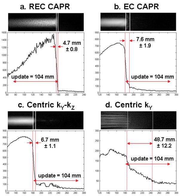
A selected frame from a motion study (bolus velocity 4 mm/s) and the corresponding longitudinal line profiles are shown for the view orders (a) REC CAPR, (b) EC CAPR, (c) Centric k_Y-k_Z, and (d) Centric k_Y. Motion is left to right. The vertical lines mark the 75% and 25% signal positions along the leading edge used to determine the width of the leading edge blur. Also noted is the 104 mm distance the phantom travels during one time frame. REC CAPR shows the sharpest leading edge and Centric k_Y the greatest extent of blur.

Table 2.

Quantification of leading edge blur for view orders. The corresponding figures are identified for Case I.

View order	Case I: 4 mm/s, R = 1			Case II: 16 mm/s, R = 7.3
	Blur mean ± std (mm)	Figure	% blur per update distance (104 mm)	Blur mean ± std (mm)	% blur per update distance (89 mm)
REC CAPR	4.7±0.8	5a	4.5	4.4±1.0	5.0
EC CAPR	7.6±1.9	5b	7.3	16.9±5.6	18.9
Centric kY-kZ	6.7±1.1	5c	6.4	16.6±5.5	18.6
Centric kY	48.7±12.2	5d	46.7	27.4±6.6	30.7

For each view order in Fig. 4 the frame-to-frame distances between red arrows are relatively constant and approximately match the distance between the fiducial lines, thus showing that all view orders accurately portray the phantom velocity Results of additional studies implementing EC CAPR at lower velocities to provide more updates over the FOV are shown in Fig. 6 where the estimated bolus leading edge is plotted versus time for multiple consecutive frames. At each speed, linear motion is well portrayed (R² = 0.99–1.00) and the absolute velocity depicted (slope of lines) matches the prescribed bolus velocity within 3% for all cases. The Centric k_Y-k_Z and Centric k_Y view orders were similarly evaluated and showed comparable results.

Figure 6.

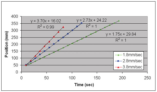
Plot of bolus leading edge position versus time for multiple consecutive time frames implementing EC CAPR at low bolus speeds. The high R² values demonstrate how the consistency of the sampling from frame to frame provides accurate portrayal of linear motion and absolute velocity.

Fig. 7 compares selected image frames and the corresponding longitudinal and lateral line profiles from EC CAPR acquisitions with frequency versus phase encoding performed S/I, along the direction of motion. Results are shown for two cases, no SENSE acceleration (R = 1) with a bolus velocity of 4 mm/s and R_Z = 2 with a bolus velocity of 8 mm/s.

Figure 7.

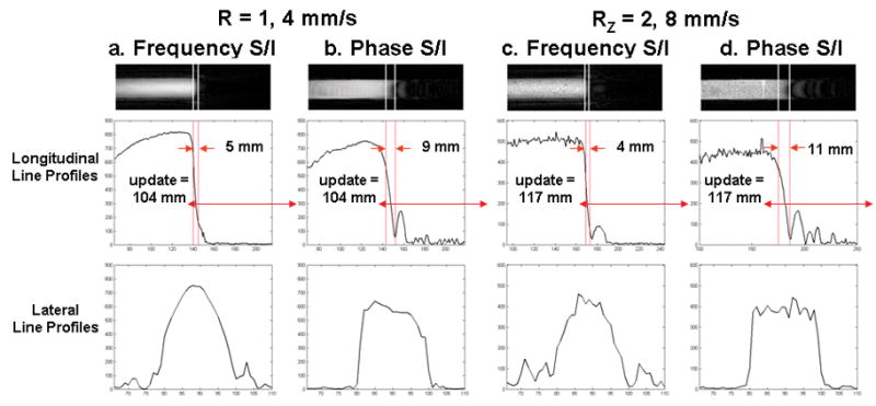
Comparison of leading edge artifact for motion along the frequency (a,c) vs. phase (b,d) encoding directions with an EC CAPR acquisition for the cases of no SENSE acceleration (R = 1) at a bolus velocity of 4 mm/s (a,b) and R_Z = 2 at a bolus velocity of 8 mm/s (c,d). A selected time frame and the corresponding longitudinal and lateral line profiles are shown.

Fig. 8 shows selected frames from EC CAPR acquisitions with 2D SENSE acceleration factors 1, 2, 4, and 7.3, all acquired at a bolus velocity of 8 mm/s. Again, the sampling pattern over time is shown on the images. The orange block does not change width with increased R, as the k-space center is fixed at 400 points for all accelerations. The other colored blocks represent the subsequent high pass vanes sampled referenced to Fig. 2a-b. For these images a Delay 3 reconstruction was used to show the effects of temporal footprint on anticipation artifact. With increasing SENSE acceleration, the length of the anticipation artifact (arrows, a and b) is reduced and the sharpness of the leading edge is improved.

Figure 8.

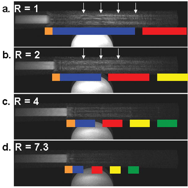
Selected frames from an EC CAPR acquisitions (bolus velocity 8 mm/s) with varying 2D SENSE accelerations: (a) R=1, (b) R=2, (c) R=4, (d) R=7.3 reconstructed with Delay 3. The k-space sampling pattern is superimposed in color. Motion is left to right. With increased SENSE acceleration there is a decrease in the temporal footprint, decreased anticipation artifact (arrows, a and b), and improved leading edge sharpness.

Fig. 9 shows images and longitudinal line profiles comparing the random and standard EC ordered CAPR sampling at a bolus speed of 4 mm/s with R =1 and R = 7.3. Vertical lines on the images and line profiles mark the 75% and 25% maximum signal positions used to determine the extent of leading edge blur. The measured blur width and the distance traveled by the bolus phantom over one image update are shown on the line profiles.

Figure 9.

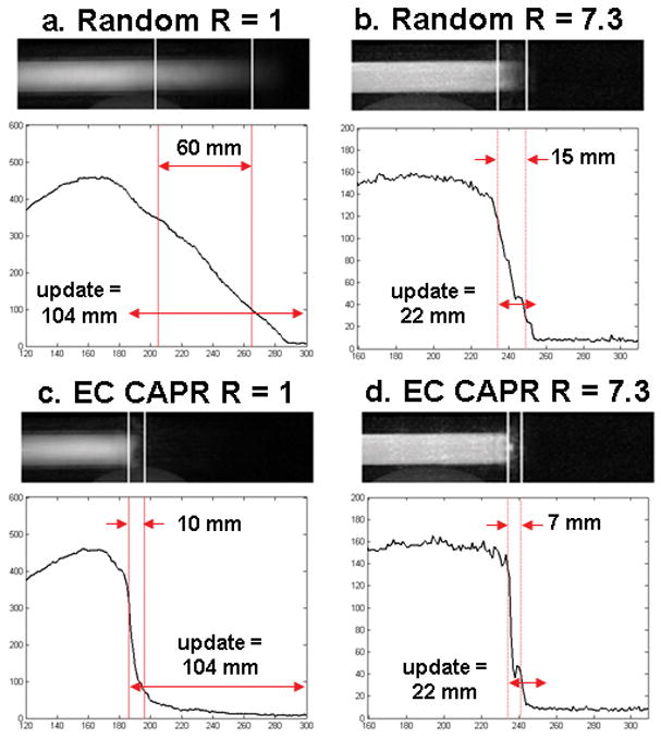
Single frame from motion studies (bolus velocity 4 mm/s) using random, (a) R=1 and (b) R=7.3, and standard EC CAPR, (c) R=1 and (d) R=7.3, sampling. Shown with each image is the corresponding longitudinal line profile. Vertical lines mark the 75% and 25% signal positions used to quantify the width of the lead edge blur. Double arrows indicate the blur width and the distance traveled by the phantom each time frame.

Fig. 10 shows images of the leading edge of the bolus vial and longitudinal line profiles for EC CAPR Delay 0 with only one central k-space sampling (a) and with the averaging of two (b), three (c), and four (d) central k-space samplings where for the latter three cases k-space center samplings just prior to that used in (a) were progressively averaged.

Figure 10.

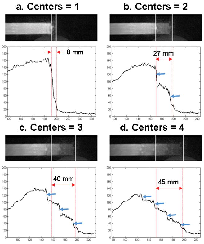
A selected frame and longitudinal line profiles are shown for an EC CAPR acquisition (R = 7.3, bolus velocity 4 mm/s) that was reconstructed by averaging one (a), two (b), three (c), or four (d) k-space centers. When multiple centers are averaged there is a decrease in signal and increase in blurring of the leading edge and the appearance of multiple edges (blue arrows) in accordance with the number of centers averaged.

Fig. 11 shows images of the leading and trailing edges of the bolus vial for an EC CAPR acquisition reconstructed with Delay 3 and Delay 0. The sampling pattern over k-space and time is shown on the images to illustrate the ordering of peripheral k-space with respect to the center (orange sections) for the reconstruction. With Delay 3 reconstruction, there is extensive anticipation artifact (arrows, a). With a Delay 0 reconstruction, there is diminished anticipation artifact but an analogous persistence artifact at the trailing edge (arrows, d).

Figure 11.

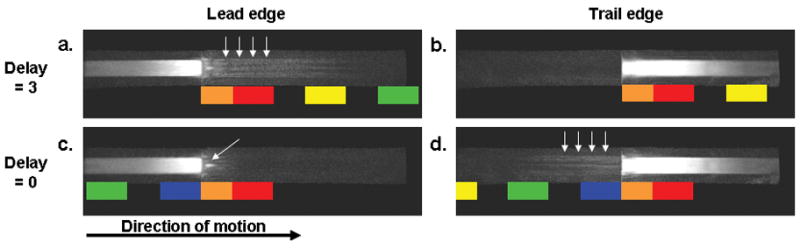
Selected frames are shown using Delay 3 and Delay 0 reconstructions for an EC CAPR acquisition, SENSE (R=7.3), with a bolus velocity of 16 mm/s. The leading and trailing edges are shown for Delay 3 (a,b) and Delay 0 (c,d). With Delay 3 there is an extended anticipation artifact and Delay 0 an extended persistence artifact. The arrows in a and d highlight these anticipation and persistence artifacts respectively. The arrow in c highlights a specific artifact discussed in the text.

Fig. 12 shows results from an in vivo study acquired using EC CAPR with 2D SENSE (R = 8) and reconstructed with Delay 0 (a1–a3), Delay 3 (b1–b3), Delay 0 averaging four centers (c1–c3), and Delay −1 (d1–d3). The MIP images are shown with dark vessels per our clinical practice. For each reconstruction a selected time frame is shown at which arterial signal is first apparent at the level of the left mid-calf. For Delay 0 (a) and Delay −1 (d) the same k-space center is used to reconstruct this frame. For the Delay 3 reconstruction (b) the same peripheral k-space sections are used as for Delay 0, but the center is different according to Fig. 3. For (c) the signals from four consecutively measured centers were averaged as shown schematically; the peripheral k-space sections matched those of (a) and (b).

Figure 12.

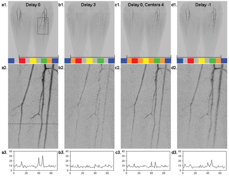
A selected time frame from an in vivo study using an EC CAPR (R = 8) acquisition with data selected four different ways: (a1–a3) Delay 0 reconstruction; (b1–b3) Delay 3 reconstruction; (c1–c3) Delay 0 reconstruction but with averaging of four consecutive central samplings; (d1–d3) Delay −1 reconstruction. Parts (a1–d1) show the coronal MIP of the full 40 cm S/I FOV. Superimposed in colored blocks for each is the sampling pattern of k-space, and shown within the black bracket is the set of k-space samples used for actual reconstruction. The duration of one update, consisting of one orange and one adjacent block, is 4.9 s. Parts (a2–d2) are enlargements of the region identified in the dashed box of (a1) and were generated by 4.65× zero padding of k-space. Parts (a3–d3) are signal profiles across a line in the corresponding enlarged image, where the line is identified in (a2). The Delay 0 reconstruction with no averaging (a1–a2–a3) is the preferred method.

DISCUSSION

We have shown how a computer-controlled phantom, which simulates an advancing contrast bolus, can be used to assess the performance of various acquisition techniques in time-resolved 3D contrast-enhanced MRA. Specifically, we have studied centricity and consistency of view sampling and the effects of data selection for reconstruction and of 2D parallel acquisition.

The comparison of different view orders in Figs. 4 and 5 showed that orders that are centric in both k_Y and k_Z provided both improved positional accuracy and improved leading edge sharpness. Quantitative results are tabulated in Tables 1 and 2. Advantages of centric sampling such as robustness to motion artifact and high intrinsic venous suppression have been previously described (9), and this work has taken the analysis of the effects of view ordering to a higher level of detail and precision.

Comparing results for each view order from Case I to Case II in Table 2, we would expect the blur width to increase with increased bolus velocity and decrease with more rapid sampling provided by SENSE. However, these changes in velocity and SENSE acceleration do not affect all view orders in the same manner. For both cases REC CAPR shows minimal leading edge blur because the lowest spatial frequency views are acquired last in the time series. For EC CAPR and Centric k_Y-k_Z because the central region is kept fixed at 400 points for both accelerations, the effect of increased velocity dominates over that of SENSE acceleration and the blur increases somewhat. The greatly decreased blur in the Centric k_Y images from Case I to II is due to the dependence of the blur width on image update time for this view order, as data from the center of k_Z is acquired throughout the update interval.

Another aspect of view ordering studied in Figs. 4 and 5 is the direction of centric sampling. The EC versus REC CAPR acquisitions demonstrated tradeoffs between longitudinal and lateral resolution. In the EC acquisition there was leading edge artifact due to the continued forward progress of the bolus while the final vane set of high spatial frequency data was acquired. The REC acquisition provided for a very sharp leading edge in the longitudinal direction, but due to the lack of high spatial frequency data at the furthest bolus extent, the lead edge in the lateral direction was noisier and broadened laterally compared to the EC acquisition, and for these reasons REC was not further considered.

In this work consistency of sampling of specific view orders was studied by determining the accuracy in portrayal of linear motion over a set of equal update time intervals. CAPR, Centric k_Y-k_Z and Centric k_Y all showed equal spacing of the bolus leading edge between image updates (e.g. Fig. 4, CAPR and Centric k_Y), with R²≈1.00 when position was plotted versus time over consecutive frames (Fig. 6). Accuracy in portraying the absolute velocity of continuous linear motion is provided by consistency in k-space sampling from frame to frame.

Phantom studies were generally performed with frequency encoding along the direction of motion. However, in most CE-MRA applications, there are vessels in which blood flow is along a phase encoding direction. When phase encoding was performed along the direction of motion in our phantom experiments (Fig. 7b,d) the longitudinal resolution was somewhat degraded, showing extended leading edge blur and oscillatory signal artifact, but the lateral resolution was improved relative to frequency encoding S/I.

Not surprisingly, implementing 2D SENSE allowed for improved freezing of bolus motion. The decreased image update time and temporal footprint provided decreased length of anticipation artifact and improved edge sharpness (Fig. 8). Improved temporal resolution, while maintaining k-space coverage and spatial resolution, proves particularly beneficial at high bolus velocities where acquiring multiple updates over one FOV would not be possible otherwise.

Comparing the random and EC CAPR acquisitions (Fig. 9) without and with SENSE acceleration allowed for evaluation of the relative effect of view ordering and parallel imaging. The randomly ordered acquisition (a) showed marked blurring of the bolus leading edge (blur length = 60 mm) reflecting sampling of some central k-space views over an extended distance during an image update time. Incorporation of 2D SENSE (R = 7.3) to the random acquisition (b) provided a sharper leading edge (blur length = 15 mm) due to the decrease in image update time, but the leading edge is still not as sharp as for the EC acquisition even without SENSE (c). This study demonstrates the value for freezing motion of acquiring the central k-space points quickly and contiguously. Sampling patterns such as the random pattern studied here or radial acquisition (35,36) have an inherent temporal unsharpness because the k-space center is sampled over an extended duration.

The superior performance of centric versus random ordering evident in Fig. 9 may seem to contradict that observed in e.g. Ref. (31). The reason for this discrepancy is, we believe, due to the intrinsic assumption in this work that the desired frame rate of the reconstructed image series is known a priori, and that the view order is selected to match this frame rate prior to data acquisition. That is to say, if additional images reconstructed at intermediate time points are desired once data acquisition has been completed, such images would lose some degree of fidelity compared to those formed at the predefined time points. With randomized view orders, images can be reconstructed at arbitrary time points after data acquisition, and all images might be expected to have equivalent quality. We do not believe that the requirement for a predefined frame rate is a limitation, as this is typically known for a given application. The CAPR sequence can be adapted to multiple combinations of frame rate, FOV, and spatial resolution different from those here, such as CE-MRA of the intracranial vasculature (23).

Fig. 10 shows that the averaging of multiple samplings of the k-space center in effect causes superposition of multiple leading edges (blue arrows). Methods which use temporal interpolation of two central k-space samplings to estimate the object status at some intermediate time e.g. that of Ref (13) are prone to similar artifact. When averaging is performed there is a significant reduction in signal and increase in longitudinal blur at the bolus leading edge. This is an example of the comment in the preceding paragraph. An image formed at an intermediate time using interpolation suffers some loss of temporal fidelity. Interpolation disrupts the consistency with which k-space is sampled for the non-interpolated frames.

Another question studied is how the views should be assigned for reconstruction. There is a choice in regards to the location of the sampling of the k-space center within the temporal footprint. With a Delay 3 reconstruction there is a pronounced anticipation artifact (Fig. 11a) due to the acquisition of the high spatial frequency data throughout an extended time period over which the bolus continues to advance. In Delay 0 reconstruction there is an extended persistence artifact (Fig. 11d) from using high spatial frequency data predominantly acquired before central k-space is sampled. Since a primary interest of time-resolved CE-MRA is accurate depiction of the leading edge of a contrast bolus moving through the vessels, the Delay 0 reconstruction with an EC acquisition is thus appropriate. Delay 0 reconstruction preserves many of the benefits of standard EC acquisition (9) in that one vane set of high spatial frequencies is sampled after the central views thus allowing high lateral resolution. At the same time, the anticipation artifact is kept relatively limited, an artifact which mimics signals from later-filling structures such as veins.

As illustrated in the in vivo CE-MRA study in Fig. 12, the Delay 0 (a1–a3) sort shows the highest signal and sharpest spatial resolution. Delay 3 reconstruction (b1–b3) shows discontinuously appearing vessels, as the signal in this frame is due solely to the acquisition of high spatial frequencies with the continued advancement of the contrast bolus beyond the sampling of the k-space center. This is analogous to the anticipation artifact of Figs. 8 and 11a. With averaging of multiple k-space centers (c1–c3) there is decreased SNR because all but the last sampling of the k-space center were done prior to contrast material arrival at the location of the bolus leading edge for the reconstructed time frame. In the Delay −1 reconstruction (d1–d3) there is lateral degradation of spatial resolution at the contrast bolus leading edge, as seen in the widened peaks of the plot of Fig. d3. This is due to the inclusion of high spatial frequency data largely acquired prior to contrast material arrival at the location of the depicted bolus leading edge and thus having negligible signal.

In some highly accelerated acquisitions done with the EC CAPR or Centric k_Y-k_Z view order, a small region of intense signal appeared along the central axis of the bolus leading edge (e.g. Fig. 11c, arrow). This lead edge ‘signal bead’ was investigated in more detail. Numerical simulations confirm that the signal bead arises from not sampling the centermost of k-space at the furthest extent of bolus travel for a given reconstruction. The signal bead artifact has not been visible in in vivo studies probably because contrast arrival is not as abrupt as that here.

A potential limitation of this study is the sharp leading edge of the simulated bolus. Although this may mimic contrast bolus arrival which is more sudden than that encountered physiologically, the use of a stringent test to assess performance can still be worthwhile. In vivo, the leading edge of the contrast bolus can often be well demarcated, and its appearance dependent on the acquisition technique, as illustrated in Fig. 12. We have seen similar behavior in dozens of other CE-MRA studies in vivo. Although it was beyond the scope of this work to study in detail other methods for time-resolved CE-MRA such as TRICKS (13), keyhole (16,22), TWIST (37) and HYPR (25), we believe that a number of the findings of this work, as well as the criteria for evaluation of performance, are general and potentially applicable to these other methods.

CONCLUSIONS

Phantom studies have confirmed our hypotheses that compact sampling of the k-space center using view orders centric in both k_Y and k_Z provides a sharp and accurate bolus leading edge, effectively freezing motion at a given reconstruction time frame. At physiological velocities encountered in the lower legs, blur of the leading edge is typically well under 20% of the distance traveled per image update. Consistency of k-space sampling from frame to frame provides accurate portrayal of linear motion. Sharpness is degraded by temporal averaging and interpolation. Reconstructing time-resolved data sets using predominantly high pass data acquired before the k-space center for an update allows for decreased anticipation artifact. These findings are borne out in vivo.

References

- 1.Prince MR, Grist TM, Debatin JF, editors. 3D Contrast MR Angiography. 3. Berlin: Springer; 2003. [Google Scholar]
- 2.Schneider G, Prince MR, Meaney JFM, Ho VB, editors. Magnetic resonance angiography: techniques, indications and practical applications. Milan: Springer; 2005. [Google Scholar]
- 3.Zhang H, Maki JH, Prince MR. 3D contrast-enhanced MR angiography. J Magn Reson Imaging. 2007;25:13–25. doi: 10.1002/jmri.20767. [DOI] [PubMed] [Google Scholar]
- 4.Maki JH, Prince MR, Londy FJ, Chenevert TL. The effects of time varying intravascular signal intensity and k-space acquisition order on three-dimensional MR angiography image quality. J Magn Reson Imaging. 1996;6:642–651. doi: 10.1002/jmri.1880060413. [DOI] [PubMed] [Google Scholar]
- 5.Svensson J, Petersson JS, Stahlberg F, Larsson EM, Leander P, Olsson LE. Image artifacts due to a time-varying contrast medium concentration in 3D contrast-enhanced MRA. J Magn Reson Imaging. 1999;10:919–928. doi: 10.1002/(sici)1522-2586(199912)10:6<919::aid-jmri3>3.0.co;2-w. [DOI] [PubMed] [Google Scholar]
- 6.Earls JP, Rofsky NM, DeCorato DR, Krinsky GA, Weinreb JC. Hepatic arterial-phase dynamic gadolinium-enhanced MR imaging: optimization with a test examination and a power injector. Radiology. 1997;202:268–273. doi: 10.1148/radiology.202.1.8988222. [DOI] [PubMed] [Google Scholar]
- 7.Foo TK, Saranathan M, Prince MR, Chenevert TL. Automated detection of bolus arrival and initiation of data acquisition in fast, three-dimensional, gadolinium-enhanced MR angiography. Radiology. 1997;203:275–280. doi: 10.1148/radiology.203.1.9122407. [DOI] [PubMed] [Google Scholar]
- 8.Wilman AH, Riederer SJ, King BF, Debbins JP, Rossman PJ, Ehman RL. Fluoroscopically triggered contrast-enhanced three-dimensional MR angiography with elliptical centric view order: application to the renal arteries. Radiology. 1997;205:137–146. doi: 10.1148/radiology.205.1.9314975. [DOI] [PubMed] [Google Scholar]
- 9.Wilman AH, Riederer SJ. Performance of an elliptical centric view order for signal enhancement and motion artifact suppression in breath-hold three-dimensional gradient echo imaging. Magn Reson Med. 1997;38:793–802. doi: 10.1002/mrm.1910380516. [DOI] [PubMed] [Google Scholar]
- 10.Willinek WA, Gieseke J, Conrad R, Strunk H, Hoogeveen R, von Falkenhausen M, Keller E, Urbach H, Kuhl CK, Schild HH. Randomly segmented central k-space ordering in high-spatial-resolution contrast-enhanced MR angiography of the supraaortic arteries: initial experience. Radiology. 2002;225:583–588. doi: 10.1148/radiol.2252011167. [DOI] [PubMed] [Google Scholar]
- 11.Wang Y, Lee HM, Khilnani NM, Trost DW, Jagust MB, Winchester PA, Bush HL, Sos TA, Sostman HD. Bolus-chase MR digital subtraction angiography in the lower extremity. Radiology. 1998;207:263–269. doi: 10.1148/radiology.207.1.9530326. [DOI] [PubMed] [Google Scholar]
- 12.Hennig J, Scheffler K, Laubenberger J, Strecker R. Time-resolved projection angiography after bolus injection of contrast agent. Magn Reson Med. 1997;37:341–345. doi: 10.1002/mrm.1910370306. [DOI] [PubMed] [Google Scholar]
- 13.Korosec FR, Frayne R, Grist TM, Mistretta CA. Time-resolved contrast-enhanced 3D MR angiography. Magn Reson Med. 1996;36:345–351. doi: 10.1002/mrm.1910360304. [DOI] [PubMed] [Google Scholar]
- 14.Mistretta CA, Grist TM, Korosec FR, Frayne R, Peters DC, Mazaheri Y, Carroll TJ. 3D time-resolved contrast-enhanced MR DSA: advantages and tradeoffs. Magn Reson Med. 1998;40:571–581. doi: 10.1002/mrm.1910400410. [DOI] [PubMed] [Google Scholar]
- 15.Riederer SJ, Tasciyan T, Farzaneh F, Lee JN, Wright RC, Herfkens RJ. MR fluoroscopy: technical feasibility. Magn Reson Med. 1988;8:1–15. doi: 10.1002/mrm.1910080102. [DOI] [PubMed] [Google Scholar]
- 16.van Vaals JJ, Brummer ME, Dixon WT, Tuithof HH, Engels H, Nelson RC, Gerety BM, Chezmar JL, den Boer JA. “Keyhole” method for accelerating imaging of contrast agent uptake. J Magn Reson Imaging. 1993;3:671–675. doi: 10.1002/jmri.1880030419. [DOI] [PubMed] [Google Scholar]
- 17.Pruessmann KP, Weiger M, Scheidegger MB, Boesiger P. SENSE: sensitivity encoding for fast MRI. Magn Reson Med. 1999;42:952–962. [PubMed] [Google Scholar]
- 18.Sodickson DK, Manning WJ. Simultaneous acquisition of spatial harmonics (SMASH): fast imaging with radiofrequency coil arrays. Magn Reson Med. 1997;38:591–603. doi: 10.1002/mrm.1910380414. [DOI] [PubMed] [Google Scholar]
- 19.Griswold MA, Jakob PM, Heidemann RM, Nittka M, Jellus V, Wang J, Kiefer B, Haase A. Generalized autocalibrating partially parallel acquisitions (GRAPPA) Magn Reson Med. 2002;47:1202–1210. doi: 10.1002/mrm.10171. [DOI] [PubMed] [Google Scholar]
- 20.Weiger M, Pruessmann KP, Boesiger P. 2D SENSE for faster 3D MRI. Magma. 2002;14:10–19. doi: 10.1007/BF02668182. [DOI] [PubMed] [Google Scholar]
- 21.Hu HH, Madhuranthakam AJ, Kruger DG, Glockner JF, Riederer SJ. Combination of 2D sensitivity encoding and 2D partial Fourier techniques for improved acceleration in 3D contrast-enhanced MR angiography. Magn Reson Med. 2006;55:16–22. doi: 10.1002/mrm.20742. [DOI] [PMC free article] [PubMed] [Google Scholar]
- 22.Willinek WA, Hadizadeh DR, von Falkenhausen M, Urbach H, Hoogeveen R, Schild HH, Gieseke J. 4D time-resolved MR angiography with keyhole (4D-TRAK): more than 60 times accelerated MRA using combination of CENTRA, keyhole, and SENSE at 3.0T. J Magn Reson Imaging. 2008;27:1455–1460. doi: 10.1002/jmri.21354. [DOI] [PubMed] [Google Scholar]
- 23.Haider CR, Hu HH, Campeau NG, Huston J, 3rd, Riederer SJ. 3D high temporal and spatial resolution contrast-enhanced MR angiography of the whole brain. Magn Reson Med. 2008;60:749–760. doi: 10.1002/mrm.21675. [DOI] [PMC free article] [PubMed] [Google Scholar]
- 24.Taschner CA, Gieseke J, Le Thuc V, Rachdi H, Reyns N, Gauvrit JY, Leclerc X. Intracranial arteriovenous malformation: time-resolved contrast-enhanced MR angiography with combination of parallel imaging, keyhole acquisition, and k-space sampling techniques at 1.5 T. Radiology. 2008;246:871–879. doi: 10.1148/radiol.2463070293. [DOI] [PubMed] [Google Scholar]
- 25.Mistretta CA, Wieben O, Velikina J, Block W, Perry J, Wu Y, Johnson K. Highly constrained backprojection for time-resolved MRI. Magn Reson Med. 2006;55:30–40. doi: 10.1002/mrm.20772. [DOI] [PMC free article] [PubMed] [Google Scholar]
- 26.Doyle M, Walsh EG, Blackwel lGG, Pohost GM. Block regional interpolation scheme for k-space (BRISK): a rapid cardiac imaging technique. Magn Reson Med. 1995;33:163–170. doi: 10.1002/mrm.1910330204. [DOI] [PubMed] [Google Scholar]
- 27.Huang Y, Wright GA. Time-resolved MR angiography with limited projections. Magn Reson Med. 2007;58:316–325. doi: 10.1002/mrm.21312. [DOI] [PubMed] [Google Scholar]
- 28.Carroll TJ, Korosec FR, Swan JS, Hany TF, Grist TM, Mistretta CA. The effect of injection rate on time-resolved contrast-enhanced peripheral MRA. J Magn Reson Imaging. 2001;14:401–410. doi: 10.1002/jmri.1200. [DOI] [PubMed] [Google Scholar]
- 29.Keith L, Kecskemeti S, Velikina J, Mistretta CA. Simulation of relative temporal resolution of time-resolved MRA sequences. Magn Reson Imaging. 2008;60:398–404. doi: 10.1002/mrm.21658. [DOI] [PMC free article] [PubMed] [Google Scholar]
- 30.Madhuranthakam AJ, Hu HH, Barger AV, Haider CR, Kruger DG, Glockner JF, Huston J, 3rd, Riederer SJ. Undersampled elliptical centric view-order for improved spatial resolution in contrast-enhanced MR angiography. Magn Reson Med. 2006;55:50–58. doi: 10.1002/mrm.20726. [DOI] [PubMed] [Google Scholar]
- 31.Parrish T, Hu X. Continuous update with random encoding (CURE): a new strategy for dynamic imaging. Magn Reson Med. 1995;33:26–36. doi: 10.1002/mrm.1910330307. [DOI] [PubMed] [Google Scholar]
- 32.Haider CR, Campeau N, Glockner JF, Huston J, Riederer SJ. Highly accelerated (>10x) parallel acquisition for 3D time-resolved CE-MRA of the calves. Proc Joint Ann Mtg ISMRM-ESMRMB. 2008:19. [Google Scholar]
- 33.Johnson CP, Haider CR, Rossman PJ, Hulshizer TC, Borisch EA, Riederer SJ. Coil design for highly accelerated 2D SENSE MRA of the lower legs. Proc Joint Ann Mtg ISMRM-ESMRMB. 2008 [Google Scholar]
- 34.Madhuranthakam AJ, Kruger DG, Riederer SJ, Glockner JF, Hu HH. Time-resolved 3D contrast-enhanced MRA of an extended FOV using continuous table motion. Magn Reson Med. 2004;51:568–576. doi: 10.1002/mrm.10729. [DOI] [PubMed] [Google Scholar]
- 35.Peters DC, Korosec FR, Grist TM, Block WF, Holden JE, Vigen KK, Mistretta CA. Undersampled projection reconstruction applied to MR angiography. Magn Reson Med. 2000;43:91–101. doi: 10.1002/(sici)1522-2594(200001)43:1<91::aid-mrm11>3.0.co;2-4. [DOI] [PubMed] [Google Scholar]
- 36.Du J, Carroll TJ, Wagner HJ, Vigen K, Fain SB, Block WF, Korosec FR, Grist TM, Mistretta CA. Time-resolved, undersampled projection reconstruction imaging for high-resolution CE-MRA of the distal runoff vessels. Magn Reson Med. 2002;48:516–522. doi: 10.1002/mrm.10243. [DOI] [PubMed] [Google Scholar]
- 37.Lim RP, Shapiro M, Wang EY, Law M, Babb JS, Rueff LE, Jacob JS, Kim S, Carson RH, Mulholland TP, Laub G, Hecht EM. 3D time-resolved MR angiography (MRA) of the carotid arteries with time-resolved imaging with stochastic trajectories: comparison with 3D contrast-enhanced bolus-chase MRA and 3D time-of-flight MRA. Am J Neuroradiol. 2008;29:1847–1854. doi: 10.3174/ajnr.A1252. [DOI] [PMC free article] [PubMed] [Google Scholar]