Comparison of apparent diffusion coefficients (ADC) and distributed diffusion coefficients (DDC) in high-grade gliomas

Abstract

Purpose

To compare apparent diffusion coefficients (ADCs) with distributed diffusion coefficients (DDCs) in high-grade gliomas.

Materials and Methods

Twenty patients with high-grade gliomas prospectively underwent diffusion-weighted magnetic resonance imaging. Traditional ADC maps were created using b-values of 0 and 1000 s/mm². In addition, DDC maps were created by applying the stretched-exponential model using b-values of 0, 1000, 2000, and 4000 s/mm². Whole-tumor ADCs and DDCs (in 10^-3 mm²/s) were measured and analyzed with a paired t test, Pearson's correlation coefficient, and the Bland-Altman method.

Results

Tumor ADCs (1.14 ± 0.26) were significantly lower (P = 0.0001) than DDCs (1.64 ± 0.71). Tumor ADCs and DDCs were strongly correlated (R = 0.9716; P < 0.0001), but mean bias ± limits of agreement between tumor ADCs and DDCs was -0.50 ± 0.90. There was a clear trend toward greater discordance between ADC and DDC at high ADC values.

Conclusion

Under the assumption that the stretched-exponential model provides a more accurate estimate of the average diffusion rate than the mono-exponential model, our results suggest that for a little diffusion attenuation the mono-exponential fit works rather well for quantifying diffusion in high-grade gliomas, whereas it works less well for a greater degree of diffusion attenuation.

Introduction

Magnetic resonance (MR) imaging plays an important role in the detection and evaluation of brain tumors. In addition to conventional MR imaging, diffusion-weighted MR imaging (DWI) is developing as an important method for the assessment of brain tumors (1). DWI allows visualization and quantification of the random (Brownian) of water molecules driven by thermal energy (1-3). Because the presence of impediments such as cell membranes, organelles and macromolecules that interfere with the free movement of water molecules, diffusion in biological tissue is quantified by means of an apparent diffusion coefficient (ADC) (1-3). Measurement of ADC would be expected to be useful in brain tumor assessment because variations in water mobility can be found within tumors for various reasons (e.g. necrosis, variations in cellularity) and adjacent to tumors (e.g. vasogenic edema), this likely provides information not readily available from conventional MR imaging (1).

The ADC is most frequently calculated using an implicit mono-exponential model, as follows:

$$S\mathit{(}b\mathit{)}/S_{\mathit{0}}=\mathit{\text{exp}}\mathit{(}-b\times \mathit{\text{ADC}}\mathit{)},$$ [1]

where S(b) is the signal magnitude with diffusion weighting b, S₀ is the signal magnitude with no diffusion weighting, and b is the b-value, which is calculated for a standard square-shaped gradient pulse pair as follows:

$$b={\gamma }^{\mathit{2}}\times G^{\mathit{2}}\times {\delta }^{\mathit{2}}\mathit{(}\Delta -\delta /\mathit{3}\mathit{)}.$$ [2]

Here, γ is the gyromagnetic ratio (42.58 MHz/T for hydrogen), G is the strength of the motion probing gradients (MPGs), δ is the duration of one MPG pulse, and Δ is the interval between the leading edges of the MPG pulses (1-3). However, diffusion-weighted signal decay in the brain and in brain tumors has been shown to be multi-exponential (4) particularly when a wide range of b-values are acquired (eg. b ≥ 3000 s/mm²). An obvious extension beyond mono-exponential behaviour is the bi-exponential model which may be a better way to describe the admixture of multiple exponential signal decays (4). The bi-exponentional model allows for a fast diffusing proton pool (originally assumed to correspond to extracellular diffusion) and a slow diffusing proton pool (originally assumed to correspond to intracellular diffusion) coexisting inside each voxel, and is described as follows (4):

$$S\mathit{(}b\mathit{)}/S_{\mathit{0}}=V_{\mathit{1}}\times \mathit{\text{exp}}\mathit{(}-b\times D_{\mathit{1}}\mathit{)}+V_{\mathit{2}}\times \mathit{\text{exp}}\mathit{(}-b\times D_{\mathit{2}}\mathit{)},$$ [3]

where V₁ and V₂ are the volume fractions of the fast and slowly diffusing pools (V₁ + V₂ = 1), and D₁ and D₂ are the corresponding ADCs. However, the bi-exponential model is also an oversimplification of tissue water movement in reality, and it is probably more realistic to assume a larger number (>2) of intravoxel proton pools with a continous distribution of diffusion coefficients (5). Moreover, detailed studies of animal and human brain tissue have determined that assumptions of fast and slow compartments being extra- and intracellular water pools, respectively, are not supported by empirical data (6). To overcome the difficulty of making assumptions about the number of intravoxel proton pools with different diffusion coefficients in biological tissue, Bennett et al. (5, 7, 8) introduced the stretched-exponential model. The stretched-exponential model is mathematically described as follows:

$$S\mathit{(}b\mathit{)}/S_{\mathit{0}}=\mathit{\text{exp}}\mathit{(}-{\mathit{(}b\times \mathit{\text{DDC}}\mathit{)}}^{\alpha }\mathit{)},$$ [4]

where the index α relates to intravoxel water diffusion heterogeneity, varying between 0 and 1, and the DDC is the distributed diffusion coefficient, representing mean intravoxel diffusion rates. Interestingly, this model introduces a new parameter (α), which provides a new type of image contrast (different from conventional DWI), that relates to the degree of intravoxel water diffusion heterogeneity. By inspection of equation (1), it should be clear an α = 1 is equivalent to mono-exponential diffusion-weighted signal decay, thus low intravoxel diffusion heterogeneity. Conversely an α near 0 indicates a higher degree of multi-exponential signal decay (5, 7, 8); this convention maintains consistency with Bennett et al.'s (5, 7, 8) definition of α as a heterogeneity index. Another key point worth emphasis is that the term “heterogeneity” in this context refers to intravoxel heterogeneity of exponential decay, as opposed to intervoxel heterogeneity of diffusion coefficients as often is the case. The DDC has the properties and units of a standard diffusion coefficient and can be thought of as the composite of individual ADCs weighted by the volume fraction of water in each part of the continuous distribution of ADCs. Given the fact tissue exhibits non-mono-exponential behavior, the stretched-exponential model at a minimum provides a more complete and accurate empiric description of tissue water diffusion since the model is able to fit a variety of observed decay shapes using only two fit parameters (5, 7, 8). Nevertheless, the conventional mono-exponential ADC (simply referred to as “ADC” in the remainder of this manuscript), usually calculated by obtaining one image without diffusion-weighting (i.e. b = 0 s/mm²) and one image with relatively high diffusion-weighting (in the brain usually b = 1000 s/mm²), is still the most prevalent method for quantifying diffusion in clinical practice (9, 10). However, especially in highly heterogeneous tissue, such as high-grade gliomas, the ADC may be nonideal for use, because it is only an approximation of the distribution of diffusion rates in a voxel (5, 7, 8). The aim of this study was therefore to compare ADC to DDC in high-grade gliomas.

Materials and Methods

Patients

This study was approved by the local institutional review board and written informed consent was obtained from all participants. Twenty patients with high-grade glioma (WHO grade III: N=3, WHO grade IV: N=17, 10 men, 10 women, mean age 58.2 years [range, 20-89 years]) prospectively underwent DWI of the brain, before any treatment was started. Exclusion criteria were general contraindications to MR imaging, such as implanted pacemaker and claustrophobia. Patient characteristics are displayed in Table 1.

Table 1.

Patient characteristics.

Case	Age	Sex	WHO grade	Location	ADC (×10-3 mm2/s)*	DDC (×10-3 mm2/s)*	α*
1	28	M	III	Frontal/temporal	0.97 ± 0.19	1.01 ± 0.37	0.55 ± 0.05
2	29	M	III	Frontal	1.47 ± 0.45	2.80 ± 1.65	0.41 ± 0.14
3	75	F	IV	Temporal	1.03 ± 0.27	1.18 ± 0.59	0.63 ± 0.11
4	75	F	IV	Temporal	1.09 ± 0.38	1.41 ± 1.00	0.64 ± 0.11
5	20	M	IV	Frontal	1.41 ± 0.44	2.31 ± 1.43	0.53 ± 0.13
6	73	M	IV	Frontal	1.52 ± 0.66	2.64 ± 1.77	0.53 ± 0.17
7	56	M	IV	Temporal/frontal	1.04 ± 0.18	1.13 ± 0.46	0.68 ± 0.06
8	40	F	IV	Occipital/temporal	1.01 ± 0.55	1.26 ± 1.26	0.59 ± 0.14
9	69	M	IV	Temporal	1.40 ± 0.59	2.41 ± 1.63	0.52 ± 0.12
10	78	F	IV	Temporal	1.18 ± 0.55	1.92 ± 1.65	0.55 ± 0.17
11	61	M	IV	Parietal/occipital	0.75 ± 0.15	0.68 ± 0.32	0.65 ± 0.10
12	51	F	IV	Occipital/parietal	0.70 ± 0.35	0.77 ± 0.88	0.70 ± 0.16
13	61	F	IV	Temporal	1.37 ± 0.40	2.28 ± 1.40	0.53 ± 0.13
14	68	M	IV	Parietal	1.20 ± 0.26	1.54 ± 0.79	0.58 ± 0.08
15	89	F	IV	Temporal/occipital	1.42 ± 0.35	2.58 ± 1.43	0.45 ± 0.10
16	46	M	IV	Temporal/frontal	1.46 ± 0.40	2.43 ± 1.28	0.53 ± 0.10
17	63	F	III	Temporal	0.76 ± 0.15	0.73 ± 0.18	0.75 ± 0.09
18	65	F	IV	Temporal	1.07 ± 0.21	1.21 ± 0.53	0.61 ± 0.08
19	62	M	IV	Temporal	0.95 ± 0.26	1.09 ± 0.76	0.56 ± 0.15
20	55	F	IV	Occipital	1.08 ± 0.45	1.48 ± 1.29	0.59 ± 0.12

Notes:

^*Mean, whole-tumor values

Phantom

To support the experimental findings in the patients, a water phantom with varying local temperatures was created and scanned with the same parameters for DWI as were used in the patients. The variable temperature phantom provides a range of diffusion values, although since the material was simple water the signal decay should appear as mono-exponential (i.e. α≈1).

MR imaging

All patients and the phantom were examined with a 3.0 T MR scanner (Achieva 3.0 T Quasar Dual, Philips Healthcare, Best, The Netherlands) using an eight-channel head coil. DWI was performed using a single-shot spin-echo (SE) echo-planar imaging (EPI) sequence, with the following parameters: repetition time/echo time of 8700/60 ms, image acquisiton in the axial plane, slice thickness/gap of 4/1 mm, number of slices of 28, field of view of 240 × 240 mm, acquisition matrix of 128 × 99, motion probing gradients (MPGs) in three orthogonal axes, b values of 0, 1000, 2000, and 4000 s/mm², number of signal averages of 1 (for b-value of 0 s/mm²), 2 (for b-value of 1000 s/mm²), and 3 (for b-values of 2000 and 4000 s/mm²) (in order to increase signal at higher b-values), half scan factor of 0.733, parallel imaging (SENSitivity Encoding [SENSE]) factor of 3, EPI factor of 35, spectral presaturation inversion recovery (SPIR) fat suppression, acquired voxel size of 1.88 × 2.41 × 4.00 mm³, reconstructed voxel size of 0.94 × 0.94 × 4.00 mm³, and total scan time of 4 minutes and 30 s. In all patients, routine anatomical pre- and post- post-gadolinium 3D T1-weighted fast field echo, turbo SE axial T2-weighted, and turbo SE axial fluid-attenuated inversion recovery (FLAIR) sequences were performed in addition to axial DWI sequences.

Image analysis

Whole-brain ADC maps and an ADC map of the water phantom were created using the images aquired at b-values of 0 and 1000 s/mm² (equation [1]). Subsequently, the stretched-exponential model (equation [4]) was fitted to signal intensities of images obtained at b-values of 0, 1000, 2000, and 4000 s/mm² using a nonlinear least squares routine to create DDC and α maps of the whole brain in patients and of the water phantom (5, 7, 8). Noise thresholds were set to restrict diffusion calculation to only pixels well above background noise on the b=4000 s/mm² images to avoid fitting pixels with low signal-to-noise ratio (SNR). On average this threshold was 6.6-fold higher than the background noise level. Pixels on the b=4000 s/mm² images falling below the noise threshold were flagged for exclusion from subsequent volume of interest (VOI) analysis. Post-gadolinium T1-weighted and DWI images of the patients were spatially registered by full affine transformation of the DWI series, and its derivative diffusion maps, onto the T1-weighted series using a mutual information registration routine (11). Tumor VOIs were manually contoured on both post-gadolinium T1-weighted and diffusion-weighted images by one of the authors (T.C.K.). Enhancing tumor portions were included in the VOIs. If a cystic (resection) cavity was present, it was included within the tumor VOI if circumscribed by contrast enhancement and excluded if outside the enhancing region. However, despite geographic inclusion in the VOI, many pixels in cystic regions often did not retain adequate SNR on b=4000 s/mm² images and were eliminated from stretched-exponential fitting by the noise-threshold filter. These pixels were also rejected from whole-tumor mean ADC in order to keep the identical set of pixels for both ADC and stretched-expontial analyses. Furthermore, all regions with an impeded diffusion relative to the surrounding brain parenchyma were included in the tumor VOIs. Subsequently, defined VOIs were applied to ADC, DDC, and α maps to yield mean, whole-tumor ADCs, DDCs, and α values. Finally, regions of interest (ROIs) of similar size were placed in different locations on the ADC map of the water phantom, and copied and pasted onto the corresponding locations on the DDC and α maps, and ADCs, DDC, and α values of the different ROIs were measured. Image registration was performed using AVS software (Advanced Visual Systems Inc., Waltham, MA) with other image processing and analysis performed on in-house software developed in Matlab (The Mathworks, Inc., Natick, MA).

Statistical analysis

Differences between tumor ADC and DDC were assessed using a paired t test. Correlation between tumor ADC and DDC was assessed using Pearson's correlation coefficient. Agreement between tumor ADC and DDC was determined as mean absolute difference (bias) and 95% confidence interval of the mean difference (limits of agreement) according to the methods of Bland and Altman (12). Statistical analyses were executed using MedCalc Software (MedCalc, Mariakerke, Belgium). In addition to whole-tumor-based analyses, a voxel-based analysis was performed by combining voxels from all 20 patients and plotting DDC against ADC for each tumor voxel.

Results

Individual patient results are listed in Table 1. Tumor ADCs ([1.14 ± 0.26] × 10^-3 mm²/s) were significantly lower (P = 0.0001) than DDCs ([1.64 ± 0.71] × 10^-3 mm²/s). As can be seen in Figure 1, there was a strong correlation between tumor ADCs and DDCs (R = 0.9716; P < 0.0001). Figure 2 shows the results of Bland-Altman agreement analysis; mean bias between tumor ADCs and DDCs was -0.50 × 10^-3 mm²/s, with limits of agreement of ± 0.90 × 10^-3 mm²/s. Figures 1 and 2 show that agreement between ADCs and DDCs was dependent on the magnitude of measurements, with a good agreement in the low ADC, DDC regime, and a poor agreement at high ADC and DDC. Also note from Figures 1 and 2 that as DDC increases, the α value decreases, and that lower α values correspond to a poorer agreement between ADC and DDC. A scatterplot with voxel-based tumor DDCs against ADCs is shown in Figure 3. Figure 4 shows two representative examples of good and poor agreement between ADC and DDC, respectively. In the water phantom a good agreement between ADC and DDC, at a wide range of ADCs, was found. For example, in three different ROIs in the water phantom, ADCs (in 10^-3 mm²/s) of 1.07 ± 0.17, 1.36 ± 0.03, and 2.01 ± 0.04 were measured, with corresponding DDCs (in 10^-3 mm²/s) of 1.09 ± 0.19, 1.36 ± 0.03, and 2.02 ± 0.05, and α values of 0.98 ± 0.05, 0.99 ± 0.13, and 0.99 ± 0.07, respectively.

Figure 1.

Scatter plot with tumor DDC (in 10^-3 mm²/s) (x-axis) against ADC (in 10^-3 mm²/s) (y-axis) and line of unity (dashed line). Correlation between tumor ADC and DDC was strongly positive (R = 0.9716; P < 0.0001). However, note that the plotted data deviate from the line of unity, suggesting overall poor agreement between tumor ADCs and DDCs. Nevertheless, note that agreement between tumor ADCs and DDCs is dependent on the magnitude of measurements, with a good agreement at low ADCs/DDCs, and a poor agreement at high ADCs/DDCs. Also note that as DDC increases, the α value decreases, and that lower α values correspond to a poorer agreement between ADC and DDC.

Figure 2.

Agreement between tumor ADCs and DDCs. Bland-Altman plot of difference between ADC and DDC (in 10^-3 mm²/s) (y-axis) against mean of ADC and DDC (in 10^-3 mm²/s) (x-axis), with mean absolute difference (bias) (continuous line) and 95% confidence interval of the mean difference (limits of agreement) (dashed lines). Note that agreement between tumor ADCs and DDCs is dependent on the magnitude of measurements, with a good agreement at low ADCs/DDCs, and a poor agreement at high ADCs/DDCs. Also note that as DDC increases, the α value decreases, and that lower α values correspond to a poorer agreement between ADC and DDC.

Figure 3.

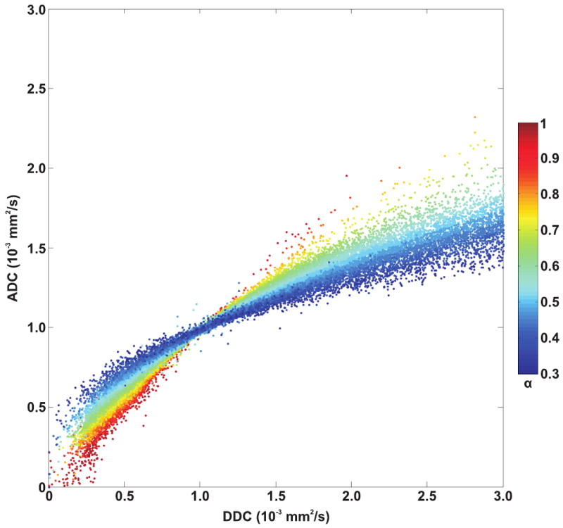
Scatterplot with voxel-based tumor DDCs (x-axis) against ADCs (y-axis), as a function of α value (colorized). ADCs appear to agree well with DDCs at approximately 1.0 × 10^-3 mm²/s and in any case α values are close to 1. However, as α values decrease, ADCs appear to be higher than DDCs at DDCs < 1.0 × 10^-3 mm²/s, whereas ADCs appear to be lower than DDCs at DDCs > 1.0 × 10^-3 mm²/s.

Figure 4.

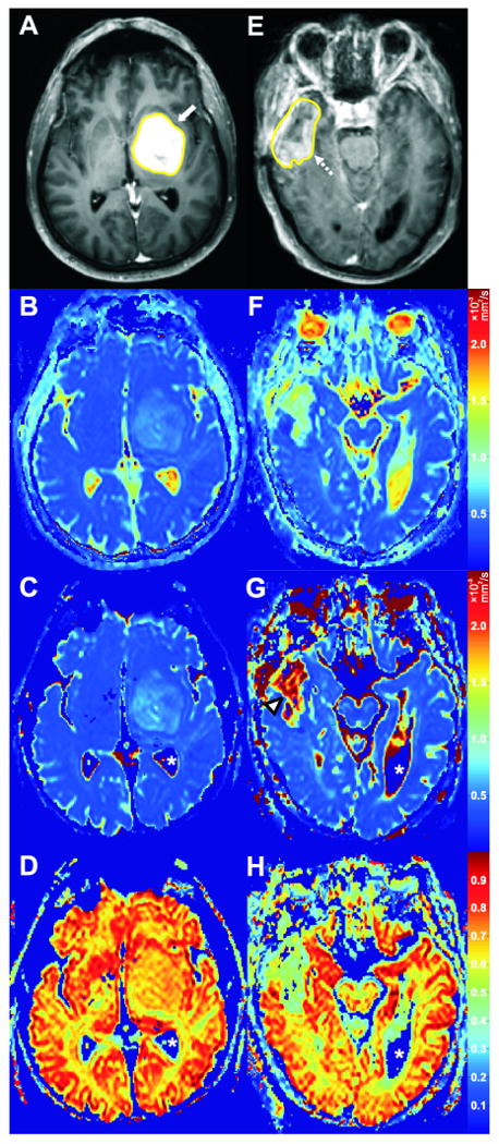
Two cases with good and poor agreement between ADC and DDC, respectively. Case 7 (Table 1); a 56-year-old male with a high-grade glioma (WHO grade IV) in the left frontal and temporal lobes (A-D). Axial post-gadolinium T1-weighted image with tumor VOI (A) clearly shows the enhancing tumor (white arrow). ADC, DDC, and α value of the tumor on corresponding axial ADC (B), DDC (C), and α (D) maps were 1.17 × 10^-3 mm²/s, 1.13 × 10^-3 mm²/s, and 0.68, respectively. The relatively good agreement between tumor ADC and DDC, and the relatively high α value of this tumor are well visualized (B, C, D). Case 9 (Table 1); a 69-year-old male with a high-grade glioma (WHO grade IV) in the right temporal lobe (E-F). Axial post-gadolinium T1-weighted image with tumor VOI (E) shows the enhancing part of the tumor (dashed arrow). ADC, DDC, and α value of the tumor on corresponding axial ADC (F), DDC (G), and α (H) maps were 1.45 × 10^-3 mm²/s, 2.41 × 10^-3 mm²/s, and 0.42, respectively. The poor agreement between tumor ADC and DDC is well visualized (F, G), with DDC being considerably higher (G, arrowhead). The relatively low α value of this tumor is also well visualized (H). It should be emphasized that α maps are completely different from ADC or DDC maps, because the former show intravoxel diffusion heterogeneity of tissues whereas the latter can only provide information on the intervoxel diffusion heterogeneity of tissues. Also note that the apparent “zero” DDCs and α values of the cerebrospinal fluid (C, D, G, H, white asterisks) are only a result of noise thresholding – these pixels were not included in the analyses.

Discussion

DWI allows the cellularity of tumors to be assessed noninvasively since cellular and sub-cellular elements impede water mobility, thus cellular-dense regions exhibit low ADC relative to necrotic and highly edematous tissues (1). By directly comparing ADCs of brain tumors with histological samples, several investigators (13-16) indeed showed that the ADC is inversely proportional to the cellular density, which may be helpful in brain tumor characterization. Other potential applications of DWI and ADC measurements lie in better tumor delineation, in the differentiation between radiation-induced necrosis and tumor recurrence, and in the early assessment of the effectiveness of radiation and/or chemotherapy (1, 17). At present, evidence of the effectiveness of DWI regarding brain tumor characterization, tumor delineation, and differentiation between radiation-induced necrosis and tumor recurrence is either conflicting or scarce (1), while a voxel-based quantitative DWI approach (currently referred to as parametric response mapping of diffusion) has recently shown promise as an early predictor of treatment response and survival in patients with high-grade gliomas (18, 19).

The ADC is the most commonly used measure of diffusion in clinical practice. Moreover, the choice of b-values 0 and 1000 s/mm² is probably the most widely used to generate ADC maps of the brain (9, 10). This protocol is well established and has led to a large published base of material. The DDC measurement, however, requires more than two b-values acquired over a relatively wide b-value range in order to illicit multi-exponential decay features, thus to date there is only limited published material on use of the stretched-exponential model applied to human gliomas. One can consider the DDC as a weighted sum over a distribution of ADCs that comprise the multi-exponential decay properties, and thus represents a more accurate depiction of diffusion in the presence of multiexponential decay (5, 7, 8). The motivation for this study was to determine the degree of agreement between the well-established “standard” ADC and the potentially more accurate DDC, albeit more difficult to generate. Moreover, the present study sought to determine the circumstance where ADC and DDC disagree. The present results indicate that low ADCs agree reasonably well with DDCs in high-grade gliomas. However, assuming the DDC to be a more accurate estimate of the average diffusion rate, higher ADCs may underestimate the amount of diffusion in high-grade gliomas (i.e., DDCs are even higher). A previous animal model of glioma also noticed lower tumor ADCs relative to tumor DDCs (7), although this finding was not clearly explained and may not (quantitatively) apply to human high-grade gliomas.

The findings of the present study can be explained by the stretched-exponential model itself and the biological properties of high-grade gliomas. First, reviewing equations [1] (S(b)/S₀ = exp (-b × ADC)) and [4] (S(b)/S₀ = exp (-(b × DDC)^α)) shows that when b × DDC = 1 (regardless of α value) or when α = 1 (regardless of b value or DDC), DDC ≈ ADC. However, if b × DDC > 1, a decrease in the α value results in a decrease in signal attenuation as a function of b-value. If b × DDC < 1, the opposite effect occurs, such that low α values result in a relatively fast signal decay. Thus, b × DDC = 1 delineates “high” and “low” ranges of decay rates (5, 7, 8). Next, consider the case where two fixed b-values are used for calculating the ADC. From equations [1] and [4], the following equation can be derived:

$$\mathit{\text{ADC}}=b^{\alpha -\mathit{1}}\times DD{C}^{\alpha }$$ [5]

If b × DDC = 1, DDC ≈ ADC, regardless of the α value (note that this occurs at a DDC or ADC of 1 × 10^-3 mm²/s when using a b-value of 1000 s/mm²) (Figure 4 5). If α < 1, and b × DDC > 1, ADC will be lower than DDC (Figure 4). In contrast, if α < 1, and b × DDC < 1, ADC will be higher than DDC (Figure 5). Also recall that the higher the α value, the better ADC and DDC should agree (note, at the mono-exponential extreme α = 1, thus DDC = ADC). The present data support this since at higher α values the observed ADCs and DDCs of high-grade gliomas are in reasonable agreement (i.e., data points are close to the line of unity in Figure 1, and low difference between ADC and DDC in Figure 2), and this agreement occurs in the low ADC regime. In contrast, the lower the α value the poorer the agreement between ADC and DDC; and this divergence is observed at higher ADCs or DDCs in high-grade gliomas. It should be noted that highly necrotic/cystic elements of tumor were eliminated from analysis in this study by the noise-threshold filter in the stretched-exponential fitting routine. As such our results pertain to the cellular components of tumor and exclude cyst. Cystic tissues commonly have an ADC > 2.5 × 10^-3 mm²/s, however such high water mobility tissues did not retain adequate signal at b=4000 s/mm² for stretched-exponential fitting thus were rejected. If SNR was not a limitation, simple cyst predominantly composed of water should appear as mono-exponential (α≈1) with high ADC≈DDC. To support these findings, a water phantom with varying local temperatures was scanned, and a good agreement between ADC and DDC, at a reasonably wide range of ADCs, was found. The highest diffusion value (in 10^-3 mm²/s) achieved in the phantom before signal dropped below the noise threshold was ADC = 2.01 ± 0.04 with a corresponding DDC = 2.02 ± 0.05, and an α = 0.99 ± 0.07. Therefore, we believe the disagreement between ADC and DDC in glioma in the high ADC-DDC regime is a direct result of complex diffusion in biological system and not an artifact of fitting the stretched-exponential model to the data. Regardless of its exact biological meaning, its clinical consequence is that although low ADCs will agree fairly well to DDCs, high ADCs will be in poor agreement with DDCs and may underestimate diffusion values (assuming the DDC to be a more accurate measure of the average diffusion rate); this may lead to incorrect lesion characterization (e.g. underestimation of the amount of necrosis) and may render studies in which the ADC is used for assessing response to therapy less sensitive for the detection of changes in diffusion.

Figure 5.

Graph with DDC (x-axis) against ADC (y-axis), with varying α values, according to equation [5] (ADC = b^α-1× DDC^α). B-values of 0 and 1000 s/mm² are used to calculate the ADC. If b × DDC = 1, DDC ≈ ADC, regardless of the α value (note that this occurs at a DDC or ADC of 1000 s/mm² when using a b-value of 1000 s/mm²). If α < 1, and b × DDC > 1, ADC will be lower than DDC. In contrast, if α < 1, and b × DDC < 1, ADC will be higher than DDC. Also recall that the higher the α value, the better ADC and DDC agree (note, at the mono-exponential extreme α = 1, thus DDC = ADC).

In order to obtain ADCs that equal DDCs, it has been proposed to optimize the b-value for each tissue, such that b × DDC = 1 (5). This may be useful, for instance, in localizing a region of cytotoxic edema following the onset of stroke (5). However, in contrast to acute ischemic stroke, high-grade gliomas encompass a wide range of DDCs (0.68 to 2.80 × 10^-3 mm²/s in the present study), and optimizing the b-value before scanning seems to be impractical. Nevertheless, lower b-values (i.e. < 1000 s/mm²) may be more useful to quantify diffusion by means of the ADC in high-grade gliomas. Alternatively, when aiming to obtain more precise diffusion quantification or increasing sensitivity for the detection of changes in diffusion, it may be necessary to obtain a DDC instead of an ADC.

A disadvantage of using the DDC is the need to add a few more b-values (>1000 s/mm²) to a conventional DWI sequence (usually performed at b-values of 0 and 1000 s/mm²), which prolongs examination time. Furthermore, fitting the stretched-exponential model to the DWI data to obtain DDC maps takes extra post-processing time, and is typically not included in clinical software packages. Furthermore, it should be noted that the present study only included high-grade gliomas, and it is still unclear if, and to what extent, ADCs and DDCs of low-grade gliomas or other brain tumors agree. Perhaps low-grade gliomas exhibit less intravoxel diffusion heterogeneity than high-grade gliomas because of less histological heterogeneity of the former. Consequently, ADC and DDC measurements may be in better agreement in low-grade gliomas than in high-grade gliomas due to the more mono-exponential signal decay of the former (i.e. α values close to 1). However, this issue remains speculative and further research is needed. Another study limitation is that although the DDC is assumed to represent a more accurate depiction of diffusion than the ADC in the presence of multiexponential signal decay (5, 7, 8), this has not been confirmed yet by in vivo studies with histopathological correlation.

In conclusion, under the assumption that the stretched-exponential model provides a more accurate estimate of the average diffusion rate than the mono-exponential model, our results suggest that for a little diffusion attenuation the mono-exponential fit works rather well for quantifying diffusion in high-grade gliomas, whereas it works less well for a greater degree of diffusion attenuation.

References

- 1.Provenzale JM, Mukundan S, Barboriak DP. Diffusion-weighted and perfusion MR imaging for brain tumor characterization and assessment of treatment response. Radiology. 2006;239:632–649. doi: 10.1148/radiol.2393042031. [DOI] [PubMed] [Google Scholar]
- 2.Bammer R. Basic principles of diffusion-weighted imaging. Eur J Radiol. 2003;45:169–184. doi: 10.1016/s0720-048x(02)00303-0. [DOI] [PubMed] [Google Scholar]
- 3.Sotak CH. Nuclear magnetic resonance (NMR) measurement of the apparent diffusion coefficient (ADC) of tissue water and its relationship to cell volume changes in pathological states. Neurochem Int. 2004;45:569–582. doi: 10.1016/j.neuint.2003.11.010. [DOI] [PubMed] [Google Scholar]
- 4.Maier SE, Bogner P, Bajzik G, et al. Normal brain and brain tumor: multicomponent apparent diffusion coefficient line scan imaging. Radiology. 2001;219:842–849. doi: 10.1148/radiology.219.3.r01jn02842. [DOI] [PubMed] [Google Scholar]
- 5.Bennett KM, Schmainda KM, Bennett RT, Rowe DB, Lu H, Hyde JS. Characterization of continuously distributed cortical water diffusion rates with a stretched-exponential model. Magn Reson Med. 2003;50:727–734. doi: 10.1002/mrm.10581. [DOI] [PubMed] [Google Scholar]
- 6.Lee JH, Springer CS., Jr Effects of equilibrium exchange on diffusion-weighted NMR signals: the diffusigraphic “shutter-speed”. Magn Reson Med. 2003;49:450–458. doi: 10.1002/mrm.10402. [DOI] [PubMed] [Google Scholar]
- 7.Bennett KM, Hyde JS, Rand SD, et al. Intravoxel distribution of DWI decay rates reveals C6 glioma invasion in rat brain. Magn Reson Med. 2004;52:994–1004. doi: 10.1002/mrm.20286. [DOI] [PubMed] [Google Scholar]
- 8.Bennett KM, Hyde JS, Schmainda KM. Water diffusion heterogeneity index in the human brain is insensitive to the orientation of applied magnetic field gradients. Magn Reson Med. 2006;56:235–239. doi: 10.1002/mrm.20960. [DOI] [PubMed] [Google Scholar]
- 9.Al-Okaili RN, Krejza J, Woo JH, et al. Intraaxial brain masses: MR imaging-based diagnostic strategy – initial experience. Radiology. 2007;243:539–550. doi: 10.1148/radiol.2432060493. [DOI] [PubMed] [Google Scholar]
- 10.Padhani AR, Liu G, Mu-Koh D, et al. Diffusion-weighted magnetic resonance imaging as a cancer biomarker: consensus and recommendations. Neoplasia. 2009;11:102–125. doi: 10.1593/neo.81328. [DOI] [PMC free article] [PubMed] [Google Scholar]
- 11.Meyer CR, Boes JL, Kim B, et al. Demonstration of accuracy and clinical versatility of mutual information for automatic multimodality image fusion using affine and thin-plate spline warped geometric deformations. Med Image Anal. 1997;1:195–206. doi: 10.1016/s1361-8415(97)85010-4. [DOI] [PubMed] [Google Scholar]
- 12.Bland JM, Altman DG. Statistical methods for assessing agreement between two methods of clinical measurement. Lancet. 1986;1:307–310. [PubMed] [Google Scholar]
- 13.Sugahara T, Korogi Y, Kochi M, et al. Usefulness of diffusion-weighted MRI with echo-planar technique in the evaluation of cellularity in gliomas. J Magn Reson Imaging. 1999;9:53–60. doi: 10.1002/(sici)1522-2586(199901)9:1<53::aid-jmri7>3.0.co;2-2. [DOI] [PubMed] [Google Scholar]
- 14.Chenevert TL, Stegman LD, Taylor JM, et al. Diffusion magnetic resonance imaging: an early surrogate marker of therapeutic efficacy in brain tumors. J Natl Cancer Inst. 2000;92:2029–2036. doi: 10.1093/jnci/92.24.2029. [DOI] [PubMed] [Google Scholar]
- 15.Guo AC, Cummings TJ, Dash RC, Provenzale JM. Lymphomas and high-grade astrocytomas: comparison of water diffusibility and histologic characteristics. Radiology. 2002;224:177–183. doi: 10.1148/radiol.2241010637. [DOI] [PubMed] [Google Scholar]
- 16.Lyng H, Haraldseth O, Rofstad EK. Measurement of cell density and necrotic fraction in human melanoma xenografts by diffusion weighted magnetic resonance imaging. Magn Reson Med. 2000;43:828–836. doi: 10.1002/1522-2594(200006)43:6<828::aid-mrm8>3.0.co;2-p. [DOI] [PubMed] [Google Scholar]
- 17.Zhao M, Pipe JG, Bonnett J, Evelhoch JL. Early detection of treatment response by diffusion-weighted 1H-NMR spectroscopy in a murine tumour in vivo. Br J Cancer. 1996;73:61–64. doi: 10.1038/bjc.1996.11. [DOI] [PMC free article] [PubMed] [Google Scholar]
- 18.Hamstra DA, Galbán CJ, Meyer CR, et al. Functional diffusion map as an early imaging biomarker for high-grade glioma: correlation with conventional radiologic response and overall survival. J Clin Oncol. 2008;26:3387–3394. doi: 10.1200/JCO.2007.15.2363. [DOI] [PMC free article] [PubMed] [Google Scholar]
- 19.Hamstra DA, Rehemtulla A, Ross BD. Diffusion magnetic resonance imaging: a biomarker for treatment response in oncology. J Clin Oncol. 2007;25:4104–4109. doi: 10.1200/JCO.2007.11.9610. [DOI] [PubMed] [Google Scholar]