Quantitative Analysis of Arterial Spin Labeling FMRI Data Using a General Linear Model

Abstract

Arterial Spin Labeling techniques can yield quantitative measures of perfusion by fitting a kinetic model to difference images (tagged-control). Because of the noisy nature of the difference images investigators typically average a large number of tagged versus control difference measurements over long periods of time. This averaging requires that the perfusion signal be at a steady state and not at the transitions between active and baseline states in order to quantitatively estimate activation induced perfusion. This can be an impediment for FMRI task experiments. In this work, we introduce a general linear model (GLM) that specifies BOLD effects and ASL modulation effects and translate them into meaningful, quantitative measures of perfusion by using standard tracer kinetic models. We show that there is a strong association between the perfusion values using our GLM method and the traditional subtraction method, but that our GLM method is more robust to noise.

Introduction

Arterial Spin Labeling techniques can yield quantitative measures of perfusion by fitting a kinetic model to tagged versus control difference images. The noisy nature of the difference images forces investigators to average a large number of tagged versus control difference measurements over long periods of time. This averaging requires that the perfusion signal be at a steady state and not at the transitions between active and baseline states in order to quantitatively estimate activation induced perfusion. While this is not an impediment for studies of baseline brain function, it limits the scope of FMRI task experiments to baseline perfusion measurements or long block designs (Carmichael et al., 2008; Detre et al., 2009; Lui et al., 2009; Xu et al., 2007; Dai et al., 2009; Kim et al., 2006; Restom et al., 2007). To make matters worse, the inherently low temporal resolution of ASL signals makes this approach impractical, as few data points are available at each condition. Another challenge to quantification of perfusion from ASL time series using kinetic models - for example, see (Williams et al., 1992; Alsop and Detre, 1996; Wang et al., 2002) - arises because the noise in the input images accumulates and becomes amplified by the image operations. Again, while this is not so problematic for computation of a baseline perfusion image obtained from a large number of averages, it makes quantification of dynamic changes in perfusion time series quite challenging. It is highly desirable to measure the change in perfusion due to an effect of interest in a wide range of activation paradigms including blocked and event-related designs. It is indeed technically possible to collect event-related ASL data (Hernandez-Garcia et al., 2004; Liu et al., 2002; Miller et al., 2001) but, to our knowledge, there are no cognitive studies utilizing quantitative ASL that involve event-related designs, or larger design matrices that account for more than two effects of interest.

In this work, we introduce a different solution to this problem: to estimate the parameters of a general linear model (GLM) that specifies BOLD effects and ASL modulation effects and translate them into meaningful, quantitative measures of perfusion by using standard tracer kinetic models. Indeed, Liu et al. introduced an elegant signal processing model that captured BOLD and perfusion effects simultaneously in ASL data and the consequences of differencing those data (Liu et al., 2005). Mumford et al. showed that Generalized Least Squares estimation yielded optimally efficient parameter estimates from unsubtracted ASL data for the purpose of statistical mapping (Mumford et al., 2006) and, similarly, Woolrich et al. used a Bayesian approach to make statistical inferences on significance of perfusion and T₂* effects from dual-echo, ASL data (Woolrich et al., 2006). While these parameter estimates of ASL time series data are being used to calculate statistical measures of significance, they are not utilized to their full extent, as they contain valuable information about perfusion. The method presented here takes the next step: physiologically meaningful quantification of those parameter estimates. This method is based on the simple realization that the difference images used in ASL quantitative models have a direct relationship to the parameter estimates in general linear model estimation.

Theory

Let us consider an ASL FMRI experiment with a baseline condition and a single activation condition with tag and control ASL images acquired in each. One such experiment can be characterized by a linear model, as previously described (Mumford et al., 2006). For example, let y_t be the time course (a vector) of image intensity at a particular voxel obtained from an ASL experiment. In Fig. 1 are the regressors of a simple ASL design matrix representing the linear model

Fig. 1.

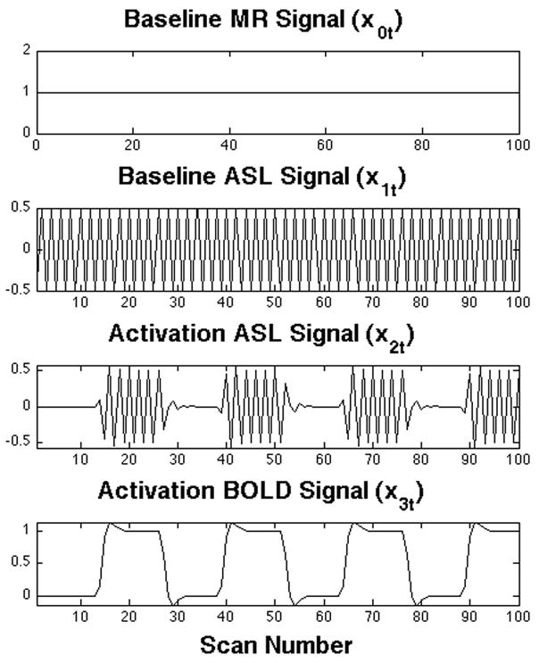
Simple ASL design matrix. Each plot represents one column (regressor) of the design matrix and its coefficient parameter (β). The first regressor indicates the baseline state signal, or spin density. The second regressor describes the baseline difference between control and tagged images (ΔM), is indicative of baseline perfusion. The third regressor describes ΔM changes due to activation. The fourth regressor describes residual BOLD effect changes.

$$y_t={\beta }_0+{\beta }_1{x}_{1t}+{\beta }_2{x}_{2t}+{\beta }_3{x}_{3t}+{\epsilon }_t$$ (1)

for time t=1,…,n. The first regressor, the baseline vector x_0t,=1 and its coefficient parameter, the scalar β ₀, indicate the baseline signal, and can be interpreted as a measure of spin density. The second regressor x_1t describes the baseline difference between control and tagged images (ΔM) and thus its amplitude, β ₁, is indicative of baseline perfusion. The third regressor x_2t with its regression coefficient β ₂ describes differences between control and tagged images (ΔM) due to activation, and the fourth regressor x_3t with its regression coefficient β ₃ describes the BOLD effect changes. By realizing that the amplitude of the oscillation β ₂ induced by the ASL scheme corresponds to the difference between control and tagged images, perfusion can be computed dynamically by translating the coefficient parameter estimates of the oscillations into the appropriate control-tag differences. Quantification of perfusion effects in continuous ASL data without background suppression can be done directly by adapting a kinetic model (e.g., see Eq. (A1) in (Wang et al., 2002))

$$f_{\mathit{effect},t}=\frac{\lambda ·R_{1\mathit{app}}·{\widehat{\beta }}_{\mathit{effect}}}{\left(\frac{{\widehat{\beta }}_0}{1-e^{-TR/T_1}}\right)·2·\alpha ·e^{-\delta ·R_{1a}}·\left(e^{(\delta -w)·R_{1\mathit{app}}}-e^{(\delta -\tau -w)·R_{1\mathit{app}}}\right)}·x_{\mathit{effect},t}$$ (2)

where f̂_effect,t is the estimated perfusion change due to the effect of interest, α is the inversion efficiency, x_effect,t is the regressor for the effect at time t, β̂_effect is the coefficient parameter estimate of the regressor representing the effect of interest (for example, the amplitude of the perfusion changes due to activation in the above model are captured by β₂), β̂ ₀ is the baseline state signal (T₁-weighted spin density), λ is the blood brain partition coefficient, R₁, R_1a, R_1app are the longitudinal relaxation rates of arterial blood, tissue, and tissue in the presence of perfusion. The term δ is the arterial transit time, while TR, w, and τ are repetition time, post labeling delay, and labeling duration. As previously noted (Wang et al., 2002), when long post-inversion delays (w) are used, the equation becomes insensitive to changes in arterial transit time. We note that the sign of β̂_effect can be positive or negative depending on the acquisition order of the control and tagged pairs.

Generalized Least Squares estimation yields estimates of the linear model’s parameters and their variances. Thus, the same relationship can be used to derive the standard deviation of the estimates in perfusion units. In order to calculate the variance of the estimated perfusion effects, we propagate the errors of the relevant coefficient parameter estimates through the kinetic model. Propagation of error can be calculated in a straightforward way from the partial derivatives of the model relative to the coefficient parameters of interest (Bevington and Robinson, 2003) as follows

$$\frac{\partial {\widehat{f}}_{\mathit{effect},t}}{\partial {\widehat{\beta }}_0}=-\frac{\lambda ·\left(x_{\mathit{effect},t}{\widehat{\beta }}_{\mathit{effect}}\right)·R_{1\mathit{app}}}{\left(\frac{{{\widehat{\beta }}_0}^2}{1-e^{-TR·R_1}}\right)·2·\alpha ·e^{-\delta ·R_{1a}}\left(e^{(\delta -w)·R_{1\mathit{app}}}-e^{(\delta -\tau -w)·R_{1\mathit{app}}}\right)}$$ (3)

$$\frac{\partial {\widehat{f}}_{\mathit{effect},t}}{\partial {\widehat{\beta }}_{\mathit{effect}}}=\frac{\lambda ·x_{\mathit{effect},t}·R_{1\mathit{app}}}{\left(\frac{{\widehat{\beta }}_0}{1-e^{-TR·R_1}}\right)·2·\alpha ·e^{-\delta ·R_{1a}}\left(e^{(\delta -w)·R_{1\mathit{app}}}-e^{(\delta -\tau -w)·R_{1\mathit{app}}}\right)}.$$ (4)

Hence the variance of the perfusion estimate in Eq. (2) due to the variance in the parameter estimates can be calculated by using the partial derivatives in Eq. (3) and Eq. (4) and given by

$${\widehat{\sigma }}^2={\widehat{\sigma }}_{{\widehat{\beta }}_0}^2{\left(\frac{\partial {\widehat{f}}_{\mathit{effect},t}}{\partial {\widehat{\beta }}_0}\right)}^2+{\widehat{\sigma }}_{{\widehat{\beta }}_{\mathit{effect}}}^2{\left(\frac{\partial {\widehat{f}}_{\mathit{effect},t}}{\partial {\widehat{\beta }}_{\mathit{effect}}}\right)}^2+2·\mathit{COV}({\widehat{\beta }}_0,{\widehat{\beta }}_{\mathit{effect}})·\left(\frac{\partial {\widehat{f}}_{\mathit{effect},t}}{\partial {\widehat{\beta }}_0}\right)·\left(\frac{\partial {\widehat{f}}_{\mathit{effect},t}}{\partial {\widehat{\beta }}_{\mathit{effect}}}\right).$$ (5)

Statistical significance (e.g., a t-score) in perfusion changes due to the effect of interest f_effect,t can be determined by dividing the estimated f̂_effect,t in Eq. (2) by the square root of the estimated variance of the effect of interest ${\sigma }_{{\beta }_{\mathit{effect}}}^2$ in Eq. (5). Statistically significant changes in perfusion can also be estimated using the traditional method that averages together the pairwise subtractions collected during baseline and activation then using those values in a kinetic model as in Eq. (2). The variance of perfusion can also be computed during intervals corresponding to baseline and activation periods. In our GLM method we will simplify the variance of our perfusion estimate in Eq. (5) by neglecting the covariance between our baseline state signal and the coefficient for the effect of interest.

We have previously shown that Generalized Least Squares estimation of unsubtracted data yields more efficient estimates than Ordinary Least Squares estimation of differenced data, while accounting for autocorrelated noise (Mumford et al., 2006). This approach also enables us to estimate BOLD and ASL effects simultaneously, as their corresponding regressors are uncorrelated. However, differencing schemes reduce the degree of autocorrelation dramatically in ASL data (Aguirre et al., 2002; Liu and Wong, 2005) and are widely used. While we choose to model both the ASL and BOLD effects in un-differenced data, the method described here can also be used with differenced data, as long as the design matrix is constructed carefully to reflect the differencing scheme.

Methods

Simulated data

ASL time courses acquired during a simple blocked design paradigm were synthesized, and white Gaussian noise was added to them. The paradigm consisted of five 50 second periods of baseline alternating with five 50 second periods of activation. A General Linear Model of the paradigm was built by generating regressors for: (1) the signal baseline, (2) the baseline perfusion modulated by alternating control and tagged scans, (3) the activation perfusion modulated by alternating control and tagged scans and (4) signal increases due to BOLD effects during activation. For more detail on this approach, please see (Mumford et al., 2006). The design matrix for the experimental paradigm is displayed in Fig. 1 where the columns are plotted with time on the horizontal axis. Relevant acquisition parameters were as follows: TR = 4 s, tagging time = 2 s, post inversion delay = 1.5 s, transit time = 1.5 s. The true coefficient values were 10000, 50, 20, 50 arbitrary units (au). When using the model in (Wang et al., 2002), these oscillations correspond to baseline and activation perfusions of 39.3 and 55.0 ml/min/100 g. Fifty time courses were computed with the variance of the added noise varying from 0 to 500 au² in steps of 10 au². The T₁ relaxation times of tissue and blood were assumed to be 1400 and 1600 ms, respectively (Stanisz et al., 2005; Lu et al., 2004).

Perfusion parameter estimates and their corresponding variances were calculated from the synthetic ASL signals using the GLM technique described in this manuscript. Perfusion time courses were also computed from the same synthetic signals by a standard kinetic model that uses pairwise subtraction of the ASL signal. For the standard synthetic model, eight points from every “baseline” and “activation” interval as shown in Fig. 2 were used to calculate the mean and variance of perfusion during baseline and activation. Data acquired during the transitions between baseline and activation were excluded, as the dynamically changing perfusion would significantly affect the estimates of the baseline and activation periods. The mean baseline perfusion obtained from the traditional methods was compared to the baseline perfusion parameter obtained from the GLM estimation. Likewise, the mean perfusion during activation was compared to the activation perfusion parameter estimates. Variances of the baseline and activation perfusion values were compared to the variance of the perfusion parameter estimates.

Fig. 2.

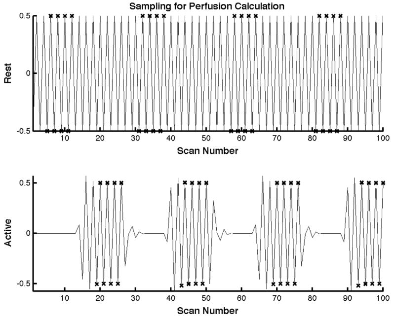
Samples used for perfusion estimation using the traditional method are shown for one block of the task. The top and bottom plots represent the baseline and active state ASL signals respectively. Samples close to the transition from baseline to active and vise versa were not used for estimation. The samples used for computation of the mean active and baseline state perfusions are marked with an × respectively.

Experimental Data

The technique was also demonstrated experimentally in a simple stimulation paradigm, as follows. Visual stimulation was performed by showing the subjects a circular, flashing, checkerboard pattern. The subjects were instructed to tap their thumbs against their fingers as fast as they could while the flashing checkerboard was shown to them and to remain still with their eyes open otherwise. The stimulation paradigm consisted of four periods of baseline (50 seconds long) followed by four periods of stimulation (50 seconds long). Scanning was carried out on a 3T General Electric Signa MRI scanner (Waukesha, WI). Arterial Spin Labeling images were collected during the paradigm using a pseudo CASL (Dai et al., 2008) sequence (TR/TE=4000/3 ms, tagging time=2000 ms, post inversion delay=1500 ms, matrix=64×64, 8 slices, thickness = 6 mm, gradient-echo spiral acquisition).

A General Linear Model of the paradigm was built in the same fashion as in the simulation and is displayed in Fig. 1 where the columns are plotted with time on the horizontal axis. A GLM analysis of prewhitened data was used to estimate regression coefficients and to identify significantly active voxels (Z>3). Time courses were extracted from volumes of interest defined by supra-threshold voxels within a 12 mm diameter sphere in the visual and motor cortices.

Perfusion maps were computed from the parameter estimates of the GLM, as described in the theory section, and assuming the following physiological parameters: Transit time (δ)=1500 ms, inv. Efficiency (α) = 0.85, Gray Mater T₁ = 1400 ms, Arterial T₁ = 1600 ms (Stanisz et al., 2005) (Lu et al., 2004).

As with the simulated data, perfusion for the experimental data was also computed from the extracted time courses using the more traditional approach of averaging together the pairwise subtractions collected during baseline and activation and using those values in a kinetic model. The mean and variance of perfusion were computed during intervals corresponding to baseline and activation periods. Subtraction pairs corresponding to the transition periods between baseline and activation (16 seconds) were excluded from the calculations, as the dynamically changing perfusion would significantly affect the estimates of the baseline and activation periods.

Results

Simulated Data

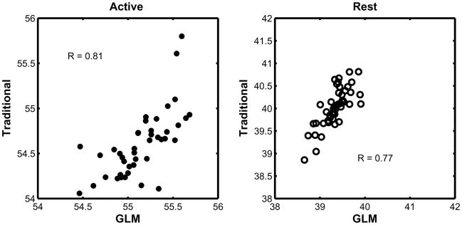
Correlation plots between the mean perfusion measurements obtained from both methods at the highest noise level can be seen in Fig. 3. The correlation coefficients were 0.81 and 0.77 during activation and baseline, respectively, and the slopes of the fit were 1.01 and 0.98. The estimates of the perfusion parameters from the GLM showed good agreement with the perfusion estimates obtained using the traditional approach. Both methods underestimated the baseline perfusion by less than 8% (traditional) and 5% (GLM). The GLM method’s error is symmetric about the true value, while the traditional method appears to have underestimated it by less than 2%.

Fig. 3.

Correlation plots between the perfusion values obtained using the traditional method and the proposed GLM method. The relationship between the two methods is clearly linear but the GLM method yields higher perfusion values than the traditional method, since the estimated coefficient in the GLM method corresponds to the peak perfusion, rather than the plateau.

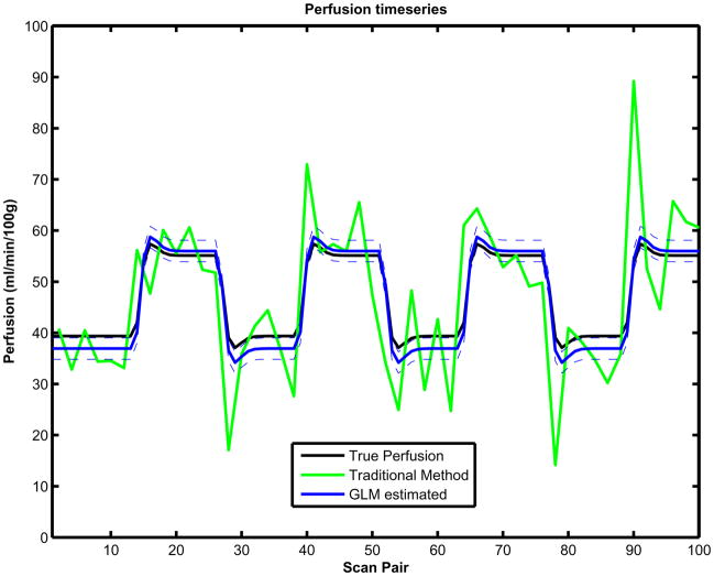
The ASL GLM model in Eq. (1) was fit to the simulated time course data and the perfusion was estimated dynamically using Eq. (2) as well as the variance of the perfusion using Eq. (5). The perfusion was also estimated using the traditional method. The GLM-estimated perfusion time course from a sample simulated ASL time course using Eq. (2) is presented in Fig. 4 along with a one standard deviation confidence band. The corresponding perfusion time course estimated using the traditional method (green) and the true temporal perfusion time course using the true GLM regression coefficients and Eq. (2) are also presented (black). The GLM coefficient parameter estimates of all the regressors from this sample time course were (9999, 50.7, 22.7, 50.8) au. The corresponding GLM parameter standard deviation estimates from Eq. (5) were 0.93, 1.34, 1.88 and 0.94 au. These GLM parameter estimates yielded baseline and activation perfusions of 39.8 and 57.6 ml/min/100 g with associated standard deviations of 1.06 and 1.50 ml/min/100 g. The traditional approach yielded baseline and activation perfusions of 37.9 and 54.6 ml/min/100 g with associated variances of 34.2 and 45 (ml/min/100 g)². For comparison, recall that the true coefficient values were set to 10000, 50, 20, 50 au, corresponding to perfusion levels of 39.3 and 55.0 ml/min/100 g.

Fig. 4.

Estimated temporal perfusion plots for simulated data using the GLM are indicated by the solid blue line. Traditional measurements of the time series are indicated in green, and the true perfusion value is denoted by the solid black line. Standard Deviations of perfusion calculated using the GLM approach are indicated by the dashed blue line.

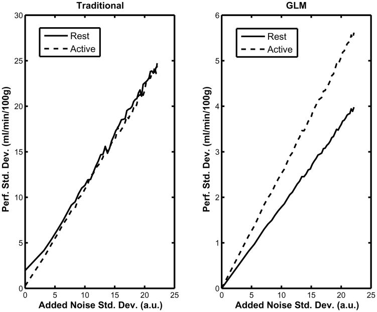
The behavior of the variance of the estimates in each method can be seen in Fig. 5. As Fig. 5 shows, the measured variance increases linearly with the variance of the added noise vector in both the traditional and the GLM approach. Note in Fig. 5 (left) that the baseline perfusion variance in the traditional approach does not go to zero when the variance of the added noise was zero. The baseline and active variance estimates were affected linearly by the noise level in the data using the traditional approach. Additionally there was an apparent shift in the intercept of approximately 2 and 4 (ml/min/100 g)². This shift was due to the slow settling time of the perfusion function results in significant variation of the extracted signal, even in the absence of noise. While more “unsettled” points can be excluded from the calculation, completely removing them severely reduces the amount of data available for estimation of the perfusion. Fig. 5 (right) shows that the relationship between the noise variance and variance of the parameters is also linear when using our GLM approach. However, the slope is dramatically smaller than in the traditional approach. Note that when the variance of the noise increases up to 500 au², the variances of the parameter estimates are approximately 30 and 15 (ml/min/100 g)² in the GLM approach, rather than 600 (ml/min/100 g)² in the traditional approach. Also note that the activation parameter variance is more sensitive to the noise than the baseline one.

Fig. 5.

The left panel shows the variance of the perfusion values calculated using the traditional method during baseline and activation as a function of the noise level added to the synthetic data. The right panel shows the variance of the perfusion estimates computed using to the proposed GLM method also as a function of the noise level added to the synthetic data. The data are expressed in arbitrary units (au).

Experimental Data

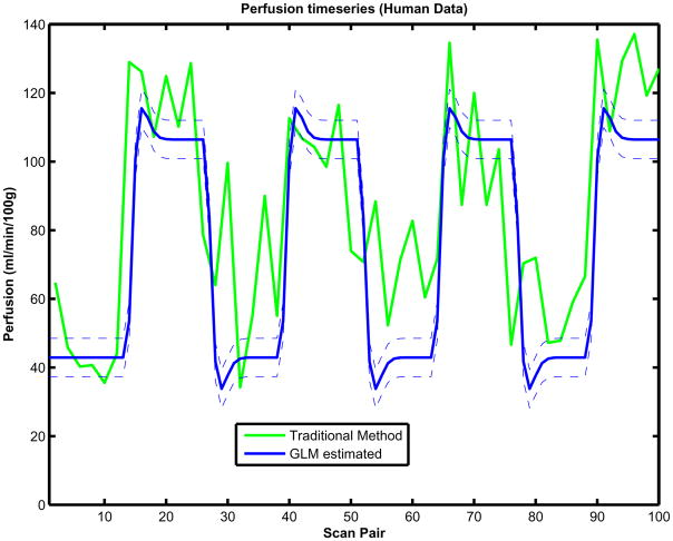
For the experimental data, the ASL GLM model in Eq. (1) was also fit to the time course data and the perfusion was estimated dynamically using Eq. (2) as well as the variance of the perfusion using Eq. (5). Perfusion time courses were also estimated using the traditional method. A GLM-estimated perfusion time course from a visual cortex ROI on a representative subject is presented in Fig. 6 along with a one standard deviation confidence band. The corresponding perfusion time course estimated using the traditional method are also presented (green). The GLM parameter estimates of all the regressors from this sample time course were (2411.5, 13.1, 19.5, 6.3) au. The corresponding GLM parameter standard deviations were 19.6, 13.9 and 22.0 au. These GLM parameter estimates yielded baseline and activation perfusions of 42.9 and 106.4 ml/min/100 g with associated standard deviations of 2.79 and 3.94 ml/min/100 g The traditional approach yielded baseline and activation perfusions of 57.3 and 109.2 ml/min/100g, with estimated standard deviations of 17.9 and 19.9 m;/min/100 g.

Fig. 6.

Estimated temporal perfusion plots for human data using the GLM (blue) approach and traditional (green). Variance of perfusion using the GLM approach (dashed thin line blue) are also included.

In Fig. 7 are the resulting perfusion estimate maps and their standard deviation for one subject displaying the corresponding changes due to activation in the motor and visual task. The underlay image shows the baseline perfusion. The overlaid maps show the changes in perfusion associated with the stimulation tasks. Fig. 7 (top left) presents the estimated differential perfusion using the GLM approach and Fig. 7 (bottom left) presents the estimated differential perfusion using the traditional subtraction. The color scales are in units of ml/min/100 g. Fig. 7 (top right) presents the variance of perfusion estimates using the GLM approach and Fig. 7 (bottom right) presents the standard deviation of perfusion estimates using the traditional subtraction method. The color scales are in units of ml/min/100 g. The underlay images depict the estimated variance of the baseline perfusion and the overlay maps depict the estimated variance of the activation perfusion. Note that they are thresholded such that only statistically significant (Z>3) increases in perfusion are shown. Those areas include the motor and visual cortices.

Fig. 7.

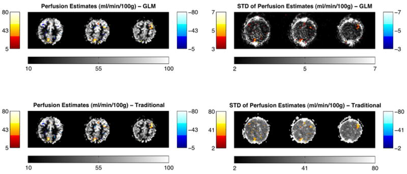
Resulting perfusion maps in one of the subjects using GLM approach (top left) and traditional subtraction approach (bottom left), showing the corresponding changes in perfusion due to activation in motor/visual task. As expected, significant increases in motor and visual cortices can be observed. The underlay image shows the estimate of baseline perfusion. The overlaid maps show the statistical changes in perfusion associated with the stimulation tasks. The color scales are in units of ml/min/100 g. The resulting standard deviation of perfusion estimates for one subject using the GLM approach (top right) and standard deviation of perfusion estimates using the traditional subtraction method (bottom right). The color scales are in units of ml/min/100 g.

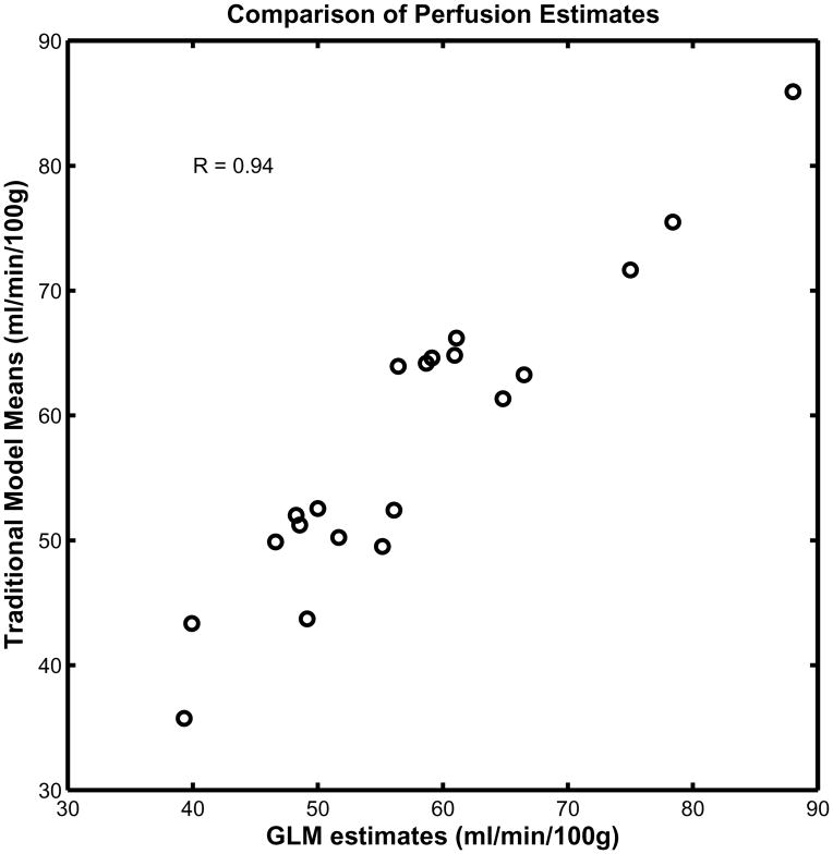
Fig. 8 is a scatter plot of the GLM perfusion estimates and the mean perfusion computed using the traditional method. The data used for this plot consist of the mean perfusion inside an active region of interest defined by a sphere with 12 mm diameter and Z score > 3 pooled from all subjects under both baseline and activation conditions.

Fig. 8.

Comparison of perfusion estimates using GLM and traditional approach: Scatter plot of perfusion in ROIs places on visual and motor cortices during baseline and activation for 5 subjects estimated using Traditional approach (y axis) versus GLM approach (x axis) is presented. As can be seen, there is a significant correlation between perfusion estimates of these two methods (r=0.94).

Discussion

In the GLM method we have presented, parameters of the kinetic model have been estimated along with their variances. From the parameter estimates and their variances, quantitative perfusion parameter maps can readily be generated. As shown in Figs. 4 and 5, perfusion time courses can also be obtained from the model and the parameter estimates. We showed that there is a good association between the perfusion values using our GLM method and the traditional subtraction method but that our GLM method is more robust to noise, can be used to estimate perfusion changes in wider array of experimental designs, and can estimate the entire temporal perfusion curve, given an accurate model.

While the perfusion levels being measured by the traditional and GLM methods are not identical, they are closely linked to each other. The GLM method produces estimates of the peak perfusion due to activation. The traditional method, on the other hand, computes the mean perfusion increase during the plateau of the activation, which accounts for discrepancies between the means and also for the larger variance of the activation perfusion. In a blocked design, these two quantities are more intimately linked, as evidenced by the tight correlation between the two methods displayed in Fig. 8.

It is crucial to realize that the variance estimates obtained from the GLM approach have a different meaning than those obtained by calculating the variance on a time course of perfusion measurements computed from pairwise subtractions. The former refers to the variance of a contrast of the estimates of a model’s parameters, while the later is strictly the variance of selected segments of the perfusion time course. The former utilizes the entire time course in relation to the experimental design matrix. The traditional method is limited to the data of those segments where perfusion is believed to be stable, so it has less data available during activation because of the time it takes the signal to settle. Hence, the variance estimates obtained from the GLM are dramatically lower than the traditional measures. The drawback of the GLM approach is that errors in the construction of the design matrix will affect the variance estimates, but this is also true of most functional MRI analyses in the literature. For example, we strongly suspect that the reason that the variance we estimated for the activation perfusion is greater than for the baseline may be due to imperfections in the shape of the activation regressor.

We must note that the variance of the parameter estimates is different for different regressors (or different contrasts), as evidenced by the results of the simulations depicted in Fig. 5. This is due to the influence of the contrast of interest and the design matrix on the calculation of the contrast’s variance, i.e., var(cβ̂) = σ²c(XX^T)^{− 1}c^T. As in BOLD imaging experiments that use GLM analysis, this effect should be taken into account when designing an experiment.

In summary, we have shown that when using an appropriate general linear model for ASL data, it is very straightforward to obtain quantitative perfusion measures using the parameters estimates obtained from a standard GLM analysis. The results obtained from this approach are in agreement with traditional quantification methods. However, the GLM approach has the added benefits of reduced sensitivity to noise and that it allows the researcher a much greater flexibility of experimental designs while still yielding quantitative results in meaningful physiological units.

References

- Aguirre G, Detre J, Zarahn E, Alsop D. Experimental design and the relative sensitivity of BOLD and perfusion fMRI. Neuroimage. 2002;15:488–500. doi: 10.1006/nimg.2001.0990. [DOI] [PubMed] [Google Scholar]
- Alsop D, Detre J. Reduced transit-time sensitivity in noninvasive magnetic resonance imaging of human cerebral blood flow. J Cereb Blood Flow Metab. 1996;16:1236–1249. doi: 10.1097/00004647-199611000-00019. [DOI] [PubMed] [Google Scholar]
- Bevington PR, Robinson DK. Data reduction and error analysis for the physical sciences. 3. McGraw-Hill; Boston: 2003. [Google Scholar]
- Carmichael DW, Hamandi K, Laufs H, Duncan JS, Thomas DL, Lemieux L. An investigation of the relationship between BOLD and perfusion signal changes during epileptic generalised spike wave activity. Magnetic Resonance Imaging. 2008;26:870–873. doi: 10.1016/j.mri.2008.01.041. [DOI] [PMC free article] [PubMed] [Google Scholar]
- Dai W, Garcia D, de Bazelaire C, Alsop DC. Continuous flow-driven inversion for arterial spin labeling using pulsed radio frequency and gradient fields. Magn Reson Med. 2008;60:1488–1497. doi: 10.1002/mrm.21790. [DOI] [PMC free article] [PubMed] [Google Scholar]
- Dai W, Lopez OL, Carmichael OT, Becker JT, Kuller LH, Gach HM. Mild cognitive impairment and alzheimer disease: patterns of altered cerebral blood flow at MR imaging. Radiology. 2009;250:856–866. doi: 10.1148/radiol.2503080751. [DOI] [PMC free article] [PubMed] [Google Scholar]
- Detre JA, Wang J, Wang Z, Rao H. Arterial spin-labeled perfusion MRI in basic and clinical neuroscience. Curr Opin Neurol. 2009;22:348–355. doi: 10.1097/WCO.0b013e32832d9505. [DOI] [PubMed] [Google Scholar]
- Hernandez-Garcia L, Lee GR, Vazquez AL, Noll DC. Fast, pseudo-continuous arterial spin labeling for functional imaging using a two-coil system. Magn Reson Med. 2004;51:577–585. doi: 10.1002/mrm.10733. [DOI] [PubMed] [Google Scholar]
- Kim J, Whyte J, Wang J, Rao H, Tang KZ, Detre JA. Continuous ASL perfusion fMRI investigation of higher cognition: quantification of tonic CBF changes during sustained attention and working memory tasks. Neuroimage. 2006;31:376–385. doi: 10.1016/j.neuroimage.2005.11.035. [DOI] [PMC free article] [PubMed] [Google Scholar]
- Liu T, Wong E. A signal processing model for arterial spin labeling functional MRI. Neuroimage. 2005;24:207–215. doi: 10.1016/j.neuroimage.2004.09.047. [DOI] [PubMed] [Google Scholar]
- Liu T, Wong E, Frank L, Buxton R. Analysis and design of perfusion-based event-related fMRI experiments. Neuroimage. 2002;16:269–282. doi: 10.1006/nimg.2001.1038. [DOI] [PubMed] [Google Scholar]
- Liu Z, Zhou H, Wu H. A rapid method of eddy current compensation in magnetic resonance imaging systems. Zhongguo Yi Liao Qi Xie Za Zhi. 2005;29:410–413. [PubMed] [Google Scholar]
- Lu H, Clingman C, Golay X, van Zijl P. Determining the longitudinal relaxation time (T1) of blood at 3.0 Tesla. Magn Reson Med. 2004;52:679–682. doi: 10.1002/mrm.20178. [DOI] [PubMed] [Google Scholar]
- Lui S, Parkes LM, Huang X, Zou K, Chan RC, Yang H, Zou L, Li D, Tang H, Zhang T, Li X, Wei Y, Chen L, Sun X, Kemp GJ, Gong QY. Depressive disorders: focally altered cerebral perfusion measured with arterial spin-labeling MR imaging. Radiology. 2009;251:476–484. doi: 10.1148/radiol.2512081548. [DOI] [PubMed] [Google Scholar]
- Miller K, Luh W, Liu T, Martinez A, Obata T, Wong E, Frank L, Buxton R. Nonlinear temporal dynamics of the cerebral blood flow response. Hum Brain Mapp. 2001;13:1–12. doi: 10.1002/hbm.1020. [DOI] [PMC free article] [PubMed] [Google Scholar]
- Mumford JA, Hernandez-Garcia L, Lee GR, Nichols TE. Estimation efficiency and statistical power in arterial spin labeling fMRI. Neuroimage. 2006;33:103–114. doi: 10.1016/j.neuroimage.2006.05.040. [DOI] [PMC free article] [PubMed] [Google Scholar]
- Restom K, Bangen KJ, Bondi MW, Perthen JE, Liu TT. Cerebral blood flow and BOLD responses to a memory encoding task: a comparison between healthy young and elderly adults. Neuroimage. 2007;37:430–439. doi: 10.1016/j.neuroimage.2007.05.024. [DOI] [PMC free article] [PubMed] [Google Scholar]
- Stanisz G, Odrobina E, Pun J, Escaravage M, Graham S, Bronskill M, Henkelman R. T1, T2 relaxation and magnetization transfer in tissue at 3T. Magn Reson Med. 2005;54:507–512. doi: 10.1002/mrm.20605. [DOI] [PubMed] [Google Scholar]
- Wang J, Alsop D, Li L, Listerud J, Gonzalez-At J, Schnall M, Detre J. Comparison of quantitative perfusion imaging using arterial spin labeling at 1.5 and 4.0 Tesla. Magn Reson Med. 2002;48:242–254. doi: 10.1002/mrm.10211. [DOI] [PubMed] [Google Scholar]
- Williams D, Detre J, Leigh J, Koretsky A. Magnetic resonance imaging of perfusion using spin inversion of arterial water. Proc Natl Acad Sci U S A. 1992;89:212–216. doi: 10.1073/pnas.89.1.212. [DOI] [PMC free article] [PubMed] [Google Scholar]
- Woolrich MW, Chiarelli P, Gallichan D, Perthen J, Liu TT. Bayesian inference of hemodynamic changes in functional arterial spin labeling data. Magnetic Resonance in Medicine. 2006;56:891–906. doi: 10.1002/mrm.21039. [DOI] [PubMed] [Google Scholar]
- Xu G, Antuono PG, Jones J, Xu Y, Wu G, Ward D, Li SJ. Perfusion fMRI detects deficits in regional CBF during memory-encoding tasks in MCI subjects. Neurology. 2007;69:1650–1656. doi: 10.1212/01.wnl.0000296941.06685.22. [DOI] [PubMed] [Google Scholar]