Using interspike intervals to quantify noise effects on spike trains in temperature encoding neurons

Abstract

This paper examines how noise interacts with the non-linear dynamical mechanisms of neuronal stimulus. We study the spike trains generated by a minimal Hodgkin-Huxley type model of a cold receptor neuron. The distributions of interspike intervals(ISIs) of purely deterministic simulations exhibit considerable differences compared to the noisy ones. We quantify the effect of noise using ISI return plots and the ISI-distance recently proposed by Kreuz et al. (J Neurosci Meth, 165:151–161, 2007). It is shown that the spike trains of a cold receptor neuron are more strongly affected by noise for low temperatures than for high temperatures. This trend is also observed in both regimes of cold receptors: tonic firing(which occurs for low and high temperatures) and bursting (which occurs for intermediate temperatures).

Introduction

Nonlinear systems can change their dynamics qualitatively if they are subjected to noise (Horsthemke and Lefever 1984; Freeman 2009). Classical example for this are neuronal models due to their excitability. The most common models in theoretical neuroscience are the integrate-and-fire (IF) model, the Hodgkin- Huxley (HH) model (Hodgkin and Huxley 1952), these models consist of differential equations that are able to reproduce observed neuronal behavior such as excitability and the presence of refractory periods. When these models are driven by noise, a variety of excitation phenomena including stochastic resonance and coherence resonance has been observed (Lindner et al. 2004).

Especially, signal encoding in temperature sensitive skin receptors exhibit the qualitative varieties of impulse pattern with contribution of noise. For further examination of the principle encoding properties and the effects of noise, Braun et al used a minimal Hodgkin-Huxley type computer model to simulate temperature dependencies of cold receptors (Braun et al. 1998a, b). This model shows bifurcations from tonic firing to burst discharges, and transitions from subthreshold oscillations to skipping and regular firing. The corresponding data analysis suggest that addition of noise can considerably extend the dynamical behavior of the system (Braun et al. 2001, 2003).

Many different measures have been introduced to characterize the spike train pattern and effects of noise. Some of them are using post-stimulus time histogram (PSTH) (Mainen and Sejnowski 1995; Berry et al. 1997) to define the events, bursts of high firing rate; other methods quantify the occurrence of given spike patterns and measure their robustness (Eiesinga et al. 2002); Also a quantification of the degree of similarity or dissimilarity between two spike trains is introduced (Victor and Purpura 1996; van Rossum 2001; Schreiber et al. 2003; Hunter and Milton 2003; Quian Quiroga et al. 2002); or a measure enhance the saliency of neural responses by synchronizing the spikes emitted by neuronal populations (Wolf Singer 2009). A common property of most measures is the necessity to fix the appropriate time scale for the analysis (for example, the length of the time window or the width of the filter). This choice is difficult for dynamical phenomena for which the time scale either varies strongly with the parameter , or which involve feature on several time scales simultaneously (which is typically the case in spike trains of bursting neurons subject to noise).

Except the traditional methods, in this paper, we use ISI-distance, a new method recently introduced by Kreuz et al. (2007), to characterize effects of noise in a Hodgkin-Huxley type model of temperature encoding. This is a simple approach that extracts information from the interspike intervals by evaluating the ratio of the instantaneous firing rates, which is complementary to the spike-based approaches. Since no binning is used, it is self-adaptive.

The remainder of the paper is organized as follows: in Sect. 2 we describe a simplified Hodgkin-Huxley type model of cold receptor. Spike train patterns and bifurcation diagrams of deterministic and stochastic simulations at different temperatures are shown, while the return plots of these spike train data are also discussed. The following Sect. 3 contains a short description of the spike detection algorithm and definition of the ISI-distance, then we compare the deterministic and stochastic simulations at different temperatures by measuring the ISI-distance between them. Conclusions are given in Sect. 4.

The model

In 1952, Hodgkin and Huxley presented a mathematical model to predict the quantitative behavior of an isolated squid giant axon (Hodgkin and Huxley 1952). Since then, the model has become a paradigm for describing neuron mathematically, and many authors have studied its nonlinear dynamics. In this paper, we study a simplified model of Hodgkin-Huxley as described in Braun et al. (2003). It consists of two minimal sets of ionic conductance, each related to simplified de- and re-polarizing Hodgkin-Huxley type currents with sigmoidal steady-state activation kinetics.

The membrane potential V is given by

1

where V is the membrane voltage and C_M is the membrane capacitance.

The voltage-dependent currents are calculated according to the following equations (i = d, r, sd, sr):

2

3

4

where V_i is the equilibrium potential, g_i is the maximal conductances. The quantities V_0i and s_i are half-activation potentials and the slopes of the steady-state activation curves, respectively. The time scale of the dynamics of the activation currents is determined by the voltage independent activation times τ_i.

Instantaneous activation of the fast depolarizing current is

5

the slow repolarizing current a_sr is coupled directly to the slow depolarizing current I_sd via

6

with η as a coupling constant, and k as a relaxation factor Temperature scaling is introduced with (T: temperature, T₀: reference temperature):

7

In each time step we incorporate additive Gaussian white noise into the membrane equation:

8

where the Gaussian white noise g_w in implemented according to the Euler version of the Box-Mueller algorithm (Fox et al., 1988) (dt is the step size):

9

in (9), a, b are random numbers from a uniform distribution on the interval [0,1], and the parameter d determines the noise intensity. The noise term g_w satisfies

10

11

the properties (10) and (11) determine all statistical features of g_w due to its Gaussian nature.

Spike train patterns of deterministic and stochastic simulations at different temperatures

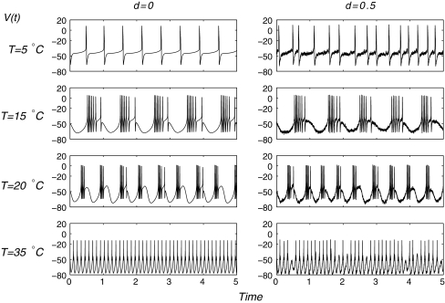
With temperature scaling and addition of noise, the cold receptors model (1)–(12) exhibits a broad range of different types of impulse patterns (Fig. 1). Also, the interval distributions of purely deterministic simulations (d = 0) exhibit considerable differences compared to the stochastic simulations. In the deterministic simulations we can see regular firing at low temperatures (at T = 5°C). For slightly higher temperature (T = 15°C) the firing pattern changers to burst discharges. The bursts become continually shorter if we increase the temperature further (up to T = 20°C). Simultaneously, the number of spikes per burst is reduced. For high temperatures again regular single-spike activity of increasing frequency occurs (T = 20°C).

Fig. 1.

Comparison of deterministic (d = 0) and stochastic (d = 0.5) simulations at different temperatures T (indicated on the left) of the model

In the stochastic simulation (d = 0.5), some fluctuations of spike-timing are visible. The patterns qualitatively change where bursts are occasionally skipped (for example at T = 35°C). At 35°C, instead of regular single-spike generation, some of the oscillations trigger spike doublets (two spikes per oscillation cycle). Initially, the two interval-bands of burst discharges (short intraburst intervals and longer burstpauses) are clearly separated from the interval-band of ongoing single- spike discharges. Noise also can prevent spike-generation in a deterministically regular spiking situation as it is shown (35°C), although with only several skipping.

Comparison of noisy and deterministic bifurcation diagrams

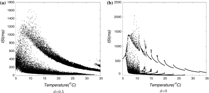
We use bifurcation diagrams to show major differences between noisy and deterministic simulations, in which successive interspike-intervals are plotted versus time as a function of temperature scaling. This computer model exhibits temperature dependencies in noisy simulations (Fig. 2a) that fairly well mimic the main characteristics of the experimental cold-receptor data. For comparison, a deterministic simulation is shown in Fig. 2b which shows abrupt transitions between different dynamical states. In the more realistic noisy simulation, there are distinct potential oscillations which generate regular burst discharges at mid-temperatures. At higher temperatures, the oscillations are accelerated which reduces the number of spikes per burst until the pattern changes to single-spike activity. In this situation, noise plays an essential role: spike generation is clearly phase-locked to the underlying oscillations, but noise determines the threshold crossings.

Fig. 2.

Bifurcation plots with respect to variation of the temperature. a Noisy simulations and b Deterministic simulations

Noisy simulations reflect more realistically experimental data, we used deterministic simulations (Fig. 2b) to show properties of dynamics that might be concealed in the noisy simulations. Starting from high temperatures, the behavior of the model changes form subthreshold oscillations to regular single-spike. Towards lower temperatures, there are several abrupt transitions from period-one to period-four whenever the number of spikes per oscillation cycle increases. At a certain temperature (15°C), a increasing number of bifurcations occurs followed by chaotic patterns. At still lower temperature (below about 7°C) the chaotic dynamics again disappear and are replaced by regular single-spike activity.

Altogether, at mid-temperatures, the abrupt transitions of deterministic simulation are completely smoothed out with noise which can be seen in the interval plot. The qualitative differences occur in the lower and upper extremes of the temperature range with the appearance of skipping in the noisy simulations and the transitions to chaotic interval sequences in deterministic simulations.

The return plots of deterministic and stochastic spike trains at different temperatures

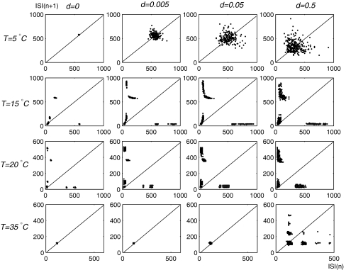
Another way to highlights the qualitative differences between the deterministic and noisy simulations is return plots of inter-spike intervals, plotting ISI (n + 1) versus ISI(n). Figure 3 shows return plots from simulation runs at the four different temperatures considered in this paper (top to bottom) and for four different levels of noise intensity (left to right).

Fig. 3.

Return plots from simulation runs at temperatures T = 5, 15, 20, and 35°C (top to bottom) and noise levels d = 0, d = 0.005, d = 0.05, d = 0.5 (left to right)

The top row and the bottom row of Fig. 3 show the tonic firing regimes at T = 5°C and T = 35°C. In the deterministic case (d = 0) there is only one tight cluster of dots around the fixed point on the 45° line which reflects regular tonic firing. For T = 5°C (top row), the cluster broadens strongly with increasing noise intensity d. Especially, the return plot at d = 0.5 shows no longer a circular distribution of points but spreads across a much larger area. At T = 35°C, the effect of noise is less pronounced for low noise levels (up to d = 0.005). More remarkable is the elongation of the clusters along the abscissa and ordinate with the increasing of the noise intensity (d = 0.5), this can be ascribed to increasing variability of spike-timeing due to the skipped spikes.

Row 2 and 3 of Fig. 3 show the bursting regimes at T = 15°C and T = 20°C. The additional clusters include long-short and short-long interval pairs, indicating the occurrence of skippings and intervals between bursts, as well as very short intervals, indicating burst discharges.

In the each return plot the left upper cluster indicates that longer burst-pauses are followed by short intraburst-intervals and the right lower cluster reflects the end of the bursts where short intraburst-intervals are followed by longer burst-pauses. A third cluster of short-short intervals is built up from the intraburst sequences.

The ISI-distance of deterministic and stochastic spike trains at different temperatures

In this section, we study the effect of increasing noise intensity d on spike trains by measuring the distance between deterministic and noisy impulse patterns in model (1)–(11). This approach is based on the time intervals between successive spikes instead of the spike as the basic element for measuring the (dis)-similarity of two spike trains. Due to the self-adaptation of this measure, it lends itself naturally to the characterization of neuronal spike trains, which have typically well-defined spikes but involve a wide range of time scales.

Spike detection

The first ingredient necessary for computation of the ISI-distance is the extraction of the spike times by a spike detection algorithm. This transforms the continuous time series into a discrete series of binary (0–1) spikes. Here, we use the following spike detection algorithm: each spike train is expressed as a series of δ functions with t₁, …, t_M denoting the series of spike times and M being the number of spikes. In this study, the threshold is chosen as the maximum value of the action potential.

12

The ISI-distance

The distance between two spike trains is defined by the following procedure: in a first step the value of the current interspike interval at each time instant by

13

where are the spike times of the spike train x(t) as given by (12). In the same manner we obtain the function y_isi using the spike times . In the second step we take the normalized difference between two interspike intervals x_isi and y_isi as:

14

The value of I(t) becomes zero if the frequencies of two spike trains are same, and approach −1 and 1, respectively, if the firing rate of one spike train is much higher than the other spike train (Kreuz et al. 2007). Finally, the distance of spike train is computed using two possible averages. The time-weighted distance D_I is integrated over time:

15

The ISI-distance between the deterministic and stochastic spike trains

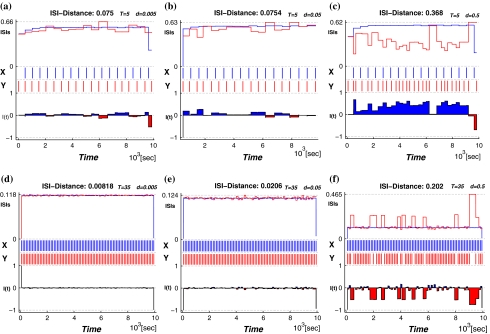
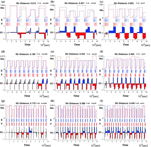
Then we use the ISI-distance (Kreuz et al. 2007) to characterize the distances between the deterministic and noisy spike trains. The subfigures of Fig. 4 have the structure as following: the middle row shows the two recorded time series where the spike train x is deterministic data (marked in blue) and y is a stochastic spike train with varying noise level (marked in red). The ISI-values according to Eq. 13 are shown in each top row, and the corresponding normalized ISI-distance (Eq. 14) are shown in the bottom row. The colors in the bottom row mark the times when the respective spike train is slower. The value of the ISI-distance sum appears as a label in the title of each subfigure.

Fig. 4.

The ISI-distance between the deterministic and stochastic spike trains for the period-one firing patterns. The temperature T is 5°C in the top row, and 35°C in the bottom row. The noise levels from left to right

Figure 4 presents the firing regimes at T = 5°C and T = 35°C. The spike train x(t) is the deterministic data. When we add noise we observe fluctuations in the spike-timing of spike train y(t). Each sub-figure from left to right shows the distance between the deterministic spike train and the stochastic one at varying levels of the noise intensity. The data for the spike train x is identical in each row of subfigures:(a)–(c) and (d)–(f), respectively. As the noise density increases from d = 0.005 to d = 0.5 in each row the fluctuations of the spike times in y(t) become stronger.

The ISI-distances are also consistently larger for each noise level at high temperature(T = 35°C) than at low temperature(T = 5°C) due to the high frequency of spike firing. The fluctuations are smaller even relative to the shorter interspike times in the train for high temperature.

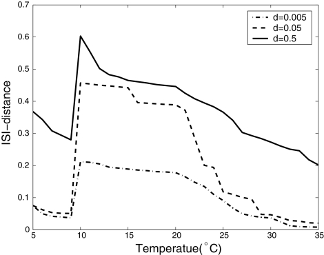
Figure 5 shows the ISI-distances for the bursting regimes between the deterministic spike trains and the noisy ones(T = 10, 15, and 20°C). Similarly to the period-one firing in Fig. 4, at each fixed temperature, the ISI-distance increases with the noise intensity becoming larger(see each horizontal row of the figure from left to right). For example, at T = 10°C, with the d changing from 0.005 to 0.5, the ISI-distance changes from 0.212, 0.457 and 0.603, which means that the higher noise intensity causes stronger fluctuations of the times between spikes in the spike train. While for each fixed noise level and increasing temperature(see each vertical column of Fig. 5 from top to bottom), the number of spikes in each burst decreases and the ISI-distance to the deterministic spike train also decreases. In Fig. 6, we give the the change in the ISI-distance as a continuous function of temperature at three different noise intensity.

Fig. 5.

The ISI-distance for the bursting regimes. The temperature T in the top row is 10°C, in the middle rowT is 15°C, and in the bottom rowT is 20°C. The noise intensity increases form left to right

Fig. 6.

The change of ISI-distance as continuous function of temperature

Conclusion

In conclusion, we study the noise effect in the temperature encoding of neuronal spike trains in a cold receptor model. With the addition of noise, this minimal model can generate a variety of impulse patterns and allow continuous transitions from rhythmic bursting to subthreshold oscillations with occasional spikes. Thus, noise can be seen as estimations of the actual dynamics underlying the experimental data. For example, the return plots indicate that longer intervals have a less exact phase-locking than shorter ones and suggest that noise is not only essential for spike-generation but also interferes with the oscillatory activity. This stochastic phenomena means that signal encoding can be different with the change of noise level. The result might also suitable for signal encoding in many other neurons in the peripheral and central nervous system in the mammalian brain. For a better understanding of noise effect, here, we use the ISI-distance to explore how noise affects the pattern variability of the cold receptor. The method and results in this study may be instructive for the study of neural encoding of spike trains under noisy environment. In our future study, we will consider the relationship between the effect of noise on ISI-distance and the dynamics of the firing patterns.

References

- Braun HA, Huber MT, Dewald M, Schäfer K, Voigt K. Computer simulations of neuronal signal transduction: the role of nonlinear dynamics and noise. Int J Bifurcat Chaos. 1998;8:881–889. doi: 10.1142/S0218127498000681. [DOI] [Google Scholar]
- Braun HA, Schäfer K, Voigt K, Peters R, Bretschneider F, Pei X, Wilkens L, Moss F. Low dimensional dynamics in sensory biology I: thermally sensitive electroreceptors of the catfish. J Comput Neurosci. 1998;4:335–347. doi: 10.1023/A:1008852000496. [DOI] [PubMed] [Google Scholar]
- Braun HA, Huber MT, Anthes N, Voigt K, Neiman A, Pei X, Moss F. Noise-induced impulse pattern modifications at different dynamical period-one situations in a computer model of temperature encoding. Biosystems. 2001;62:99–112. doi: 10.1016/S0303-2647(01)00140-X. [DOI] [PubMed] [Google Scholar]
- Braun HA, Voigt K, Huber MT. Oscillations, resonances and noise: basis of flexible neuronal pattern generation. Biosystems. 2003;71:39–50. doi: 10.1016/S0303-2647(03)00108-4. [DOI] [PubMed] [Google Scholar]
- Berry MJ, Warland DK, Meister M. The structure and precision of retinal spike trains. Proc Natl Acad Sci USA. 1997;94:5411–5416. doi: 10.1073/pnas.94.10.5411. [DOI] [PMC free article] [PubMed] [Google Scholar]
- Eiesinga TPH, Fellous JM, Sejnowski TJ. Attractor reliability reveals deterministic structure in neuronal spike trains. Neural Comput. 2002;14:1629–1650. doi: 10.1162/08997660260028647. [DOI] [PubMed] [Google Scholar]
- Fox RF, Gatland IR, Roy R, Vemuri G. Fast, accurate algorithm for numerical simulation of exponentially correlated colored noise. Phys Rev A. 1998;38:5938–5940. doi: 10.1103/PhysRevA.38.5938. [DOI] [PubMed] [Google Scholar]
- Gutfreund Y, Yarom Y, Segev I. Subthreshold oscillations and resonant frequencies in guinea-pig cortical neurons, physiology and modelling. J Physiol. 1995;483:621–640. doi: 10.1113/jphysiol.1995.sp020611. [DOI] [PMC free article] [PubMed] [Google Scholar]
- Horsthemke W, Lefever R. Noise-induced transitions. Berlin: Springer; 1984. [Google Scholar]
- Hodgkin AL, Huxley AF. A qualitative description of membrane current and its application to conduction and excitation in nerve. J Physiol. 1952;117:500–544. doi: 10.1113/jphysiol.1952.sp004764. [DOI] [PMC free article] [PubMed] [Google Scholar]
- Hunter JD, Milton G. Amplitude and frequency dependence of spike timing: implications for dynamic regulation. J Comput Neurosci. 2003;90:387–394. doi: 10.1152/jn.00074.2003. [DOI] [PubMed] [Google Scholar]
- Kreuz T, Haas JS, Morelli A, Abarbanel HDI, Politi A. Measuring spike train synchrony. J Neurosci Meth. 2007;165:151–161. doi: 10.1016/j.jneumeth.2007.05.031. [DOI] [PubMed] [Google Scholar]
- Lindner B, Garciaa Ojalvo J, Neiman A, Schimansky-Geier L. Effects of noise in excitable systems. Phys Rep. 2004;392:321–424. doi: 10.1016/j.physrep.2003.10.015. [DOI] [Google Scholar]
- Mainen Z, Sejnowski TJ. Reliability of spike timing in neocortical neurons. Science. 1995;268:1503–1506. doi: 10.1126/science.7770778. [DOI] [PubMed] [Google Scholar]
- Pare D, Pape HC, Dong J. Bursting and oscillating neurons of the cat basolateral amygdaloid complex in vivo, electrophysiological properties and morphological features. J Neurophysiol. 1995;74:1179–1191. doi: 10.1152/jn.1995.74.3.1179. [DOI] [PubMed] [Google Scholar]
- Quian Quiroga R, Kreuz T, Grassberger P. Event synchronization: a simple and fast method to measure synchronicity and time delay patterns. Phys Rev E. 2002;66:041904. doi: 10.1103/PhysRevE.66.041904. [DOI] [PubMed] [Google Scholar]
- Schreiber S, Fellous JM, Whitmer JH, Tiesinga PHE, Sejnowski TJ. A new correlation-based measure of spike timing reliability. Neurocomputing. 2003;52:925–931. doi: 10.1016/S0925-2312(02)00838-X. [DOI] [PMC free article] [PubMed] [Google Scholar]
- Victor JD, Purpura K. Nature and precision of temporal coding in visual cortex: a metric-space analysis. J Neurophysiol. 1996;76:1310–1326. doi: 10.1152/jn.1996.76.2.1310. [DOI] [PubMed] [Google Scholar]
- Rossum MCW. A novel spike distance. Neural Comput. 2001;13:751–763. doi: 10.1162/089976601300014321. [DOI] [PubMed] [Google Scholar]
- Singer Wolf. Distributed processing and temporal codes in neuronal networks. Cogn Neurodyn. 2009;3:189–196. doi: 10.1007/s11571-009-9087-z. [DOI] [PMC free article] [PubMed] [Google Scholar]
- Walter JF. Deep analysis of perception through dynamic structures that emerge in cortical activity from self-regulated noise. Cogn Neurodyn. 2009;3:105–116. doi: 10.1007/s11571-009-9075-3. [DOI] [PMC free article] [PubMed] [Google Scholar]