Improved Dynamic Cardiac Phantom Based on 4D NURBS and Tagged MRI

Abstract

We previously developed a realistic phantom for the cardiac motion for use in medical imaging research. The phantom was based upon a gated magnetic resonance imaging (MRI) cardiac study and using 4D non-uniform rational b-splines (NURBS). Using the gated MRI study as the basis for the cardiac model had its limitations. From the MRI images, the change in the size and geometry of the heart structures could be obtained, but without markers to track the movement of points on or within the myocardium, no explicit time correspondence could be established for the structures. Also, only the inner and outer surfaces of the myocardium could be modeled. We enhance this phantom of the beating heart using 4D tagged MRI data. We utilize NURBS surfaces to analyze the full 3D motion of the heart from the tagged data. From this analysis, time-dependent 3D NURBS surfaces were created for the right (RV) and left ventricles (LV). Models for the atria were developed separately since the tagged data only covered the ventricles. A 4D NURBS surface was fit to the 3D surfaces of the heart creating time-continuous 4D NURBS models. Multiple 4D surfaces were created for the left ventricle (LV) spanning its entire volume. The multiple surfaces for the LV were spline-interpolated about an additional dimension, thickness, creating a 4D NURBS solid model for the LV with the ability to represent the motion of any point within the volume of the LV myocardium at any time during the cardiac cycle. Our analysis of the tagged data was found to produce accurate models for the RV and LV at each time frame. In a comparison with segmented structures from the tagged dataset, LV and RV surface predictions were found to vary by a maximum of 1.5 mm’s and 3.4 mm’s respectively. The errors can be attributed to the tag spacing in the data (7.97 mm’s). The new cardiac model was incorporated into the 4D NURBS-based Cardiac-Torso (NCAT) phantom widely used in imaging research. With its enhanced abilities, the model will provide a useful tool in the study of cardiac imaging and the effects of cardiac motion in medical images.

I. Introduction

Simulation is a powerful tool for characterizing, evaluating, and optimizing medical imaging systems. An important aspect of simulation is to have a realistic phantom or model of the human anatomy from which to evaluate imaging procedures and techniques. Previously, we developed a realistic phantom for the cardiac motion for use in medical imaging research [1]. The phantom was based on a gated magnetic resonance imaging (MRI) cardiac study of a normal patient using non-uniform rational b-spline (NURBS) surfaces to model the different structures of the heart. 3D NURBS surface models for the principal parts of the heart, the right and left ventricles, atria and the outer surface of the heart, over the cardiac cycle were developed. These surfaces were then spline-interpolated about a fourth dimension, time, creating a set of 4D NURBS surfaces or a set of 3D NURBS surfaces changing in time. This 4D heart model was incorporated into the 4D NURBS-based Cardiac-Torso (NCAT) phantom [2] (Fig. 1), a computerized model of the human body that is widely used in medical imaging research.

Fig. 1.

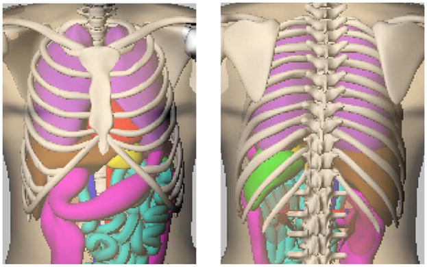
Anterior (left) and posterior (right) views of the 4D NCAT phantom.

The initial 4D cardiac model provided an accurate representation of the change in size and geometry of the heart structures during the cardiac cycle, but without markers to track points on or within the myocardium, no explicit time correspondence could be established for the structures. In addition, the internal motion of the heart was not represented since only the inner and outer surfaces of the heart were modeled. In this work, we seek to enhance this model of the beating heart using 4D tagged MRI data.

Tagged MRI [3]–[9] consists of a series of magnetic resonance images with tags defined as spatially encoded magnetic saturation pulses. The tags, which appear as dark bands in the MRI images, can be arranged in different patterns including parallel lines, a grid, or radial stripes. The tags move with the underlying tissue allowing the tracking of its motion in a time series of MR images.

Using MRI tagging to analyze cardiac motion involves three steps. First, a tagging pattern is placed in the myocardial tissue with spatially selective rf pulses. Generally, tags are arranged as sets of parallel lines due to the speed with which they may be generated and subsequently imaged [10]. A sequence of MR images is then obtained in which the motion of the tagging pattern can be observed. The changes of the tagging pattern among the time-sequence MR images are then used to solve for the motion of the myocardium. The deformation of parallel tagging planes provides only one-dimensional motion information of the myocardium. In order to analyze the entire 3D motion of the heart, three independent tagging directions (x, y, and z) must be analyzed and combined.

Several methods have been used to analyze the motion of the heart from tagged MRI images based on that of the tag lines [11]. In our work to create an improved cardiac phantom, we utilize a similar method to that of Ozturk et al. [12] to analyze the heart motion from three sets of tagged MR images, two sets of short-axis slices and one set of long-axis slices. In this method, 2D b-spline displacement fields (or surfaces) are fit to each image plane in two short-axis image sets (the same anatomical slices in each set but with the tag lines arranged orthogonally so as to follow the x- and y-deformations of the heart) and one long-axis image set to follow the z-deformation. The 2D b-spline displacement fields are used to interpolate the motion of points anywhere within the image planes. At each time point in the cardiac cycle, spline interpolation is performed between the image planes forming a 3D b-spline displacement field for the image volume for each image set. Spline interpolation is then performed over time to form a 4D displacement field for each of the three image sets. The three 4D displacement fields can be used to track the 3D deformation of points anywhere within the image volume and more specifically the myocardium.

In our implementation of the above method, we use NURBS surfaces to calculate the displacement fields. NURBS can model complicated shapes and objects more accurately than regular b-splines. Using this NURBS-based analysis, we created an enhanced computer model for the beating heart with a realistic time correspondence defined for the cardiac structures based on tagged MRI data. The heart model was incorporated into the 4D NCAT phantom where it will provide a vital tool to research existing and emerging imaging techniques used in the diagnosis of cardiac disease.

II. Methods

A. Tagged MRI Data

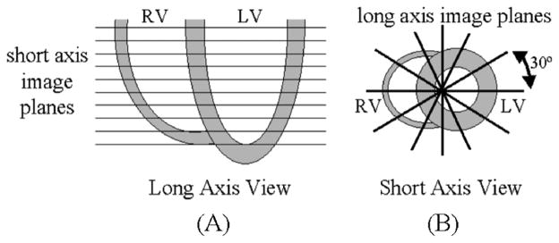
Three sets of electrocardiogram (ECG)-gated tagged MR images from a normal subject were used to analyze the heart motion. The datasets were obtained from Drs. Elliot McVeigh, Cengiz Ozturk, and Daniel Ennis from the Johns Hopkins University. They were acquired in a similar manner to those used in the study by Ozturk et al. [12]. The sets of data spanned the left ventricle and were acquired for 26 time frames over the cardiac cycle. The data included two sets of short-axis (SA) images and one set of long-axis (LA) images. The SA image sets consist of stacks often 256 × 256 SA images from base to apex as seen in Fig. 2(a). The pixel width and slice thickness of the SA images was 1.328 mm and 6.98 mm respectively for both sets of data. The parallel tag lines (width = 2 pixels or 2.656 mm’s) in the two SA image volumes were orthogonal with respect to one another to analyze the x- and y- deformations of the heart. The LA images were radially oriented and spaced every 30° (Fig. 2(b)). The pixel width of the LA images was also 1.328 mm. The tag lines in the LA image volume were designed to be parallel to the SA image planes to analyze the z-deformation of the heart.

Fig. 2.

Acquired image planes for the tagged MRI data. (A) The two sets of short-axis images were acquired on 10 image planes spanning the left ventricle. (B) The 6 long-axis images were acquired on radially oriented image planes spaced 30 degrees apart.

Each image slice in a set of tagged data was collected separately over an average beating heart cycle. During the acquisition of images, the subject was instructed to hold their breath so that the respiratory motion would not interfere in the acquisition process. The tagging planes were initialized at end-diastole (ED) and 26 time frames were obtained over the cardiac cycle with breath holding. Fig. 3 shows example images from the three sets of tagged MRI data, the two short-axis sets (SA1 and SA2) and the long-axis set (LA1). The tagging pattern in each image slice starts as a set of parallel stripes. As the heart moves, the stripes deform with the movement of the underlying myocardium. The deformation of the tags can be used to analyze the motion of the heart tissue in the direction perpendicular to that of the tag lines. The two SA image sets are used to analyze the x- and y- deformation of the heart tissue. The LA image set is used to analyze the z-deformation.

Fig. 3.

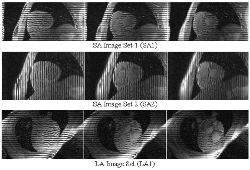
Tagged MR Data. The data consists of two sets of orthogonal SA images and one set of LA images. For each set, one image is shown at three different time frames for one half of the cardiac cycle from end-diastole (left) to end-systole (right). For each slice, the tag lines begin as parallel stripes then deform with the movement of the underlying heart tissue.

The sets of tagged images were analyzed using FindTags [13], a software application developed at Johns Hopkins University. The FindTags program was used to determine the endo- and epicardial borders of the LV as seen in Fig. 4(a). FindTags was not used to determine the endo- and epicardial borders of the RV. This was done using another program as will be discussed later. After determining the contours of the LV, the tag lines for each image were segmented (Fig. 4(b)). The 676 tag images comprising the three sets of tagged data were each analyzed using the FindTags program. The contour and tag line information from each image was saved in a file containing points (spaced every pixel) defining the contours and tag lines in that image. The output file for each image also contained a coordinate system transform that would transform the points in 2D image coordinates into a fixed 3D laboratory coordinate system.

Fig. 4.

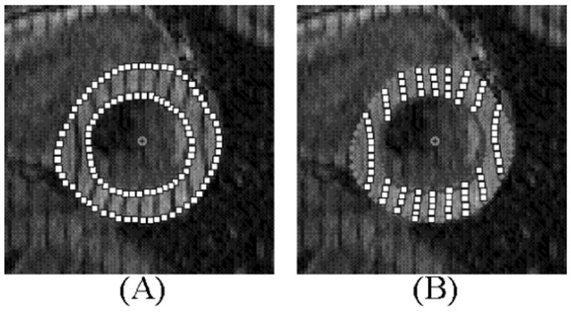
Analysis of tagged images using the FindTags program. (A) Endo- and epicardial borders of the LV are segmented using the semi-automatic algorithm. (B) Tag lines are then segmented automatically. The points defining the contours and tag lines can be saved to an output file. The spacing and size of the points in the above figure were done for illustration. In Findtags, the points are the size of one pixel and are spaced every pixel.

B. Alignment of the Tagged Data

Breath holding was used to minimize the effects of respiratory motion on the tagged data. However, the point during the respiratory cycle at which the subject held their breath might not be exactly the same for each set of image data. As a result, misalignment was found to occur between the two orthogonal sets of short-axis tagged data and between the short-axis and the long-axis data due to different breath holding positions. From the examination of the images, the respiratory motion of the heart was found to mainly involve a simple global translation. Alignment between the sets of images was checked for the initial time frame for each acquisition period. The alignment was checked through a comparison of the epi- and endocardial LV contours found for each image slice.

Once the data was aligned correctly, 2D NURBS displacement fields or surfaces were fit to the realigned tag lines as will be discussed in the following section.

C. Development of the 2D NURBS Tagging Plane

We developed a 2D NURBS field or surface in order to follow the tag lines in each image slice. A NURBS surface (Fig. 5) is a bidirectional parametric representation of an object. Points on a NURBS surface are defined by two parametric variables, u (0 ≤ u ≤ 1) and v (0 ≤ v ≤ 1), usually representing longitude and latitude respectively. Points defined in Cartesian coordinates (x, y, z) can easily be converted into surface coordinates (u and v) and vice versa. A 2D NURBS surface of degree p in the u direction and degree q in the v direction is defined as a piecewise ratio of b-spline polynomials as given by the following function [14], [15]

Fig. 5.

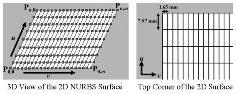
2D NURBS surface developed to follow the tag lines of the image planes. The knots (solid lines) of the surface were setup to form a 2D grid. Knot lines running in the v direction were spaced with the tag spacing of the images which was 7.97 mm. The knot lines running in the u direction were spaced more frequently at 1.65 mm for increased sampling. For our work, the 2D NURBS surface was defined with n = 23 and m = 103. The control points and grid points (squares) of the initial surface are located at the intersection of the knot lines.

$$\mathbf{S}(u,v)=\frac{{\displaystyle \sum _{i=0}^n}{\displaystyle \sum _{j=0}^m}{N}_{i,p}(u)N_{j,q}(v){\mathbf{P}}_{i,j}}{{\displaystyle \sum _{i=0}^n}{\displaystyle \sum _{j=0}^m}{N}_{i,p}(u)N_{j,q}(v)}$$ (1)

where S is a point on the surface defined in Cartesian coordinates (x, y, z), n and m are the number of control points in the u and v directions respectively, P_i,j is the n × m matrix of control points also defined in Cartesian coordinates, and N_i,P(u) and N_j,_q(v) are polynomial functions of degree p and q respectively.

The coordinates of S are determined by a function of the parameters u and v. The function consists of a weighted sum of the n × m matrix of control points P_i,j. The weighting factors are the polynomial functions N_i,p(u) and N_j,q(v). The polynomial functions N_i,p(u) and N_j,q(v) are the b-spline basis functions defined on the knot vectors U and V defined by the following equations

$$\mathbf{U}=\left(\underset{p=1}{\underbrace{0,\dots ,0}},u_{p+1},\dots ,u_{r-p-1},\underset{p+1}{\underbrace{1,\dots ,1}}\right)$$ (2)

$$\mathbf{V}=\left(\underset{q=1}{\underbrace{0,\dots ,0}},u_{q+1},\dots ,u_{s-q-1},\underset{q+1}{\underbrace{1,\dots ,1}}\right)$$ (3)

where r = n + p + 1 and s = m + q + 1. The knot vectors define lines which divide the surface into different segments. Each segment of the surface has its own distinct set of polynomial functions which help to define the shape of the segment.

The 2D NURBS surface for the displacement fields was defined as a cubic surface (p = q = 3) and was set up so that its knot lines formed a 2D Cartesian coordinate system (Fig. 5). The horizontal knots traveling in the v direction of the surface were spaced vertically every 7.97 mm according to the spacing of the tag lines in the tagged images. The vertical knots traveling in the u direction of the surface were spaced horizontally to sample the 2D plane every 1.65 mm. The surface was composed of a 103 × 23 set of control points. The control points of the surface were located at the intersection of the knot lines.

D. Fitting of the 2D NURBS Surfaces to the Image Planes

As mentioned earlier, the tag lines in the tagged images were initialized at the end-diastolic time frame (frame 1). The tag lines were formed based on the tag points found through the FindTags program (Fig. 4). At frame 1, the tag lines start as sets of parallel lines. For each image plane at time frame 1 in a set of tagged images, a 2D NURBS surface was placed so that the knots in the v direction were directly over the tag lines (formed from the tag points) as seen at the left of Fig. 6. This associated each tag line, Ti, in the image with a knot, v_i, on the 2D surface. This initial surface was set as the base surface from which following time frames were analyzed. For each subsequent time frame, the base surface for each image plane was deformed so that each knot, v_i, would match its corresponding tag line, T_i, located in that image plane as shown at the right of Fig. 6. The surface was deformed by translating the control points located along the path of the knot in the direction perpendicular to this path. The following describes the method used to manipulate the control points of the 2D NURBS surface to match the tag lines on an image plane.

Fig. 6.

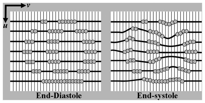
Fitting of the 2D NURBS surface to the tagged images. For each image plane in a set of tagged images, the knots of a 2D NURBS surface are aligned with the tag lines (dark lines in the figure) formed from the tag points (grey circles) at ED (frame 1). This surface serves as the base surface from which subsequent time frames will be analyzed. For each subsequent frame, the control points along the knots in the v direction of the base surface are manipulated so that the knots of the surface match the tag lines.

An automatic algorithm was developed to manipulate the control points of the initial 2D NURBS surface defined for an image plane so that each knot, v_i, of the surface matched its corresponding tag line, T_i, located in the image plane. This algorithm was used to match the knots of the surface to the tag lines of the image plane at each time frame in the cardiac cycle. By doing this, the knots of the surface deform with the tag lines defined for the image plane. The algorithm started with the output file obtained from the FindTags program for a particular image. Contained in the file were points defining the individual tag lines in the image. Using the points for each tag line, the program first fit a cubic NURBS curve to these points using accepted methods for fitting a cubic NURBS curve to a set of points [14], [15].

The 2D NURBS surface S(u, v) is defined by (1). The piece-wise rational basis functions R_i,j of the NURBS surface are defined in (4). These functions help to form the shape of the surface by weighting the surface’s control points P_i,j.

$$R_{i,j}(u,v)=\frac{N_{i,p}(u)N_{j,q}(v)}{{\displaystyle \sum _{i=0}^n}{\displaystyle \sum _{j=0}^m}{N}_{i,p}(u)N_{j,q}(v)}.$$ (4)

With this definition, the NURBS surface equation can be rewritten as

$$\mathbf{S}(u,v)=\sum _{i=0}^n\sum _{j=0}^m{R}_{i,j}(u,v){\mathbf{P}}_{i,j}.$$ (5)

The surface contains many grid points P_grid, which are defined as a point on the surface at which the orthogonal knots intersect. Initially at time frame 1, these points are at the same location as the surface’s control points, which control the shape of the surface. Each grid point is defined in terms of the parametric variables (u and v) of the surface as shown by (6).

$${\mathbf{P}}_{\mathit{grid}}=\mathbf{S}(\overline{u},\overline{v}).$$ (6)

For each tag line Ti, the grid points on the surface located on the knot v_i have to be manipulated in order to fit the tag line. Each grid point on the knot v_i must be moved to a new point P̂_grid located on the NURBS curve for the tag line T_i. In order to find the new location for the grid point, the NURBS curve for that tag line was intersected with the u knot of the grid point as shown in Fig. 7. The intersection point was found by a bisection routine [16]. Points on the curve were successively sampled in halves until the intersection point was found within a predetermined tolerance value (0.001).

Fig. 7.

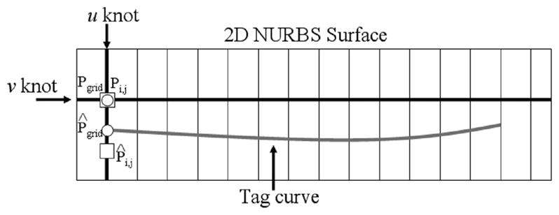
Fitting of a v knot line of the 2D NURBS surface to a tag line. A NURBS curve (grey) approximates the tag line. Each grid point along the knot line needs to be repositioned to corresponding points on the NURBS curve. The new position for each grid point is found by intersecting the NURBS curve with the u knot of the grid point. For example, the grid point P_grid (circle) needs to be moved to the new location P̂_grid on the tag curve. The grid point is moved by altering the location of the corresponding surface control point P_i,j (square). The control point is initially located at the same location of the grid point (intersection of the knots). Movement of the control point does not correspond one to one with the movement of the grid point, however. In the above example, the control point P_i,j must be moved a greater distance in order to set the grid point in the desired location. Control points are manipulated in this manner for all grid points of the v knot line to fit it to the tag curve.

Once the desired location for the grid point was found on the tag line curve, the change in position, V, of the grid point was calculated by (7).

$$\mathbf{V}={\widehat{\mathbf{P}}}_{\mathit{grid}}-{\mathbf{P}}_{\mathit{grid}}.$$ (7)

The displacement P_disp for the point was calculated as the total distance between the original and desired locations of the grid point by the following equation.

$$P_{\mathit{disp}}=\mid \mathbf{V}\mid .$$ (8)

An average displacement for the tag line, T_disp, was computed by averaging the displacement for each of the N grid points defining the tag line as shown in (9).

$$T_{\mathit{disp}}=\frac{{\displaystyle \sum _{i=1}^N}{P}_{{\mathit{disp}}_i}}{N}.$$ (9)

The average displacement T_disp for each of the M tag lines was then averaged into one final displacement value I_disp for the image plane.

$$I_{\mathit{disp}}=\frac{{\displaystyle \sum _{i=1}^M}{T}_{{\mathit{disp}}_i}}{M}.$$ (10)

The control point P_i,j, defined for the grid point was then translated until the grid point was moved to the desired location. Movement of the control point does not correspond one to one with the movement of the grid point. Control points are points that define the shape of the surface, but they are not necessarily points on the surface. The amount α with which the control point was translated was determined by the following equation.

$${\alpha }_{i,j}=\frac{P_{\mathit{disp}}}{R_{i,j}(\overline{u},\overline{v})}.$$ (11)

The new location of the control point P^_i,j was calculated according to (12).

$${\widehat{\mathbf{P}}}_{i,j}={\mathbf{P}}_{i,j}+{\alpha }_{i,j}\mathbf{V}.$$ (12)

The grid points were manipulated in this manner until the total displacement for the image I_disp was less than a set tolerance value (0.001). Two hundred and sixty 2D NURBS surfaces were fit to each set of short-axis images (10 image planes × 26 time frames). The 2D NURBS surface of Fig. 6 was rotated 90 degrees so as to fit the orthogonal tag lines of the short-axis set of SA2. One hundred and fifty-six 2D surfaces were fit to the set of long-axis images (6 image planes × 26 time frames).

Once the 2D surfaces were fit to the image planes, the surfaces were transformed into the 3D laboratory coordinate system using the transforms found in the FindTags files. The surfaces were then used as fields to track the x-, y-, and z-deformations of the heart. The motion analysis performed using these surface fields was used to build 4D models for the left and right ventricles. The following section discusses the generation of these models.

E. Creation of the LV and RV Models

The SURFdriver program [17], a surface reconstruction application, was used to create initial polygon models for the LV and RV. The program was used to display one set of tagged short-axis images for the end-diastolic time frame. Points defining the contours of the inner and outer walls of the LV were input into SURFdriver from the output files from the FindTags program. FindTags was not used to segment the RV as it was for the LV; therefore, the inner and outer contours of the RV were determined manually using the SURFdriver program. The contours for each surface of the LV and RV at ED were lofted into 3D cubic NURBS surfaces using standard techniques for generating smooth cubic NURBS surfaces from the contours of an object [14], [15]. As can be seen in Fig. 8, the short-axis images did not span the entire length of the ventricles. The top (base) of the ventricles and the bottom (apex) are not fully covered by the SA image slices. These regions will be approximated using the LA image slices as discussed later.

Fig. 8.

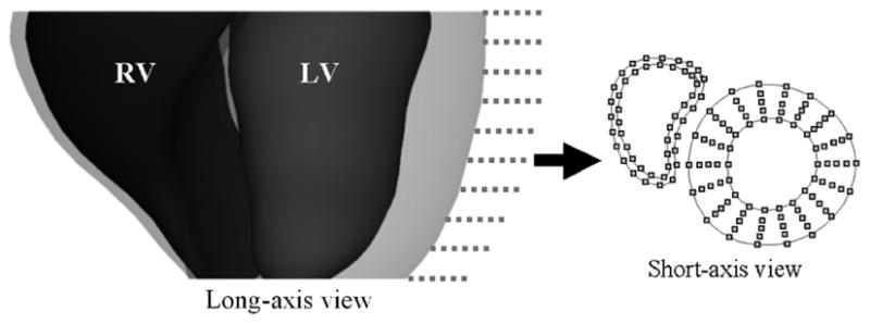
Points on the endo- and epicardial surfaces of the LV and RV at end-diastole sampled on the SA image planes (dotted lines). Linear interpolation is performed between the points on the endo- and epicardial borders of the LV to obtain points for three mid-ventricular surfaces. One example short-axis slice is shown with the sampled points for the five LV surfaces and the two RV surfaces. The LV and RV are separated by a space in the short-axis slice to distinguish the points for each structure at the RV-LV junction.

To track the motion of the heart, points were sampled from each 3D NURBS surface for the RV and LV at ED on the planes defined by the SA images. For the endo- and epicardial surfaces defining the LV, 18 points were radially sampled for each of the ten SA image planes resulting in 180 points per surface as shown in Fig. 8. Three mid-ventricular contours were obtained for the left ventricle by linearly interpolating between the sampled points for the inner and outer contours. Linear interpolation was used so the points were equally distributed about the LV thickness. For each surface defining the RV, 24 points were sampled for each of the ten SA image planes (240 total points per surface). Due to the crescent shape of the RV, the points were not sampled radially as they were for the LV. This would result in an unequal sampling of points; therefore, the points were sampled in equal increments along the path of the RV contours.

The points defining each structure were then located on the 2D NURBS surface fields defined at ED for the short-axis image plane on which they were sampled (Fig. 9(a)). They were located twice for each slice, once in the NURBS surface defined for SA1 and again in the NURBS surface defined for SA2. The points were located by sampling the 2D NURBS surfaces in the u and v directions in small increments. Each sampled surface point S(ū, v̄) was compared to the point P that was being looked for, and the difference S_diff was calculated by the following equation

Fig. 9.

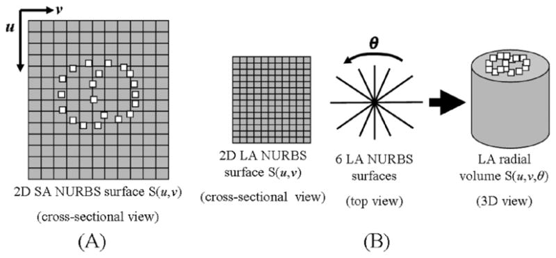
(A) Points defining the structures of the RV and LV were defined in surface coordinates (u, v) on the 2D NURBS surfaces for the SA image on which the points were sampled. The NURBS surface fields for the SA images are used to follow the x- and y-deformation of the points for subsequent time frames. (B) The six 2D NURBS surface fields for the LA images at end-diastole were splined about the radial direction θ to form a radial volume. The points defined for the LV and RV were located in volume coordinates (u, v, θ) of the radial volume at end-diastole. Image volumes were similarly created for subsequent time frames, and the volume coordinates were used to track the z-deformation of the points.

$$S_{\mathit{diff}}=\mid \mathbf{S}(\overline{u},\overline{v})-\mathbf{P}\mid .$$ (13)

Each point P was defined in surface coordinates by the combination (ū, v̄) that resulted in the smallest difference. Using the surface coordinates (u, v), the motion of the points can be tracked using the 2D NURBS surface fields defined for each time frame of the cardiac cycle. The surface points deform with the time series of 2D NURBS surfaces according to the motion of the tag lines. Using the two sets of short-axis surface fields can, therefore, follow the in plane (x, y) motion of the myocardium The short-axis set SA1 can track the x-coordinate for a point over time while the SA2 can track the y-coordinate.

To complete the analysis of the 3D motion, the long-axis surface fields must be used to follow the z-deformation or motion between planes. The six 2D NURBS surfaces of the LA image set defined at ED were spline-interpolated radially to form a 3D volume using the 4D NURBS technique developed previously [1] (Fig. 9(b)). The radial volume S(u, v, θ) is now defined by three parametric variables u, v, and θ, with θrepresenting the radial sampling. The (x, y, z) coordinates of the points for each surface were defined in volume coordinates (u, v, θ) of the new 3D radial volume using the technique described above for the SA image surfaces. However, in addition to stepping in the u and v directions, the additional radial direction θ is needed. Radial volumes were similarly created for subsequent time frames after ED, and the volume coordinates were used to track the z-deformation of the points defining the left and right ventricles.

As mentioned earlier, the SA image planes do not fully cover the LV and RV. The LA images were used to estimate the motion of the LV and RV at the base of the ventricles and at the apex. The six LA image slices defined at the end-diastolic time frame were examined visually locating the atrioventricular (AV) valve plane indicating the top (base) of the ventricles. The contours for the endo- and epicardial borders of the LV obtained using the FindTags program and those for the RV obtained using the SURFdriver program for the six slices were intersected with the AV plane producing points on this plane from the contours. These points on the long-axis image planes were tracked in subsequent time frames using the 2D NURBS surface fields for the individual LA image slices. The points were then used to create cubic NURBS curves for the borders of the LV and RV at the AV plane for each time frame. The LV contours defined at each time frame were sampled radially every 20 degrees to provide 18 points on this plane for the LV models. The RV contours were sampled in equal increments to provide 24 points on the AV plane for the RV models. Linear interpolation was used between the points defined for the inner and outer borders of the LV to get points for the mid-ventricular surfaces. The LA image slices were also examined for the apex of the RV and LV. The apex of the RV and LV was found for each of the 26 time frames by visually inspecting the tagged images. The location of the apex of the left and right ventricles was noted and stored with the other tracked points.

Using the short-axis and long-axis NURBS surface fields, the motion of the points for the LV and RV defined by the SA image planes was tracked over the 26 time frames. These were then used in combination with the points tracking the base and apex of the ventricles to form 3D NURBS surface models for LV and RV at each time frame in the cardiac cycle. The 3D surface models for the RV and LV were formed from initial template surfaces. The template surface for each structure serves as a placeholder to input tracked points from the tagged MRI analysis. Using the NURBS modeling software Rhinoceros [18], we built template half-ellipsoid models from which to input the tracked points for the LV and RV models. We created one half-ellipsoid for the LV consisting of 12 knots with 18 control points equally distributed radially along each knot. We created a similar ellipsoid for the RV consisting of 12 knots with 24 control points distributed equidistant along each knot. The control points for these surfaces were distributed in the same pattern as our tracked points. The half-ellipsoid developed for the LV is shown in Fig. 10. For each time frame, the control points of the half-ellipsoids, which lie approximately on the surface, were determined by the tracked points for each model. The control points of the middle ten knots were set according to the tracked points located on the ten short-axis image planes. The control points of the uppermost knot were set according to the tracked points defining the antrioventricular (AV) plane. The points for the bottom knot were set to the point defining the apex in the long-axis slices. Each LV and RV surface for each of the 26 time frames was created by using the tracked points to set the surface’s control points. The control points define the shape of a NURBS surface. Setting them to match the tracked points alters the shape of the half ellipsoid to match that of the particular heart structure. By using the same initial half-ellipsoid model for each heart surface at each time frame, this assured us that the only difference between surfaces from one time frame to the next would be the location of the control points. Fig. 11 summarizes the steps to create the RV and LV models.

Fig. 10.

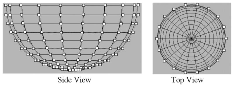
Half-ellipsoid NURBS surface designed to follow the tracked points for one surface of the LV. The surface is composed of 12 levels (horizontal knots) of control points. Each level contains 18 control points radially spaced every 20 degrees. A half-ellipsoid was also created for the surfaces of the RV with 13 levels each containing 24 equally spaced control points.

Fig. 11.

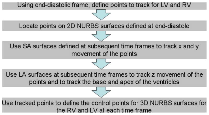
Steps to create time changing NURBS surfaces for the LV and RV based on the tagged MRI data.

To determine if the surfaces predicted for the RV and LV were accurate, we compared them to the actual surfaces as segmented from the gated MRI data. The RV and LV surfaces at each of the 26 time frames were segmented and compared to our predictions based on the tagged MRI analysis. The comparison was done through a distance map. Several points on each ventricular surface were sampled, and the distance to the closest point on the corresponding segmented surface was calculated. Smaller distance measurements indicate a more accurate model prediction.

Once validated, the 3D NURBS surfaces created for the heart ventricles were spline-interpolated in time creating 4D NURBS surfaces representing the cardiac motion. Each 4D NURBS surface is defined by three parametric variables, the two parametric variables u and v defining the 3D surface and t defining the time dimension, by the following equation

$$\mathbf{S}(u,v;t)=\frac{{\displaystyle \sum _{i=0}^n}{\displaystyle \sum _{j=0}^m}{\displaystyle \sum _{k=0}^T}{N}_{k,s}(t)N_{i,p}(u)N_{j,q}(v){\mathbf{P}}_{i,j,k}}{{\displaystyle \sum _{i=0}^n}{\displaystyle \sum _{j=0}^m}{\displaystyle \sum _{k=0}^T}{N}_{k,s}(t)N_{i,p}(u)N_{j,q}(v)}$$ (14)

where P_i,j,k are the control points that define the 4D surface, N_k.s(t), N_{i, p}(u), and N_j,q(v) are the nonrational B-splinebasis functions, and T is the number of time frames.

The multiple surfaces for the LV were additionally spline-interpolated about a new dimension, thickness ρ. The result is a 4D NURBS solid model for the LV with the ability to track any point within the LV myocardium throughout the cardiac cycle. The 4D NURBS solid representation for the LV is defined by the following equation

$$\mathbf{S}(u,v,\rho ;t)=\frac{{\displaystyle \sum _{i=0}^n}{\displaystyle \sum _{j=0}^m}{\displaystyle \sum _{k=0}^T}{\displaystyle \sum _{l=0}^4}{N}_{l,o}(\rho )N_{k,s}(t)N_{i,p}(u)N_{j,q}(v){\mathbf{P}}_{i,j,k,l}}{{\displaystyle \sum _{i=0}^n}{\displaystyle \sum _{j=0}^m}{\displaystyle \sum _{k=0}^T}{\displaystyle \sum _{l=0}^4}{N}_{l,o}(\rho )N_{k,s}(t)N_{i,p}(u)N_{j,q}(v)}$$ (15)

where o is the degree for the interpolation about the thickness parameter which is set to be cubic. The cubic interpolation is between the five surfaces,0 to 4, defined for the LV. For our model, we chose to use cubic NURBS; therefore, the degree parameters p, q, s, and o were set to equal three.

F. Creation of the Atrial Models

Since the tagged MRI data did not fully cover the heart, models for the atria had to be developed using a different set of data. We used MRI data from a normal, healthy patient from the University of Auckland [19] to develop initial models of the atria for the new cardiac model (Fig. 12(a)). The data consisted of short-axis slices spanning the entire length of the heart with a slice thickness of 7 mm. Each slice had a pixel width of 1.17 mm. The images were defined at end-diastole only; therefore, we could not use the data to form motion models for the atria. We used the data to create initial models for the left and right atrium at end-diastole then approximated their motion with simple affine transformations (i.e., translation and scaling) as will be discussed below.

Fig. 12.

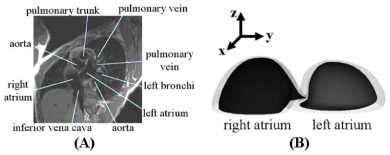
Development of the initial models for the atria. (A) Example slice from the MRI data. (B) 3D view of the surfaces developed for the right and left atrium.

The MRI short-axis images at ED were input into SURF-driver, and the inner and outer walls of the right and left atrium were contoured. The polygon models were then converted into 3D NURBS models. The volumes of the atria models were set to the desired volume for the end-diastolic time frame for a normal, healthy male [20]. This was done by scaling the models equally in the x- and y-directions. The 3D NURBS models for the left and right atria are shown in Fig. 12(b).

The models for the atria were then placed on top of the base of the ventricle models for the end-diastolic time frame (Fig. 13). The control points located at the bottom of each atria model were set to be identical to the control points located at the base of the corresponding ventricle model so the two models would blend together. For example, the model for the inner surface of the left atria was blended with the model for the inner surface of the left ventricle. The models for the atria at ED are shown in Fig. 12(a).

Fig. 13.

Generation of the atria models over the cardiac cycle. (A) Atria models fit to the end-diastolic time frame. (B) Atria models from (A) with the ventricle models at a later time frame (end-systole). The atria models are translated downward according to the longitudinal contraction of the ventricles resulting in (C). The models are then scaled longitudinally keeping the apex of the atria constant. The base of the atria are set to fit the base of the ventricles. The atria are then scaled transversely until they have a particular volume (D).

For each subsequent time frame, the atria models were manipulated to fit the motion of the ventricles and to fit the volume curve for a normal, healthy human male [20] (Fig. 13(b)–(d)). The atria were first translated downward by an amount equal to the longitudinal contraction of the ventricles. The atria were then scaled longitudinally (z) depending on the amount of longitudinal contraction by the ventricles. The origin for this scaling operation was set to be the bottom center of each atria model. The height of the atria was increased by this scaling operation by an amount equal to the amount of longitudinal contraction of the ventricles. Once the atria were scaled longitudinally, the control points located at the bottom of each atria model were then set to the control points of the corresponding ventricle model to blend the two models together. The atria models were then scaled transversely in the x- and y-directions until they fit a certain volume on the predetermined volume curve from a normal male.

III. Results

Our analysis of the tagged data was found to produce accurate models for the right and left ventricles at each time frame. In the distance map comparison, the maximum distance or error was found to be 1.5 mm’s for the LV and 3.4 mm’s for the RV. The errors can be attributed to the tag spacing in the data (7.97 mm’s). The error is higher for the RV since its wall is much thinner than that of the LV and is, therefore, more difficult to follow using the tag lines.

Fig. 14 displays the epi- and endocardial surfaces of the heart surfaces for 3 time frames of the systolic portion of the cardiac cycle. The volumes and muscle mass of each of the heart chambers for the 26 time frames were calculated. The volume curves for the ventricles and atria are shown in Fig. 15. The curves follow the normal pattern for the beating heart. The total myocardial mass was found to be conserved within ±2% while the left ventricular muscle mass alone was found to be conserved within ±5%.

Fig. 14.

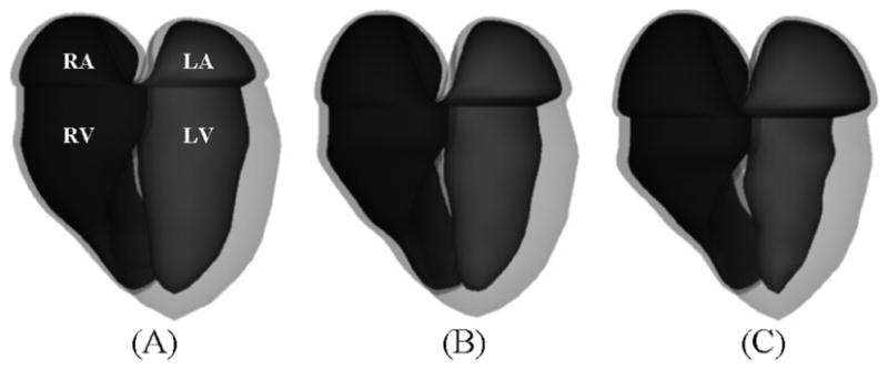
Surface renderings of the epi- and endocardial surfaces of the RA, RV, LA, and LV at (a) end-diastole, (B) mid-systole, and (C) end-systole.

Fig. 15.

Volume curves for the ventricles (A) and atria (B) of the new cardiac model. The volume curves follow the pattern found in an average human.

Fig. 16 shows a surface rendering of the LV with the different surfaces of the LV set at different transparency levels. The same three time frames are shown as in Fig. 14 illustrating the motion of the different layers of the LV. The multiple surfaces of the LV defined at the time frame t were spline-interpolated about the thickness parameter ρ producing a volumetric model of LV at the time t. The volumetric model of the LV S(u,v, ρ; t) is defined by four parametric variables, the parameters u, v, and ρ which define the LV solid, and the parameter t which defines the time frame of the solid. Ten surfaces for the LV at different thickness levels ρ were produced using this method and are shown in Fig. 17 at the time frames for end-diastole, mid-systole, and end-systole. The volumetric model for the LV can be used to follow the motion of any point within the LV myocardium. For example, to track the motion within a voxelized phantom, the u, v, p coordinates of a myocardium voxel would need to be calculated at time frame 0. Once that was done, those coordinates can be used to find the point at subsequent time frames. The phantom; therefore, has the ability to output motion vectors for the cardiac motion at any level of voxelization.

Fig. 16.

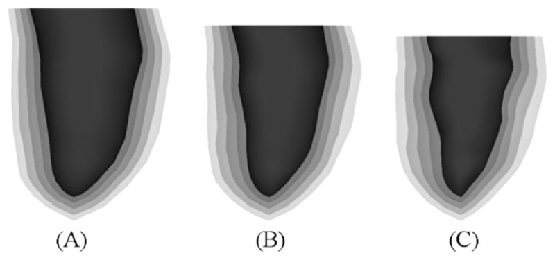
Surface renderings of the five original layers of the LV at (A) end-diastole, (B) mid-systole, and (C) end-systole.

Fig. 17.

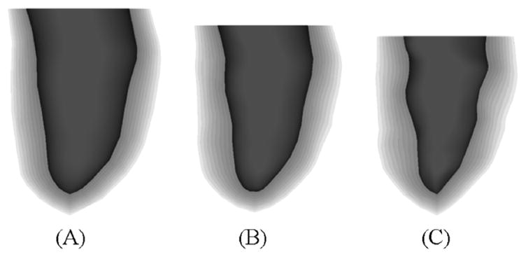
Surface renderings often layers of the LV at (A) end-diastole, (B) mid-systole, and (C) end-systole. The multiple surfaces of the LV were produced by splining the original 5 LV surfaces defined at the time frames about the thickness parameter. Using this technique, an infinite number of surfaces within the LV myocardium can be produced.

Fig. 18 displays a motion analysis of the left ventricle from end-diastole to end-systole. Motion vectors were computed for the five surfaces inside the LV from ED to ES. The motion vectors were computed at three different short-axis slices of the LV: a basal slice, a mid-ventricular slice, and an apical slice. In looking at the side projection of the motion vectors, the longitudinal contraction of the LV can be seen. The base was found to contract 13 mm longitudinally towards a relatively stationary apex. The longitudinal contraction gradually lessons down the length of the LV. Some minor upward contraction can be seen near the apex of the LV.

Fig. 18.

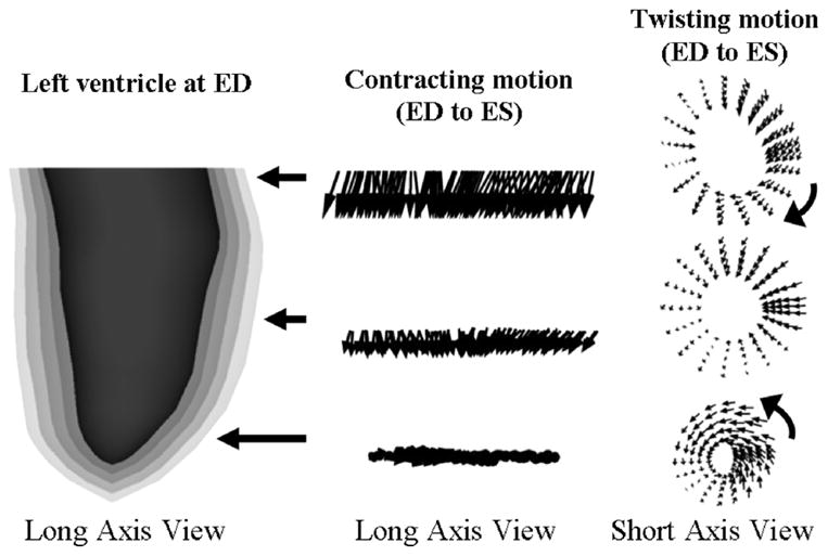
Analysis of the motion of the LV from ED to ES. The LV surfaces defined for ED show the different levels along the length of the LV that were analyzed with motion vectors. The longitudinal contraction of the LV toward the apex can be seen from the motion vectors of the side view. The longitudinal contraction gradually lessons down the length of the LV. Some upward contraction can be seen near the apex of the LV. The “wringing” motion of the LV can be seen in the top view. The LV can be seen to rotate clockwise at the basal region and counterclockwise at the apical region. In the mid-ventricular region, the vectors do not rotate as much. In this region, they eventually switch directions.

The motion vectors also illustrate the radial contraction of the heart. As can be seen from the top view, the motion vectors at all three slices display a radial contraction from diastole to systole. They also involve a twisting motion. The twisting motion at the basal region was found to involve a clockwise rotational movement. The motion vectors for the mid-ventricular region mainly contract without much rotation. At some point in the mid-ventricular region, the motion vectors switch directions eventually resulting in a counterclockwise rotation at the apical region. The outermost surface of the LV was found to twist by a total of 14 degrees from base to apex. The twisting motion gradually increased towards the innermost surface of the LV which twisted by a total of 36 degrees. These motion vectors were found to illustrate the contracting, wringing motion of the heart that has been previously described using tagged MRI [21]–[25].

The enhanced cardiac model was incorporated into the 4D NCAT phantom. The new heart was placed in the chest using the previous model as a guide. The respiratory motion of the heart was setup to be handled as it was previously. The heart simply translates up/down and forward/backward with the motion of the diaphragm. The heart has been shown to move with such rigid body motion as suggested by the following studies [2], [26], [27].

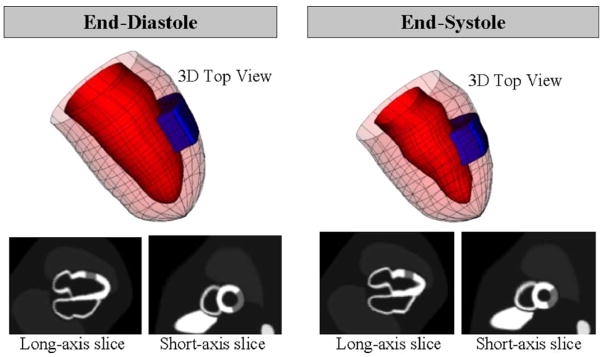
Within the NCAT, the new heart model can be used to simulate 4D data using different imaging applications (Figs. 19–21). Fig. 19 shows the phantom being used to simulate a Tc-99m Sestamibi myocardial SPECT patient study while Fig. 20 shows cardiac gated CT. As was the case with the previous NCAT heart, perfusion defects in myocardial SPECT that result from blocks in the coronary vessels can be simulated in the enhanced cardiac model. The defects are modeled as pie-shaped wedges within the LV myocardium, Fig. 21.

Fig. 19.

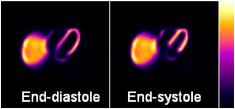
Simulated myocardial SPECT reconstructed short-axis slices using the 4D NCAT phantom with the enhanced cardiac model.

Fig. 21.

Top view and long- and short-axis slice views of a perfusion defect placed in the lateral wall of the LV at end-diastole (left) and end-systole (right).

Fig. 20.

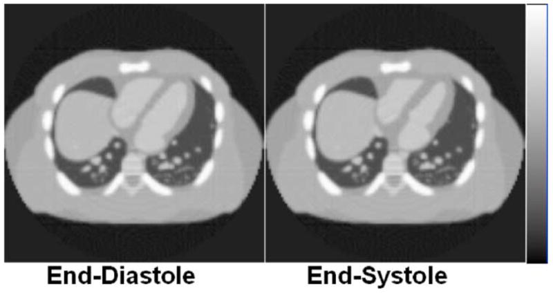
4D cardiac gated CT data simulated using the new 4D NCAT phantom.

Since the heart model is based on a normal patient dataset, the defects will move with the normal cardiac motion. We have developed an application for the NCAT that will allow a user to alter the motion of the defects [28]. The application determines the control points that define the pie-shaped region in the NCAT heart and analyzes the normal motion of them throughout the cardiac cycle. The normal motion is then parameterized in terms of the average regional radial (wall thickening) and longitudinal contractions and for the cardiac twist. These parameters can be scaled to alter the motion of the selected region. The abnormal motion is blended in smoothly through transitional regions with that of the normal myocardium.

IV. Discussion

We enhanced our previous model of the beating heart by using state-of-the-art 4D tagged MRI data. We used an interpolation technique based on NURBS to analyze the full 3D motion of the right and left ventricles from the tagged data. From this analysis, time-dependent 3D NURBS surfaces were created for the RV and LV and a 4D NURBS surface was then fit to the 3D surfaces creating time-continuous 4D NURBS cardiac models.

Since it was based on tagged data, points on the NURBS surfaces of the new 4D cardiac model correspond in time. The only difference between surfaces from one time frame to the next are the location of the control points, and these control points move realistically as if they were actual points on the myocardium. This means that points on a surface can be tracked from one time frame to another. Given a point as defined by its u, v surface coordinates, you can follow that exact point as it moves from different time instances of that surface. This offers a major improvement upon the previous cardiac model [1].

The time-dependent RV and LV surfaces of the new 4D cardiac model were found to realistically illustrate the smooth, contracting, twisting motion of the heart. The longitudinal and radial contraction of the heart as well as the twisting motion were all seen by tracking selected points on the NURBS surfaces. The motion modeled by the 4D NURBS surfaces was found to agree with that determined by the dataset it was based on as well as other studies using tagged MRI data. In addition, the volume curves for the models of the ventricles over the cardiac cycle were found to follow the pattern for a normal beating heart.

We created multiple 4D surfaces for the left ventricle spanning its entire volume. These were used to create a 4D NURBS solid model for the LV with the ability to represent the motion of any point within the volume of the LV myocardium at any point during the cardiac cycle. With the volumetric model of the LV, we can now more realistically model myocardial defects located within the volume of the LV myocardium since the motion of the model is more realistic and complete. Also, the phantom can be used to provide a known truth for the motion of any point within the myocardium. Such ability is extremely useful to evaluate reconstruction algorithms that estimate and correct for the cardiac motion.

To complete our heart phantom, we created models for the atria based on MRI data from the University of Auckland. The MRI data was defined for end-diastole only. We used the data to create initial models for the atria at end-diastole then approximated their motion with simple affine transformations using a volume curve for a normal human male as a guide. The 4D models of the atria developed here are not as realistic as the ventricles since their motion was not based on gated patient data. However, accurate modeling of the atria is not as important for SPECT simulation studies since the main area of concern in myocardial SPECT is the ventricular myocardium.

The cardiac phantom created in this work was based on the tagged data of one normal patient. Our ultimate goal is to create many different patient variations (normal and diseased states). We are currently analyzing several sets of tagged MRI patient data (normal and abnormal) using the techniques presented in this paper. Based on this analysis, we will, at the minimum, be able to create a series of heart models to insert into the 4D NCAT. Depending on how the anatomy and motion varies from patient to patient, we may be able to parameterize the heart so that we can create many variations from a single or a handful of template models.

We are also looking at combining the heart phantom created in this work with a finite-element (FE) mechanical model of the LV. The advantage to FE methods is that they provide a physiological basis upon which to model motion abnormalities indicative of cardiac disease. As mentioned previously, abnormalities can be simulated in the heart model developed here, but are defined by simply scaling the motion down in the user-defined defect regions. In the FE mechanical model, the material properties can be adjusted to more realistically simulate regional motion defects [29]. FE modeling is disadvantageous in that it is more computationally intense. We are currently investigating how best to combine our different modeling (FE and tagged MRI-based) approaches.

V. Conclusions

With its ability to accurately simulate the internal and external motion of the heart, the enhanced cardiac model developed in this work offers a great improvement over our previous NCAT model. It has great potential to be used in the study of cardiac imaging and the effects of cardiac motion in medical images.

References

- 1.Segars WP, Lalush DS, Tsui BMW. A realistic spline-based dynamic heart phantom. IEEE Trans Nucl Sci. 1999 Jun;46(3):503–506. [Google Scholar]
- 2.Segars WP. Ph.D. dissertation. Univ. North Carolina; Chapel Hill: 2001. Development of a New Dynamic Nurbs-Based Cardiac-Torso (NCAT) Phantom. [Google Scholar]
- 3.Axel L. Efficient method for selecting cardiac magnetic resonance image locations. Invest Radiol. 1992;27(1):91–3. doi: 10.1097/00004424-199201000-00018. [DOI] [PubMed] [Google Scholar]
- 4.Axel L, Dougherty L. MR imaging of motion with spatial modulation of magnetization. Radiology. 1989;171:841–845. doi: 10.1148/radiology.171.3.2717762. [DOI] [PubMed] [Google Scholar]
- 5.Axel L, Dougherty L. Heart wall motion: Improved method of spatial modulation of magnetization for MR imaging. Radiology. 1989;172:349–350. doi: 10.1148/radiology.172.2.2748813. [DOI] [PubMed] [Google Scholar]
- 6.Bolster B, McVeigh E, Zerhouni E. Myocardial tagging in polar coordinates with striped tags. Radiology. 1990;177:769–772. doi: 10.1148/radiology.177.3.2243987. [DOI] [PMC free article] [PubMed] [Google Scholar]
- 7.McVeigh E, Zerhouni E. Noninvasive measurement of transmural gradients in myocardial strain with MR imaging. Radiology. 1991;180:677–683. doi: 10.1148/radiology.180.3.1871278. [DOI] [PMC free article] [PubMed] [Google Scholar]
- 8.Mosher T, Smith M. A DANTE tagging sequence for the evaluation of translational sample motion. Magn Reson Med. 1990;15:334–339. doi: 10.1002/mrm.1910150215. [DOI] [PubMed] [Google Scholar]
- 9.Zerhouni E, et al. Human heart: Tagging with MR imaging – A method for noninvasive assessment of myocardial function. Radiology. 1988;169:59–63. doi: 10.1148/radiology.169.1.3420283. [DOI] [PubMed] [Google Scholar]
- 10.McVeigh E. MRI of myocardial function: Motion tracking techniques. Magn Reson Imag. 1995 doi: 10.1016/0730-725x(95)02009-i. to be published. [DOI] [PubMed] [Google Scholar]
- 11.Declerck J, et al. Left ventricular motion reconstruction from planar tagged MR images: A comparison. Phys Med Biol. 2000;45(6):1611–32. doi: 10.1088/0031-9155/45/6/315. [DOI] [PMC free article] [PubMed] [Google Scholar]
- 12.Ozturk C, McVeigh ER. Four-dimensional B-spline based motion analysis of tagged MR images: Introduction and in vivo validation. Phys Med Biol. 2000;45(6):1683–1702. doi: 10.1088/0031-9155/45/6/319. [DOI] [PMC free article] [PubMed] [Google Scholar]
- 13.Guttman M, Zerhouni E, McVeigh E. Analysis of cardiac function from MR images. IEEE Comput Graph Appl. 1997;17:30–38. doi: 10.1109/38.576854. [DOI] [PMC free article] [PubMed] [Google Scholar]
- 14.Piegl L. On NURBS: A survey. IEEE Comput Graph Appl. 1991;11:55–71. [Google Scholar]
- 15.Piegl L, Tiller W. The Nurbs Book. New York: Springer-Verlag; 1997. [Google Scholar]
- 16.Press WH, et al. Numerical Recipes in C. Cambridge, U.K: Cambridge Univ. Press; 1988. pp. 343–352. [Google Scholar]
- 17.Moody D, Lozanoff S. A practical computer program for generating three-dimensional models of anatomical structures. Proc. 14th Annu. Meeting Amer. Assoc. Clinical Anatomists; Jul. 8–11, 1997. [Google Scholar]
- 18.McNeil R. Rhinoceros. Seattle, WA: Rhino3d.com; 1998. [Google Scholar]
- 19.Thrupp S. Cardiac MRI Anatomical Atlas: An Introduction to Anatomy [Online] Available: http://www.scmr.org/education/atlas/intro/index.html.
- 20.Guyton A, Hall J. Textbook of Medical Physiology. 9. Philadelphia, PA: Saunders; 1996. [Google Scholar]
- 21.Park J, Metaxas DN, Axel L. Analysis of left ventricular wall motion based on volumetric deformable models and MRI-SPAMM. Med Imag Anal. 1996;1:53–71. doi: 10.1016/s1361-8415(01)80005-0. [DOI] [PubMed] [Google Scholar]
- 22.Park J, Metaxas DN, Axel L. Quantification and visualization of the 3D nonrigid motion of the left ventricle. Proc SPIE Medical Imaging Conf (Physiology and Function) 1997:177. [Google Scholar]
- 23.Park J, et al. Deformable models with parameter functions for cardiac motion analysis from tagged MRI data. IEEE Trans Med Imag. 1996;15:278–289. doi: 10.1109/42.500137. [DOI] [PubMed] [Google Scholar]
- 24.Young A, et al. Tracking and finite element analysis of stripe deformation in magnetic resonance tagging. IEEE Trans Med Imag. 1995;14:413–421. doi: 10.1109/42.414605. [DOI] [PubMed] [Google Scholar]
- 25.Young AA, Axel L. Three-dimensional motion and deformation of the heart wall: Estimation with spatial modulation of magnetization – A model-based approach. Radiology. 1992;185(1):241–247. doi: 10.1148/radiology.185.1.1523316. [DOI] [PubMed] [Google Scholar]
- 26.Wang Y, Riederer S, Ehman R. Respiratory motion of the heart: Kinematics and the implications for the spatial resolution in coronary imaging. Magn Reson Med. 1995;33:713–719. doi: 10.1002/mrm.1910330517. [DOI] [PubMed] [Google Scholar]
- 27.Segars WP, Chen GTY, Tsui BMW. Modeling respiratory motion variations in the 4D NCAT phantom. Proc. IEEE Nuclear Science Symp./Medical Imaging Conf; Honolulu, HI. 2007. [Google Scholar]
- 28.Segars WP, Lee TS, Tsui BMW. Simulation of motion defects in the 4D NCAT cardiac model. J Nucl Med. 2003;44(5):142P–142P. [Google Scholar]
- 29.Veress AI, et al. Normal and pathological NCAT image and phantom data based on physiologically realistic left ventricle finite-element models. IEEE Trans Med Imag. 2006;25(12):1604–16. doi: 10.1109/tmi.2006.884213. [DOI] [PubMed] [Google Scholar]