Individual histories and selection in heterogeneous populations

Abstract

The strength of selection in populations has traditionally been inferred by measuring changes in bulk population parameters, such as mean reproductive rates. Untangling the effect of selection from other factors, such as specific responses to environmental fluctuations, poses a significant problem both in microbiology and in other fields, including cancer biology and immunology, where selection occurs within phenotypically heterogeneous populations of cells. Using “individual histories”—temporal sequences of all reproduction events and phenotypic changes of individuals and their ancestors—we present an alternative approach to quantifying selection in diverse experimental settings. Selection is viewed as a process that acts on histories, and a measure of selection that employs the distribution of histories is introduced. We apply this measure to phenotypically structured populations in fluctuating environments across different evolutionary regimes. Additionally, we show that reproduction events alone, recorded in the population’s tree of cell divisions, may be sufficient to accurately measure selection. The measure is thus applicable in a wide range of biological systems, from microorganisms—including species for which genetic tools do not yet exist—to cellular populations, such as tumors and stem cells, where detailed temporal data are becoming available.

Measuring the strength of selection in populations is fundamental to any quantitative description of evolution. In laboratory experiments, populations of microorganisms can be propagated for many generations, in constant or fluctuating conditions, and adaptation of growth rates and other characteristics can be measured (1). Adaptation of the population as a whole may arise from individual responses, such as sensor-mediated changes in gene expression activating specific pathways that are beneficial in certain conditions. Likewise, it can result from selection acting on existing, heritable phenotypic and/or genotypic differences between individuals [e.g., as in antibiotic persistence (2), bacterial sporulation and competence (3), and phase variation (4)]. In reality, both individual responses and population-level selection occur concurrently, and the adaptation of the population results from the mixture of these two forces. It should be highly informative therefore to characterize the effective strength of selection in experimental evolution. Such measurement would identify specific environmental conditions that require adaptation via selection, as well as those for which an organism already possesses suitable genetic pathways of response. It could, in principle, be predictive as well of what an organism can easily adapt to via selection, and what might be more difficult.

In population genetics studies, the existence of selection and its strength are indirectly inferred from analysis of existing genetic variation in populations (5). In experimental evolution, where one hopes to directly observe selection in action, selection measurements have been based on changes in bulk population growth rate and on the variance of reproductive rates (1). The insight of Fisher (6) was to partition the change in the population growth rate into two terms, the first due to changes in allele frequencies, and the second due to changes in environmental conditions (7–10). The first term was defined as the measure of selection and was proven to be equal to the population’s variance of fitness. While mathematically valid, and intuitively appealing, the theorem is difficult to apply directly to experiments because it neglects the effect of mutations, as well as other aspects of population structure such as phenotypic heterogeneity, specific responses, and environmental fluctuations, all of which are relevant on time scales of laboratory experiments.

Recently, detailed temporal information about individuals in microbial populations has become available (3, 11–15) Using gene-specific fluorescent reporters, video microscopy, and automated image analysis, one can follow each “history,” i.e., temporal sequences of all reproduction events and all phenotypic changes of a given individual and of its ancestors (16). Cell lineage data are also becoming available in other systems, including hematopoietic stem cells (17) and carcinoma cell lines (18). Such detailed data should allow one to proceed beyond the classical measures of selection, both in microbiology and in other fields such as cancer biology where selection occurs within phenotypically heterogeneous populations of cells (19, 20). We introduce here a theoretical framework that takes full advantage of individual-level temporal data that is typical of recent experiments, while simultaneously maintaining the intuitive aspects of Fisher’s and Price’s formulations of population evolution (6, 21). Key to our approach is the shift of focus from individual organisms to individuals’ histories.

What needs to be measured regarding selection? Selective differences are certainly measurable, when sufficiently large, so this poses no fundamental problem. How such differences propagate to the population level, however, can depend strongly on mutation rates, phenotypic heterogeneity, environmental fluctuations, population sizes, and demography. Finding the key measurements of this process is thus at the heart of what selection means as a biological concept. To avoid a potentially subjective resolution of this problem, we introduce here a thought experiment that provides a conceptual basis for measuring selection, which is inspired by similar problems in the physical sciences. To gauge the importance of thermal fluctuations, for example, for the behavior of a physical system, such as a solution, or a crystal, the natural approach is to change temperature and measure how the system responds. Similarly, to gauge the importance of selective differences for the behavior of a population, it seems natural to change the relative magnitude of those differences and measure how the population responds. We imagine an experiment A, in which a population is tracked over many generations with controlled environmental fluctuations. Simultaneously, an almost identical experiment B is performed, with precisely the same temporal changes of environment, except that reproduction rates (fitness values) of all individuals are multiplied by a constant value β, close to 1, which we call the historical conditions factor. We then compare any measurable quantity between experiments A and B, with the difference measuring the importance, or effective strength, of selection for the given quantity.

Importantly, in experiment B, we perturb fitness values very slightly. In this way, we assess the effective strength of selection in conditions that are as close as possible to the conditions of the experiment itself. We stress that experiment B is most likely not feasible in any given system, and we introduce it here as a gedanken experiment, not to be performed. Remarkably, however, we will demonstrate that the response of the population to the change of fitness is completely determined by the distribution of histories in experiment A alone, and may be measured without performing experiment B. We will then show that the fitness of individuals measured over their history—the historical fitness—is a key quantity: The response of its mean to the change of β is precisely equal to its variance. The result, which is reminiscent of Fisher’s theorem, is nevertheless exact even in the presence of mutations, phenotypic heterogeneities, and fluctuating environments.

Theoretical Approach

Population Dynamics—Standard Formulation.

We consider a model of a heterogeneous, asexual population in which individuals have different, discrete phenotypes, indexed by i, which reproduce with different rates that may depend on fluctuating environmental conditions, . Individuals can switch phenotypes according to a set of rates , which denotes the rate of switching from phenotype j to phenotype i in environment . We define , so the diagonal elements are the total rate of switching out of each phenotype. The potential dependence of switching rates on the environmental state allows for both stochastic and response-mediated switching to be modeled (22); switching rates may also model mutational or epigenetic rates.

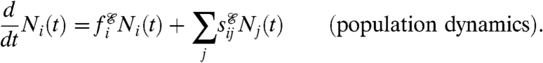
The term “phenotype” throughout this paper refers to both genetic and nongenetic diversity, and the term “fitness” will be synonymous with individual reproductive rates, i.e., the potential for reproduction, whereas reproduction events are the result of a fitness-dependent stochastic process. While this stochastic process is cumbersome to write explicitly (see SI Text), its expected behavior is given by the following equations for N_i(t), the expected number of cells with phenotype i at time t:

From the expected total population size, , we obtain the frequency of phenotype i in the population: n_i(t) ≡ N_i(t)/N(t). It follows that the population mean fitness, 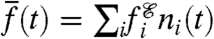, is equal to the bulk population growth rate, , which is often measured in evolution experiments. The average value of this quantity over the entire experiment, , or the long-term growth rate, converges to (1/t) log N(t), for large t in exponentially growing populations.

Population Dynamics—History Formulation.

We recast the above model in a formulation that uses individual histories as its basis. We begin as in ref. 23 by considering a scenario in which a population of cells is observed for a total time t, and an individual cell is traced back by recording for all times t^′ < t its historical phenotypic states, σ(t^′) (see Fig. 1). When we refer to the entire history, we will denote it by σ, reserving the notation σ(t^′) for the historical phenotypic state at time t^′. The history formulation describes expectations of historical quantities, taken over the stochastic process of reproduction and switching. In bounded populations, such expectations are measured by sampling independent histories (see Methods).

Fig. 1.

Overview of the history formulation. An example of a growing population is shown in which individuals can be in two different phenotypic states. The population’s lineage tree is colored to indicate individuals’ phenotypes (green or red). The environment is indicated by the background color. In each type of environment (green or red), the adapted phenotype, i.e., the fastest reproducing one, matches the environment’s color.

Two mathematical quantities play a key role: the integrated, historical fitness, H_σ, and the a priori probability, P_σ, both of which depend on the environment . The quantity H_σ is found by integrating the cell’s reproduction rate over time (see Fig. 1) and depends on the cell’s entire phenotypic history, σ, but not explicitly on details of the cellular mechanisms that underly the phenotypic changes:

The quantity P_σ is found by computing the probability that a single cell exhibits the temporal sequence σ of phenotypic switches and depends on the individual-level cellular mechanisms, but not on the reproduction rates of phenotypes. The expression for P_σ depends on parameters (see SI Text), but its precise form will not be needed here.

The histories observed in any given experiment depend on a competitive interplay between their a priori probability, which is determined by individual-level mechanisms, and selection, which acts at the population level. The effect of selection is to amplify histories exponentially according to their historical fitness. The expected number of cells with a given history σ is therefore given by its a priori probability, P_σ, times the exponential factor e^βH_σ (for now we can think of β being equal to 1). The total expected number of cells at time t, descended from a single initial cell, is found by summing the quantity P_σe^βH_σ over all possible histories:

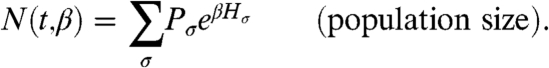In the presence of selection, histories that would normally be rare (according to P_σ) can become common in the population. The frequency of a history is denoted by x_σ, defined as the expected number of cells with history σ divided by the total number: x_σ ≡ P_σe^βH_σ/N(t,β).

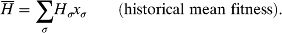
Analogous to the population mean fitness, in the history formulation we define the mean fitness of histories, :

Selection and Histories.

To decouple selection from other effects, the history formulation allows us to change β and measure the response of any quantity. We compute how a change of β affects the frequency of histories,

[1]

and how the change of β affects the mean historical fitness,

Returning to the thought experiment, the left-hand side above corresponds to the result of comparing experiment B to experiment A. Evaluating the result at β = 1 (i.e., a tiny perturbation of fitness), the right-hand side is then precisely the historical fitness variance in experiment A. Therefore we can assert that the result of the thought experiment is, in fact, measurable without performing experiment B.

The use of the derivative with respect to β to measure the effective strength of selection is natural, as we have argued based on an analogy with physical systems (see Discussion). Derivatives of quantities other than , however, may, in principle, be useful as well. For example, the population mean fitness is another natural candidate, which can be written as , whose derivative is found using Eq. 1 to be . Here, we will use the historical fitness variance per unit time,

as the measure of selection. We make this choice due to the formal similarities between and Fisher’s result, as well as the direct applicability of to experiments, which will be shown below.

We can interpret the historical fitness relation in terms of the behavior of histories. Eq. 1 shows that upon a change of β, frequencies of histories change as though the histories themselves were the fundamental replicating entities. Histories with larger fitness will benefit from a change in historical conditions exponentially more than histories with smaller fitness. If histories in the population have similar values of H_σ, the change in historical conditions benefits them equally, and the mean historical fitness, , changes minimally. Conversely, if the distribution of H_σ is broad, the change in historical conditions benefits those histories with high H_σ disproportionally, and the change in the mean historical fitness is large. The intuition behind Fisher’s theorem is therefore applicable to histories as replicating entities.

Results

To investigate the behavior of histories across different evolutionary regimes, we now specialize the general model. Individuals will be assumed to have two phenotypic states, each adapted to two different environments. Environmental changes occur here periodically, with period τ, and individuals can switch phenotype in a way that is either stochastic (switching randomly between the phenotypes) or responsive (switching specifically to the adapted phenotype, i.e., sensing). Adapted individuals reproduce with rate f_a, and nonadapted individuals at a lower rate f_na. Rates of stochastic and responsive switching are given by s and s_r, respectively. The model allows for organisms that employ a mixture of stochastic and responsive switching, organisms that sense and respond but might make errors, as well as pure stochastic (s_r = 0) and pure responsive (s = 0) organisms.

We simulate these stochastic and responsive models, keeping track of individual histories, for both normal (β = 1) and improved (β = 1.1) historical conditions. Upon a change of historical conditions, the change in observed in simulation is used to estimate , as shown in Fig. 2A. Even with very few histories depicted in Fig. 2, it is apparent that the larger the historical fitness variance in normal conditions, the larger the increase in mean fitness upon improved conditions (see also Fig. S1). To verify the relation quantitatively, Var(H_σ) must be estimated accurately (as in Fig. 3 below), which requires hundreds of independent histories (see Discussion).

Fig. 2.

Individual histories in two-phenotype models. (A) Individual histories are shown for responsive and stochastic switching models, for normal and 10% improved historical conditions. For each model and historical condition, three independent simulations were run, and a randomly chosen individual history is shown from each simulation (colored segments), with the same color scheme as in Fig. 1. Tick marks display cell divisions. Temporal intervals during which an individual was in the adapted state are shown (gray segments), and the percent of time spent in the adapted state is indicated. Parameters used were s = 0, s_r = 1, f_a = 0.88 (responsive), and s = 0.01, s_r = 0, f_a = 1 (stochastic); τ = 10 and f_na = 0 in both cases. The parameters were chosen such that for both models, the analytically computed value of is the same (); simulation results reflect this, with slight deviations due to the small number and short length of histories shown. Direct estimates of are in good agreement with analytically computed values (responsive) and (stochastic). (B) Histories in normal historical conditions from A are shown with historical divisions only (phenotypic states and environments are not displayed). Selection here is stronger for slow stochastic switching, seen via its high value of and non-Poissonian (patchy) distribution of historical divisions.

Fig. 3.

Dependence of on the environmental duration τ for the two-state models of stochastic and responsive switching described in the text. Fitness values for all models shown are f_a = 1 and f_na = 0.1. The dashed line in all panels is the curve 1/τ, shown for reference. All rates, including f_a, f_na, s, s_r, and , are given in arbitrary units of 1/time, with τ shown in the same units of time. (A and B) Analytically computed curves are shown for pure stochastic switching (A), for given values of s, and for responsive switching (B), for given values of s_r with s = 0.1. (C) Measurements of (filled circles) using statistics of cell divisions from stochastic population simulations are compared with analytically computed values (solid curve). Blue: pure stochastic switching with s = 0.01; magenta: responsive switching, with s_r = 0.95 and s = 0.05. Each point is an average over 100 estimates of that were generated (see Methods); the bars on three representative points show the standard deviation of the estimates. The blue curves in A and C are identical.

The value of can be computed exactly (see Methods), for any instance of the given model, over the entire range of fluctuation periods τ (Fig. 3). The strength of selection measured by depends on both the nature of individual behavior and the period of environmental fluctuations. For stochastic switching (Fig. 3A), a pronounced peak in (note the logarithmic scale) is present at values of τ significantly larger than the generation time. For responsive switching (Fig. 3B), the curve is shifted downward relative to the pure stochastic case, and its peak becomes less pronounced. The existence and meaning of these peaks can be understood qualitatively (see Discussion), by considering the relevant population dynamics. Likewise, asymptotic behaviors of these curves can be derived in the limits of fast (τ ≪ 1) and slow (τ≫1) environmental fluctuations (see SI Text). We note that clearly distinguishes between stochastic and responsive switching via the location and magnitude of the peak with respect to the dashed line 1/τ. Also in agreement with our expectation, increasingly slow responsive switches (s_r ≪ 1) behave increasingly like pure stochastic switches, as their peak crosses this line. Fig. S2 presents additional plots for cases of fast stochastic switching, and switching with asymmetric fitness values.

The definition of based on detailed phenotypic histories seems to imply that measurement of this quantity directly from experimental populations (or in this work, directly from simulated ones) would require information about the internal phenotypic states of cells. Surprisingly, however, we find that can in some cases be inferred accurately using only the distribution of cell divisions over individual histories. Indeed, visual inspection of Fig. 2B shows that for slow stochastic switching, for which the effective selection strength is large, the pattern of cell divisions across the histories is strikingly nonuniform, with patches of cell division separated by empty intervals (in contrast to responsive switching).

This observation is explained by noticing that the number of cell divisions observed in a history σ is a random variable D_σ whose statistical properties depend on the cell’s historical fitness H_σ. Variance in D_σ between histories results from two sources: (i) variance of the historical fitness of different cells, i.e., Var(H_σ), and (ii) variance of the cell division process itself. The latter is given by , for the case in which the times between cell divisions are exponentially distributed random variables. This results in the following measurement formula (see SI Text): .

By performing independent replicate experiments, in which all cell divisions are recorded, may thus be measured using the difference between the variance and the average number of cell divisions over independent histories, with a large difference resulting in the patchiness observed in Fig 2B. Fig. 3 depicts the results of simulations, in which we measured from cell division statistics (filled circles), showing an excellent agreement with values expected from exact calculations (solid curves). With a modification, the same approach may be used to measure also in other cases for which cell division times are not exponentially distributed (e.g., for gamma distribution, see SI Text). Thus, it seems that could in some cases be measurable directly by using cell divisions as a reporter on the underlying historical fitness and would not necessarily require knowledge of the internal states of cells.

Discussion

In laboratory experiments, the change in bulk growth rate over time, , has often been used to detect the presence of selection. In the absence of phenotypic switching of any kind (i.e., ), this change is equal to the population fitness variance, , i.e., a simple version of Fisher’s theorem. Switching introduces a major deviation from this result (given in SI Text) with several consequences: (i) changes in may no longer reflect the action of selection, (ii) the population fitness variance may no longer be a measurable quantity in bulk, and (iii) even if measurable, a large fitness variance may no longer imply an increase of . Crucially, in experiments it is difficult to determine whether any or all of these consequences are in effect. Fundamentally, phenotypic switching (responsive and/or stochastic) entangles the action of selection and of individual response in a manner that appears to be difficult to separate via bulk measurements.

We consider a few examples to illustrate the above possibilities. As an example of case (i), we consider pure responsive switching, wherein cells change their internal state upon a change of environment, e.g., a change of carbon source. Measurement of right after the change results in a low value because cells have not yet responded. Measurement of at later times will be positive, while cells in the population respond to the change. As more cells respond, will decay back toward zero. If cells respond with a rate that is faster than their division rate, measured changes in will be due largely to individual responses, rather than selective differences, and will reflect individual-level response instead of population-level selection.

For cases (ii) and (iii), we consider fast stochastic switching, i.e., cells that switch phenotypes with rates comparable to the cell division rate. To measure fitness variance, one would typically initiate many clones, measure the bulk growth rate for each, and find the variance. However, if cells switch phenotypes quickly, each clone will rapidly reestablish the equilibrium mixture of phenotypes. Growth rate measurements within clones must then be made in the first few generations, which in general requires measuring individual histories, rather than bulk growth rates. Even if such measurements are feasible in bulk in specific systems (e.g., if specific labels of phenotypes are available), it is easy to see that the variance of fitness in such cases is not necessarily measuring any kind of selection. The variance is due to the fact that cells change phenotype faster than they divide. As these few examples show, bulk population measurements, such as and Var(f), confound individual-level mechanisms with population-level selection.

The history formulation provides a unifying framework to describe population dynamics at the individual level and can untangle selection from the multitude of individual-level behaviors that affect bulk measurements. To relate historical quantities with well-established intuition regarding population dynamics, we discuss the behavior of in several important regimes. First, we consider the dynamics of a population “climbing” a fitness peak, e.g., when switching rates correspond to mutational rates. Before reaching the peak, because mutations are available that increase fitness. Upon reaching the peak, further increase of the mean fitness is not possible, and tends to zero. The population reaches the so-called mutation-selection balance, wherein the fraction of the population “falling off” the peak (due to mutation) is precisely balanced by the excess rate of cell divisions on the peak. At such equilibrium, measurement of yields a nonzero value. This may be seen in its asymptotic behavior as τ → ∞ in Fig. 3A, which via direct calculation (see SI Text) yields , with Δf = f_a - f_na, and s ≪ Δf, i.e., as switching (mutation) rate s increases, selection plays an increasingly greater role in keeping the population on the peak.

Importantly, we find that the value of at a fitness peak decreases as the fitness difference Δf (the benefit of being on the peak) increases. This may seem counterintuitive at first because increasingly large fitness differences are typically thought of as increasingly strong selection. In such cases, however, the time scale over which selection acts is increasingly short (order of 1/Δf), because nonadapted variants are rapidly eliminated. The measure is therefore sensitive to the proportion of time the population structure is affected by selection. We can relate this as well to behavior in fluctuating environments, by considering selective sweeps, i.e., temporal intervals during which selection amplifies adapted variants to high frequency. If large fitness differences exist but occur rarely, sweeps will seldom occur, completing quickly when they do, and will record a relatively small value, e.g., when τ in Fig. 3A is large. Alternatively, if fitness differences are very small, sweeps occur rarely for a different reason—many individuals are competing to sweep [a phenomenon known as clonal interference (see, e.g., ref. 24)]—and is likewise small. This can be seen for small values of τ in Fig. 3A, when the environment changes multiple times in a single generation, and all cells have similar fitness values on average over their life spans. It is thus only in the intermediate range of τ, between rare and frequent fluctuations, that exhibits large values, due to the high frequency of sweeps as a fraction of the total time of experiment.

Although the history formulation was derived assuming an unbounded population size, it is applicable for bounded populations, as seen by simulation results that closely match theoretical predictions (Fig. 3C). This is not the result of a coalescent process approach (25), i.e., a detailed calculation of the distribution of times to common ancestry in a single finite population, subject to a specific population process. Rather, the agreement is a consequence of the fact that whereas unbounded populations, in principle, have a wider distribution of H_σ than bounded ones, in practice both distributions are dominated by the same class of optimal histories, with exponentially suppressed deviations. These histories optimize a trade-off, spending excess time in fit phenotypes without sacrificing excessively their a priori probability, thus multiplying fastest; histories deviating from this optimum are exponentially outcompeted. Averaging over independent histories in bounded populations, or over replicate experiments, probes this distribution without bias and allows accurate estimation of expectations such as .

To get an order-of-magnitude sense of the amount of data and time needed to estimate , Fig. 3C shows the variance of estimates that use 1,000 independent histories of length 100 time units, e.g., at τ = 10 units, estimates have a 10% accuracy. To convert to real time, the adapted phenotype’s growth rate of 1 per unit time is matched to a realistic growth rate for bacteria of 2 per hour (this corresponds to a doubling time of approximately 20 min), i.e., the time unit is half an hour. Each independent history is therefore about two days long and experiences a change of environment every 5 h. Each population in simulation is limited to a size smaller than 1,000 cells. An entire experiment that tracks hundreds of populations could thus be performed in a microfluidic device on a single microscope in two days. We note that while the direct tracking approach is eminently feasible for cellular populations, it will be difficult in large multicellular organisms. We do not rule out the possibility of applying the history formulation in such cases, because alternative approaches may eventually be found to infer the historical reproductive success of organisms.

A very general description of evolutionary change in populations of replicators, known as the Price equation (21), states that the change in the population average of any trait value is given by the covariance across the population between trait values and fitness [if trait values themselves can change in time, additional terms are necessary (26)]. In the history formulation, one can derive (see SI Text) the following Price equations:

[2]

where we suppress the superscript on fitness values for notational ease. We can see that when β is varied, histories are the replicators, and their fitness is given by H_σ. Viewed in the Price formulation, one trait value is f_σ(t), i.e., the temporal growth rate of the cell σ at time t, and hence is given by Cov(f_σ(t),H_σ). The historical fitness relation is likewise a Price equation, because if historical fitness itself is taken as a trait value, is given by the covariance of the trait value, H_σ, and its fitness, H_σ, i.e., by Var(H_σ). When time is varied, rather than β, cells rather than histories are the replicators, and their fitness is given by βf_σ(t). A cell’s historical fitness H_σ is then a trait value and obeys the Price equation, with additional terms appearing because the trait value itself changes temporally.

The general idea of changing β in the population is similar to changing temperature in a physical system. The expression for population size as a sum over histories is precisely a partition sum of Boltzmann factors, with β playing the role of the inverse temperature. Mappings between population dynamics and statistical physics have a long history (23, 27–32), dating back to an imaginative analogy by Fisher (6) between evolution and thermodynamics. Demetrius introduced the idea of entropy in the context of individual lineages, by examining a model of age-structured populations (27). Derrida and Peliti introduced the connection between evolutionary dynamics and the theory of disordered systems, such as spin glasses (29). Spatial fluctuations in growing populations were considered via analogy with convection by Nelson and Shnerb (30). Recently, several groups have described evolution of allele frequencies in populations using physical analogies, both from equilibrium and nonequilibrium points of view (32, 33).

To characterize the interplay between mutation and selection, Baake and co-workers introduced the idea of the ancestral distribution of types along histories (23) and later, using the theory of large deviations, considered competitions between lines of descent having different ancestral distributions in a constant environment (reviewed in ref. 34). As an alternative to large deviations, we previously presented a mapping between population dynamics and the theory of heteropolymers, which maps polymer conformations to histories, and predicted a population phase transition that occurs as environmental durations τ change (31). More recently, Mustonen and Laessig considered temporal trajectories of the frequency distribution, n_i(t), as realizations of nonequilibrium dynamics in finite populations, and introduced a measure of population adaptation called the fitness flux, Φ, which considers the rate of frequency changes multiplied by their fitness value (33). Because this approach is based on population trajectories, rather than individual histories, intriguing possibilities exist of bridging these two viewpoints.

The most important departure between the history formulation described here and previous studies is the introduction of the historical fitness relation as a tool to measure selection. Remarkably, at least in the simple cases we have examined, enough information exists in the distribution of cell divisions along individual histories for direct measurement of , without knowledge of individuals’ phenotypic states and fitness values. This opens possibilities of precisely measuring the effect of selection in controlled experiments involving populations of microbes, other organisms, or individual cells.

Methods

Analytical Calculation of .

The distribution of H_σ (evaluated at β = 1) has the following cumulant generating function: . If κ_n is the nth cumulant of the historical fitness distribution, then we have

[3]

i.e., is the cumulant generating function of historical fitness. To evaluate , we find , take two β derivatives, and evaluate at β = 1. For the periodic case of two environments considered in the text, we define the matrices A₁ and A₂ by (where δ_ij is the Kronecker delta symbol), and find , where λ₁ denotes the maximum eigenvalue of the matrix, as in ref. 35. For the case of two-by-two matrices, this is computable exactly, as is (evaluated at β = 1), shown in Fig. 3.

Simulation Method and Bounded Populations.

Stochastic simulations of population dynamics were performed, in which all cell divisions were recorded, and all individuals’ histories were stored. We used the two-state model described in Results, simulating the continuous-time stochastic processes for a small population as in ref. 35. To avoid double counting, each division is assigned arbitrarily to one and only one lineage (see SI Text). Each time the population size reached 1,000 cells, only 100 randomly chosen cells were allowed to continue. Simulation length was 3,000 time units, and data from n_runs = 1,000 simulations were used to obtain each data point in Fig. 3C. The number of histories present in a bounded population comprises a tiny fraction of the total number of possible histories over any time interval. These histories are correlated due to common descent. To obtain independent histories for averaging, from each of the n_runs simulations a single individual history and a time window of size t_w were chosen randomly. The measurement formula for was applied to the n_runs windows (with t = t_w), to obtain one estimate of . The entire random windowing process was repeated 100 times (i.e., resampling from the same simulation data), and the estimates of were averaged, to obtain the final estimate. The results shown in Fig. 3 used a window size of t_w = 100 time units.

References

- 1.Elena S, Lenski R. Evolution experiments with microorganisms: The dynamics and genetic bases of adaptation. Nat Rev Genet. 2003;4:457–469. doi: 10.1038/nrg1088. [DOI] [PubMed] [Google Scholar]
- 2.Balaban N, Gefen O. The importance of being persistent: Heterogeneity of bacterial populations under antibiotic stress. FEMS Microbiol Rev. 2009;33:704–17. doi: 10.1111/j.1574-6976.2008.00156.x. [DOI] [PubMed] [Google Scholar]
- 3.Suel G, Garcia-Ojalvo J, Liberman L, Elowitz M. An excitable gene regulatory circuit induces transient cellular differentiation. Nature. 2006;440:545–550. doi: 10.1038/nature04588. [DOI] [PubMed] [Google Scholar]
- 4.Moxon R, Bayliss C, Hood D. Bacterial contingency loci: The role of simple sequence DNA repeats in bacterial adaptation. Annu Rev Genet. 2006;40:307–333. doi: 10.1146/annurev.genet.40.110405.090442. [DOI] [PubMed] [Google Scholar]
- 5.Nielsen R, Hellmann I, Hubisz M, Bustamante C, Clark AG. Recent and ongoing selection in the human genome. Nat Rev Genet. 2007;8:857–868. doi: 10.1038/nrg2187. [DOI] [PMC free article] [PubMed] [Google Scholar]
- 6.Fisher RA. The Genetical Theory of Natural Selection. Oxford: Clarendon; 1930. [Google Scholar]
- 7.Price G. Fisher’s ‘fundamental theorem’ made clear. Ann Hum Genet. 1972;36:129–140. doi: 10.1111/j.1469-1809.1972.tb00764.x. [DOI] [PubMed] [Google Scholar]
- 8.Ewens WJ. An interpretation and proof of the fundamental theorem of natural selection. Theor Popul Biol. 1989;36:167–180. doi: 10.1016/0040-5809(89)90028-2. [DOI] [PubMed] [Google Scholar]
- 9.Frank SA, Slatkin M. Fisher’s fundamental theorem of natural selection. Trends Ecol Evol. 1992;7:92–95. doi: 10.1016/0169-5347(92)90248-A. [DOI] [PubMed] [Google Scholar]
- 10.Lessard S. Fisher’s fundamental theorem of natural selection revisited. Theor Popul Biol. 1997;52:119–136. doi: 10.1006/tpbi.1997.1324. [DOI] [PubMed] [Google Scholar]
- 11.Stewart E, Madden R, Paul G, Taddei F. Aging and death in an organism that reproduces by morphologically symmetric division. PLoS Biol. 2005;3:295–300. doi: 10.1371/journal.pbio.0030045. [DOI] [PMC free article] [PubMed] [Google Scholar]
- 12.Veening JW, et al. Bet-hedging and epigenetic inheritance in bacterial cell development. Proc Natl Acad Sci USA. 2008;105:4393–4398. doi: 10.1073/pnas.0700463105. [DOI] [PMC free article] [PubMed] [Google Scholar]
- 13.Acar M, Mettetal JT, van Oudenaarden A. Stochastic switching as a survival strategy in fluctuating environments. Nat Genet. 2008;40:471–475. doi: 10.1038/ng.110. [DOI] [PubMed] [Google Scholar]
- 14.Gresham D, et al. The repertoire and dynamics of evolutionary adaptations to controlled nutrient-limited environments in yeast. PLoS Genet. 2008;4:e1000303. doi: 10.1371/journal.pgen.1000303. [DOI] [PMC free article] [PubMed] [Google Scholar]
- 15.Pearl S, Gabay C, Kishony R, Oppenheim A, Balaban NQ. Nongenetic individuality in the host-phage interaction. PLoS Biol. 2008;6:957–964. doi: 10.1371/journal.pbio.0060120. [DOI] [PMC free article] [PubMed] [Google Scholar]
- 16.Locke JCW, Elowitz MB. Using movies to analyse gene circuit dynamics in single cells. Nat Rev Microbiol. 2009;7:383–392. doi: 10.1038/nrmicro2056. [DOI] [PMC free article] [PubMed] [Google Scholar]
- 17.Rieger MA, Hoppe PS, Smejkal BM, Eitelhuber AC, Schroeder T. Hematopoietic cytokines can instruct lineage choice. Science. 2009;325:217–218. doi: 10.1126/science.1171461. [DOI] [PubMed] [Google Scholar]
- 18.Sigal A, et al. Dynamic proteomics in individual human cells uncovers widespread cell-cycle dependence of nuclear proteins. Nat Methods. 2006;3:525–531. doi: 10.1038/nmeth892. [DOI] [PubMed] [Google Scholar]
- 19.Brock A, Chang H, Huang S. Non-genetic heterogeneity—a mutation-independent driving force for the somatic evolution of tumours. Nat Rev Genet. 2009;10:336–342. doi: 10.1038/nrg2556. [DOI] [PubMed] [Google Scholar]
- 20.Merlo LMF, Pepper JW, Reid BJ, Maley CC. Cancer as an evolutionary and ecological process. Nat Rev Cancer. 2006;6:924–935. doi: 10.1038/nrc2013. [DOI] [PubMed] [Google Scholar]
- 21.Price G. Selection and covariance. Nature. 1970;227:520–521. doi: 10.1038/227520a0. [DOI] [PubMed] [Google Scholar]
- 22.Kussell E, Leibler S. Phenotypic diversity, population growth, and information in fluctuating environments. Science. 2005;309:2075–2078. doi: 10.1126/science.1114383. [DOI] [PubMed] [Google Scholar]
- 23.Hermisson J, Redner O, Wagner H, Baake E. Mutation—selection balance: Ancestry, load, and maximum principle. Theor Popul Biol. 2002;62:9–46. doi: 10.1006/tpbi.2002.1582. [DOI] [PubMed] [Google Scholar]
- 24.de Visser JAGM, Zeyl CW, Gerrish PJ, Blanchard JL, Lenski RE. Diminishing returns from mutation supply rate in asexual populations. Science. 1999;283:404–406. doi: 10.1126/science.283.5400.404. [DOI] [PubMed] [Google Scholar]
- 25.Wakeley J. Coalescent Theory: An Introduction. Greenwood Village, CO: Roberts & Company Publishers; 2008. [Google Scholar]
- 26.Page K, Nowak M. Unifying evolutionary dynamics. J Theor Biol. 2002;219:93–98. [PubMed] [Google Scholar]
- 27.Demetrius L. Statistical-mechanics and population biology. J Stat Phys. 1983;30:709–753. [Google Scholar]
- 28.Iwasa Y. Free fitness that always increases in evolution. J Theor Biol. 1988;135:265–281. doi: 10.1016/s0022-5193(88)80243-1. [DOI] [PubMed] [Google Scholar]
- 29.Derrida B, Peliti L. Evolution in a flat fitness landscape. Bull Math Biol. 1991;53:355–382. [Google Scholar]
- 30.Nelson DR, Shnerb NM. Non-hermitian localization and population biology. Phys Rev E. 1998;58:1383–1403. [Google Scholar]
- 31.Kussell E, Leibler S, Grosberg A. Polymer-population mapping and localization in the space of phenotypes. Phys Rev Lett. 2006;97:068101. doi: 10.1103/PhysRevLett.97.068101. [DOI] [PubMed] [Google Scholar]
- 32.Barton NH, Coe JB. On the application of statistical physics to evolutionary biology. J Theor Biol. 2009;259:317–324. doi: 10.1016/j.jtbi.2009.03.019. [DOI] [PubMed] [Google Scholar]
- 33.Mustonen V, Lässig M. Fitness flux and ubiquity of adaptive evolution. Proc Natl Acad Sci USA. 2010;107:4248–4253. doi: 10.1073/pnas.0907953107. [DOI] [PMC free article] [PubMed] [Google Scholar]
- 34.Baake E, Georgii HO. Mutation, selection, and ancestry in branching models: A variational approach. J Math Biol. 2007;54:257–303. doi: 10.1007/s00285-006-0039-5. [DOI] [PubMed] [Google Scholar]
- 35.Kussell E, Kishony R, Balaban NQ, Leibler S. Bacterial persistence: A model of survival in changing environments. Genetics. 2005;169:1807–1814. doi: 10.1534/genetics.104.035352. [DOI] [PMC free article] [PubMed] [Google Scholar]
Associated Data
This section collects any data citations, data availability statements, or supplementary materials included in this article.