A comparison of batch effect removal methods for enhancement of prediction performance using MAQC-II microarray gene expression data

Abstract

Batch effects are the systematic non-biological differences between batches (groups) of samples in microarray experiments due to various causes such as differences in sample preparation and hybridization protocols. Previous work focused mainly on the development of methods for effective batch effects removal. However, their impact on cross-batch prediction performance, which is one of the most important goals in microarray-based applications, has not been addressed. This paper uses a broad selection of data sets from the Microarray Quality Control Phase II (MAQC-II) effort, generated on three microarray platforms with different causes of batch effects to assess the efficacy of their removal. Two data sets from cross-tissue and cross-platform experiments are also included. Of the 120 cases studied using Support vector machines (SVM) and K nearest neighbors (KNN) as classifiers and Matthews correlation coefficient (MCC) as performance metric, we find that Ratio-G, Ratio-A, EJLR, mean-centering and standardization methods perform better or equivalent to no batch effect removal in 89, 85, 83, 79 and 75% of the cases, respectively, suggesting that the application of these methods is generally advisable and ratio-based methods are preferred.

Introduction

Microarray experiments are typically costly and time-consuming. Many studies require the use of multiple microarrays, with experiments performed at different times, on different chip lots or even with different microarray platforms due to practical complications. This often introduces systematic differences between the measurements of different batches of experiments, commonly referred to as ‘batch effects'. Batch effects may be introduced by different causes. Some of the most common factors that can contribute to the generation of batch effects appear below:

• Chip type/lot/platform (array quality may vary from lot to lot)

• Sites/laboratories (different laboratories may have different standard operating procedures)

• Sample/preservation protocols (procedures of drawing biological samples may vary from center to center and over time within center, relevant to retrospective studies)

• Storage/shipment conditions

• RNA isolation (different laboratories may use different extraction procedures or kits, and different lots of reagents may perform differently)

• cRNA/cDNA synthesis

• Amplification/labeling/hybridization protocol (different reagents or lots may be used)

• Wash conditions (temperature, ionic strength, fluidics modules/stations; cleaning schedules)

• Ambient conditions during sample preparation/handling, such as room temperature and ozone levels

• Scanner (types, settings, calibration drift over prolonged studies; scheduled maintenance)

We generalize the term ‘batch effects' in this study to include the batch effects mentioned above, as well as other types of systematic bias between two or more groups of samples such as gene expression measurements acquired from different microarray platforms, different types of tissues or different channels in two-color arrays, etc.

Although some of these batch effects could be minimized or even avoided with careful experimental design and appropriate precautions, in many occasions certain batch effects are unavoidable. For example, many studies require large sample sizes and have to be carried out over many months or years. In other instances, when clinical specimens are involved, experiments are often driven by the availability of the samples which cannot be specifically controlled or accounted for in the original study design, and may originate from a variety of different clinics. Combining data from different batches without carefully removing batch effects can give rise to misleading results, since the bias introduced by the non-biological nature of the batch effects can be strong enough to mask, or confound true biological differences. In the case of masking, it is necessary to identify and remove the batch effects before proceeding to the downstream analysis. However, only proper experimental design (including using common controls) can potentially prevent issues with confounders. If the outcome is completely confounded with batch, batch effect removal methods may remove the true biologically based signal.

Microarray signal intensity normalization has been widely used to adjust for experimental artifacts between all the samples. The effect of this normalization is to increase the precision of multi-array measurements through the calibration and/or homogenization of the signal intensity distributions. Commonly used normalization methods include MAS5,¹ RMA² and dchip³ for Affymetrix GeneChips, median scaling for GE-CodeLink microarrays, and LOWESS-based methods⁴ for cDNA two-color microarrays. However, these normalization methods are not specifically designed for removing batch effects that are the systematic differences between two or more groups of samples. Consequently, batch effects may frequently remain after normalization. Our findings show that significant batch effects still exist even after normalization for the majority of the data sets considered in the MAQC-II project.⁵

Multiple approaches for batch effect removal have been published in the literature. Alter et al.⁶ applied single value decomposition and principal component analysis (PCA) to remove batch effects. The principal component representing the batch effect is subtracted from the data and the remaining principal components are used to reconstruct the expression matrix. Benito et al.⁷ proposed a method based on distance-weighted discrimination (DWD). It is intrinsically a modified version of a support vector machine (SVM) approach, which allows all the data points to influence the decision boundary, instead of only those support vectors. The method finds a separating hyper-plane between two batches and projects the batches onto the DWD plane, finds the batch mean, and then subtracts the DWD plane multiplied by this mean. Bylesjö et al.⁸ used the Orthogonal Projections to Latent Structures method to filter out the latent component that represents the batch effect. Johnson et al.⁹ proposed to use an empirical Bayes approach to adjust for batch effects, which pools information across genes and ‘shrinks' the batch effect parameter toward the overall mean of the batch estimates across genes. This approach is suitable for small sample sizes and can remove batch effects among multiple batches. The algorithm has been implemented into software package COMBAT (http://statistics.byu.edu/johnson/ComBat/). In addition, commonly used batch effect removal methods include mean-centering such as implemented in pamr R package (http://cran.r-project.org/web/packages/pamr), standardization as implemented in dchip software (http://biosun1.harvard.edu/complab/dchip/), and ratio-based methods.

All of the above approaches focus on the development of methods to effectively remove batch effects. The success of batch effects removal is typically evaluated using qualitative visualization techniques such as score plot of PCA or hierarchical clustering dendrogram. Frequently, there is a need to construct a predictive model using a batch of samples (existing data) and apply it to the prediction of class labels for another batch of samples (future data), which is one of the most important goals in using microarray data in the context of diagnostic, prognostic and predictive gene expression signature and biomarker development. Previous publications have not addressed the effectiveness of batch effect removal on the cross-batch prediction performance. In this paper, we aimed at the systematic evaluation of batch effect removal on cross-batch prediction. Specifically, we analyzed six diverse oligonucleotide microarray-generated data sets generated on three microarray platforms, representing six types of cross-batch or cross-group scenarios, namely, cross-time, cross-generation, cross-channel, cross-platform, cross-tissue and cross-tissue-and-cross-platform. All these data sets have been selected and included in the second phase of the FDA-led MicroArray Quality Control (MAQC) Consortium.⁵

Materials and methods

Data sets

Six data sets with different sources of batch (group) effects were used in this paper (Table 1). All the data sets are available through GEO from the MAQC web site: http://www.fda.gov/nctr/science/centers/toxicoinformatics/maqc/ or ArrayTrack http://www.fda.gov/nctr/science/centers/toxicoinformatics/ArrayTrack/. These six data sets are described below.

Table 1. Summary of data sets.

Source of Batch (Group) Effect	Data set	Platform	Endpoint	No. pos (training)	No. neg (training)	No. pos (test)	No. neg (test)	Note
Cross-time	MD Anderson	Affymetrix	Treatment response	33	97	15	85
Cross-time	MD Anderson	Affymetrix	Estrogen receptor status	80	50	61	39
Cross-time	Iconix	GE CodeLink	Liver Tumor	73	143	57	144	(B1+B2+B3) → (B4+B5)
Cross-time	Hamner	Affymetrix	Lung carcinogen	26	44	28	60	(05+06) → (07+08)
Cross-generation	UAMS	Affymetrix	Overall survival Milestone Outcome	32	187	27	197	3 generations
Cross-channel	Cologne	Agilent	Overall survival Milestone Outcome	22	216	22	216
Cross-platform	NIEHS	Affymetrix, Agilent	Necrosis	76	99	78	65	3 gene mappings
Cross-tissue	NIEHS	Agilent	Necrosis	76	99	78	65
Cross-tissue, Cross-platform	NIEHS	Agilent Affymetrix	Necrosis	76	99	78	65	3 gene mappings

A Breast Cancer data set was provided by the MD Anderson Cancer Center at the University of Texas (Houston, TX, USA). Hess et al.¹⁰ performed gene expression analysis on a subset of this data set. Gene expression data from 230 stage I–III breast cancers were generated from fine needle aspirates of newly diagnosed breast cancers before any therapy. Among the 230 samples, training/test split was performed according to hybridization dates, the first 130 samples assayed were used as training set and the remaining 100 samples were used as test set. There are two endpoints associated with this data set: pathological complete response (pCR) and estrogen receptor status.

A toxicogenomic data set (Iconix) was provided by Iconix Biosciences (Mountain View, CA, USA). The study is aimed at evaluating hepatic tumor induction by non-genotoxic chemicals after short-time exposure.¹¹ The training set consists of 216 samples treated for 5 days with one of 76 structurally and mechanistically diverse non-genotoxic hepatocarcinogens and non-hepatocarcinogens. The test set consists of 201 samples treated for 5 days with one of 68 structurally and mechanistically diverse non-genotoxic hepatocarcinogens. Gene expression data were profiled using the GE Codelink microarray platform. The separation of the training set and the test set was based on the time when the microarray data were collected. There are three batches in the training set and two batches in the test set. Table 2 shows the sample size distribution in each of the five batches. Owing to the continuous nature of the hybridization date in this data set, the assignments of the five batches are somewhat subjective. The vehicle control samples are only used as references for the ratio-based batch effects removal methods. They are not used during the construction of the predictive models. We assign B1, B2 and B3 as the three batches in the training set, and B4 and B5 as the two batches in the test set.

Table 2. Batch information of the Iconix data set.

	Non liver tumor	Liver tumor	Control	Hybridization date
Training
B1	17	24	24	11/6/01–12/10/01
B2	87	17	56	12/11/01–02/25/02
B3	39	32	30	3/20/02–7/18/02
Test
B4	91	18	82	07/22/02–12/4/02
B5	53	39	95	4/3/03–9/28/04

An additional toxicogenomic data set (Hamner) was provided by The Hamner Institutes for Health Sciences (Research Triangle Park, NC, USA). Thomas et al.¹² carried out analyses using a subset of this data set hybridized in the years 2005 and 2006, aimed at distinguishing samples treated with chemicals that are, and are not lung-carcinogens. In the MAQC-II study,⁵ the training set consists of 70 samples hybridized in two consecutive years (2005 and 2006), and the test set contains 88 samples hybridized in the following 2 years (2007 and 2008). Table 3 shows the sample size distribution within each batch (year). Following the convention of MAQC-II, Control and non-lung tumor samples are combined together as the negative class, and lung tumor samples are used as the positive class. Unlike the Iconix data set, the control samples in the Hamner data set were not only used as references for applying ratio-based batch effects removal methods, but also used as part of the training set and test set. In this way the sample sizes are adequate for analysis, even though there is minor information leakage in this manner, because this is done before the predictive model construction.

Table 3. Batch information of the Hamner data set.

	Control	NLT	LT	Hybridization year
Training
2005	6	6	6	2005
2006	16	16	20	2006
Test
2007	12	16	8	2007
2008	24	8	20	2008

A Necrosis data set was provided by the National Institute of Environmental Health Sciences (NIEHS) of the National Institutes of Health (Research Triangle Park, NC, USA).¹³ The study objective in MAQC-II was to use microarray gene expression data acquired from the liver of rats exposed to hepatotoxicants to build classifiers for prediction of liver necrosis. This data set was generated using different microarray platforms and tissues, which allowed us to perform comparisons for three types of batch (group) effects removal:

• Cross-platform: To study whether liver samples profiled on the Agilent platform can be used to predict liver necrosis of liver samples profiled on the Affymetrix platform and vice versa.¹⁴

• Cross-tissue: To study whether blood samples profiled on the Agilent platform can be used to predict liver necrosis of liver samples profiled on the Agilent platform and vice versa.¹⁵

• Cross-tissue-and-cross-platform: To study whether blood samples profiled on the Agilent platform can be used to predict liver necrosis of liver samples profiled on the Affymetrix platform and vice versa.¹⁵

A multiple myeloma data set was contributed by the Myeloma Institute for Research and Therapy at the University of Arkansas for Medical Sciences (UAMS, Little Rock, AR, USA).¹⁶ Three generations of Affymetrix GeneChips for Homo sapiens were used: U95Av2, U133A and U133plus2. The data set included a training set of 219 samples with data from microarrays of all three generations. These samples represent a subset of the 340 samples used in the MAQC-II multiple myeloma training set. The test set used for our analysis was identical to that of the MAQC-II study, which included data from U133plus2 microarrays alone. Three types of gene level mappings between different generations were provided by UAMS. In the MAQC-II project, there were four endpoints associated with the multiple myeloma data set: Overall survival (OS), Event-free survival, CPS1 (used as positive control, gender of the patients), and CPR1 (used as negative control). We selected the endpoint OS for our analysis. This selection was based on the facts that OS is clinically very useful among all endpoints.

A neuroblastoma data set was contributed by the Children's Hospital of the University of Cologne, Germany.¹⁷ A total of 246 neuroblastoma samples were profiled on dye-flipped, dual-color Agilent platform. We used one channel (Cy3) as a training set and the other channel (Cy5) as a test set. In the MAQC-II project, there are four endpoints associated with the neuroblastoma data set: Overall survival, Event-free survival, NEPS (used as positive control, gender of the patients), and NEPR (used as negative control). We selected the endpoint OS for our analysis. Similar to the multiple myeloma data set, this selection was based on the fact that OS is clinically very useful among all endpoints. Note that for the OS endpoint, eight patients were unavailable for assessing the overall survival due to loss to follow-up in the overall-survival milestone cutoff date (900 days). So there are only 238 patients with OS outcome.

Batch effect removal algorithms

Mean-centering

After the transformation, the mean of each feature across all the samples within each batch is set to zero. This approach is also referred to as zero-mean, or one-way analysis of variance adjustment. It is implemented in the pamr R package (http://cran.r-project.org/web/packages/pamr).

Standardization

Beyond mean-centering, this approach normalizes the s.d. of all features across samples within each batch to unity. After the transformation, each feature will have zero-mean and unit s.d. across all samples within each batch. This approach is also implemented in dchip (http://biosun1.harvard.edu/complab/dchip/).

Ratio-based

All samples are scaled by a reference array, which can be the average of multiple reference arrays, such as the measurement of universal human reference RNA samples for clinical data and vehicle control samples for toxicogenomics data. In cases when these reference arrays are not available, we use the average of negative class samples in each batch. It should be mentioned that some level of information leakage is introduced when we use the negative class samples in the test batch as the reference, because in practical application it is not possible to know the class label of the test batch before performing the prediction. We choose to do so because this kind of information leakage is not associated with the classifier training and therefore not expected to lead to significant performance bias.

Ratio-based data is obtained by scaling the sample expression value (intensity) by an array of reference expression value (intensity). In cases where there are several reference control samples within each batch, the reference is calculated using the mean of the control samples. Both arithmetic mean and geometric mean of the sample intensity values have been used in computing the reference. We use acronyms Ratio-G and Ratio-A to represent the ratio-based approaches using reference based on geometric and arithmetic means, respectively. If one or more reference samples are possible outliers, the median could be used as a reference that is a more robust measure.

EJLR (Extended Johnson-Li-Rabinovic) method

This method is based on Johnson et al.,⁹ which adjusts the expression values of both training batch and test batch. It is also called COMBAT or Empirical Bayes method. To have a predictive model applicable for the prediction of future samples, the model has to be developed based on the training set without being affected by the future set. The original algorithm has been modified so that the training batch can be used as a reference batch for adjusting batch effect in future batches. The reference (training) batch does not change during the removal process. Thus, a model constructed based on this unchanged training set can be used for the prediction of samples in a test set.

It should be stressed that the applicability and efficacy of all batch effect removal approaches described above, except the ratio-based method, rely on the assumption that each individual batch has reasonable numbers of both positive samples and negative samples. If this assumption is not satisfied, biological information might be jeopardized. Recently a promising hybrid method combining the use of reference samples and the empirical Bayes approach was published by Walker et al.¹⁸

Evaluation of batch effect removal effectiveness

Cross-batch (group) prediction performance is used as the evaluation measure for batch effect removal, as this is the most practical measure for diagnostic purposes. The class label information of the test set is only used when evaluating the prediction performance and the information is kept strictly blind during the model construction process. The Matthews Correlation Coefficient (MCC), the primary performance metric in the MAQC-II study,⁵ is used in this work. It is essentially the Pearson correlation coefficient between the true labels in the test set and the predicted labels in binary form. Its definition can be found through the link:http://en.wikipedia.org/wiki/Matthews_Correlation_Coefficient.

Prediction accuracy is a measure highly dependent on class prevalence and the results could be misleading. This measure is not used in this paper because many endpoints used in this study are highly imbalanced. Area under the ROC curve (AUC)–ROC is a good measure but is not used in this study as well because (a) results with a few selected data sets indicate that the conclusion of this work still holds using AUC–ROC measure, (b) AUC–ROC may not be applicable for real diagnostic purpose when a fixed operating point needs to be chosen instead of a series of operating points on ROC curve, and (c) MCC is a measure recommended by the MAQC-II community. For a discussion between the utilities of MCC and AUC, readers are referred to the MAQC-II main article (Shi et al., submitted to Nature Biotechnology, 2010).

This paper evaluates batch effect removal for enhancing cross-batch (group) prediction performance. For other research objectives such as selecting better features or understanding more about biological mechanisms, other evaluation criteria may be used. Many factors in the predictive model construction procedure may affect the cross-batch prediction performance. To minimize the computational burden, we evaluate the effectiveness of batch effect removal while holding all other steps fixed. A description of each of the steps is described below.

Normalization

For simplicity, MAS5 normalization was used for Affymetrix arrays, median scaling for GE-Healthcare CodeLink arrays, and Lowess for Agilent arrays.

Feature selection

Two-sample t-test and Wilcoxon Rank Sum test were used as feature selection methods. They represent parametric and nonparametric approaches. For simplicity, no feature pre-filtering was applied.

Classification methods

We use support vector machines with linear kernel (SVM, C=1) and K Nearest Neighbors (KNN with euclidian distance, K=5) because of their simplicity and wide use. Linear SVM and KNN are representatives of linear classifiers and instance-based classifiers. It is expected that the results obtained in this paper can be applied to the broad range of linear and instance-based classification methods. We have four different combinations of feature selection and classification:

T-S

(abbreviation for t-test with SVM)

T-K

(abbreviation for t-test with KNN)

W-S

(abbreviation for Wilcoxon test with SVM)

W-K

(abbreviation for Wilcoxon test with KNN)

Forward and backward prediction

Similar to the MAQC-II main paper,⁵ the cross-batch predictions in both forward (using the training set to build the model and then to predict the sample class labels in the test set) and backward (using the test set to build the model and then to predict the sample labels in the training set) directions were performed, to test the robustness of the batch effect removal approaches.

Cross validation

We use 5-fold internal cross-validation with 10 repetitions, with honest feature selection (nested in the cross-validation loop), which is the recommended cross-validation approach of the MAQC-II consortium. The candidate number of features ranges from 2 to 100 with step size 2. We do not explore number of features larger than 100.

Model selection

After fixing the feature selection method and classification method, the only remaining parameter to form the predictive model is the optimal number of features. It is determined corresponding to the model, which yields the maximum mean MCC of the 10 repetition models (each assessed by 5-fold cross validation with different random allocations of samples to folds).

Cross-batch prediction

With the training set (batch, group), the predictive model is constructed based on the specified feature selection algorithm, the specified classification method and the optimal number of features. The model is then applied to predict the labels of all the samples in the test set (batch, group).

Results

The analyses cover six data sets with both clinical and toxicogenomics data, and eight scenarios of batch (group) effects (Table 1) where the NIEHS data set was used three times to study the cross-platform, cross-tissue and cross-tissue-and-cross-platform scenarios. The data sets include many endpoints and were obtained and provided by six different organizations. The descriptions in terms of the definition of endpoints and the batches (groups), selection of training set and test set, sample size distributions and the descriptions of batch effect removal methods used are presented in the Materials and methods section.

Batch effect evaluation

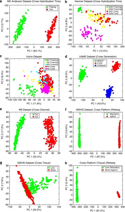
We first applied the principal component analysis to the eight scenarios to visualize the batch (group) effects (Figure 1). Significant batch effects can be seen by the perfect separation of different batches on the PCA score plots for most data sets. For the Hamner, Iconix and NIEHS (cross-tissue) data sets (B, C and G), batch effects exist with overlaps between several batches. Other visualization techniques can also be used to evaluate batch effects such as hierarchical clustering dendrogram, correlation heat-map and variance components pie chart from analysis of variance. The latter is a quantitative technique that gives the variances contributed by all factors when the class labels of all the samples are available. This allows the comparison of variances contributed by batch effects, biological effects and other effects. However, for cross-batch prediction in real applications, the class labels of the samples in the test set (future batch) are to be predicted and are unavailable, and thus analysis of variance cannot be applied for the endpoint factor. This approach is useful for evaluating the sources of variation and process control of sample handling and processing when all of these factors are recorded and reported.

Figure 1.

Score plot of the first two principal components for the eight scenarios. Batches (groups) are indicated by colors. (a) MD Anderson breast cancer data set. (b) Hamner lung carcinogen data set (two batches in training set hybridized in 2005 and 2006, and two batches in test set hybridized in 2007 and 2008). (c) Iconix liver tumor data set (three batches in training set and two in test set). (d) UAMS multiple myeloma data set (the three batches represent three generations of Affymetrix chips on Homo Sapiens). (e) Cologne neuroblastoma data set (the two batches represent the two channels of Agilent arrays). (f) NIEHS data set (cross-platform: the two groups represent Affymetrix and Agilent microarray platforms. For brevity, PCA is performed for common genes with Refseq mapping only. The plots for common genes with Unigene and Sequence mappings are similar). (g) NIEHS data set (cross-tissue: the two groups represent liver and blood samples profiled on Agilent array). (h) NIEHS data set (cross-tissue-and-cross-platform: the two groups represent liver samples profiled on Affymetrix arrays and blood samples profiled on Agilent arrays).

Cross-batch prediction results

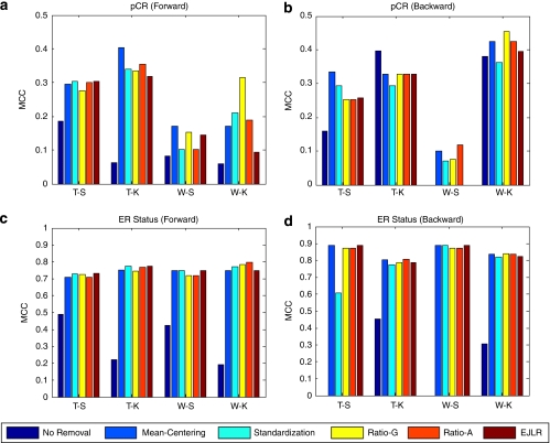
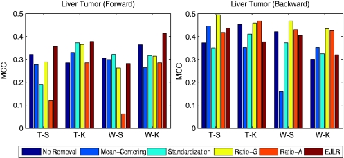
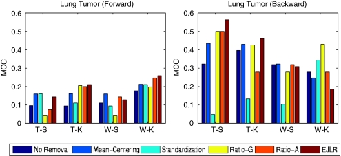
The detailed results for each data set and each endpoint are presented below. The cross-batch prediction performances are shown in Figures 2, 3, 4, 5, 6, 7, 8, 9 and 10 in terms of MCC. It is noteworthy that, for several cases, the predicted values of MCC are zero and thus the corresponding columns are not shown.

Figure 2.

Forward and backward cross-batch prediction performance (y axis) in terms of MCC with different combinations of feature selection and classification algorithm (x axis). (a–b) MD Anderson breast cancer dataset (endpoint: pCR, batch effect cause: different hybridization dates); (c–d) MD Anderson breast cancer data set (endpoint: estrogen receptor status, batch effect cause: different hybridization dates).

Figure 3.

Forward and backward cross-batch prediction performance (y axis) in terms of MCC with different combinations of feature selection and classification algorithm (x axis). Iconix data set (endpoint: liver tumor, batch effect cause: different hybridization dates).

Figure 4.

Forward and backward cross-batch prediction performance (y axis) in terms of MCC with different combinations of feature selection and classification algorithm (x axis). Hamner data set (endpoint: lung tumor, batch effect cause: different hybridization dates).

Figure 5.

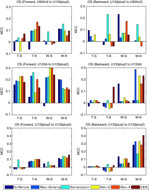
Forward and backward cross-batch prediction performance (y axis) in terms of MCC with different combinations of feature selection and classification algorithm (x axis). UAMS data set (endpoint: OS, batch effect cause: different generations of chips).

Figure 6.

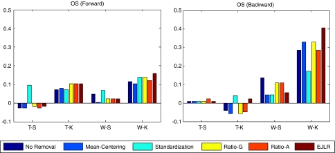
Forward and backward cross-batch prediction performance (y axis) in terms of MCC with different combinations of feature selection and classification algorithm (x axis). Cologne data set, endpoint: OS, batch effect cause: different channels).

Figure 7.

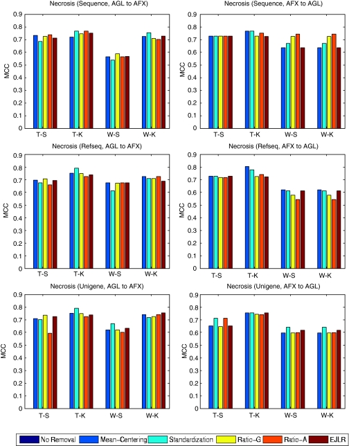
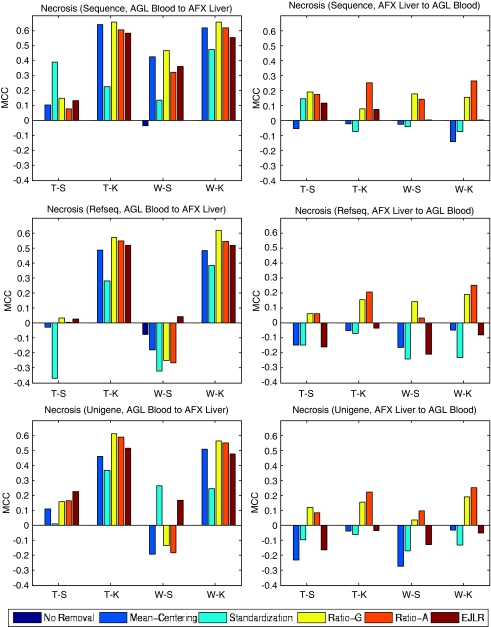
Forward and backward cross-batch prediction performance (y axis) in terms of MCC with different combinations of feature selection and classification algorithm (x axis). NIEHS data set, endpoint: Necrosis, batch effect cause: different microarray platforms).

Figure 8.

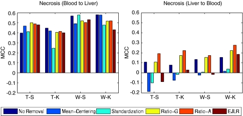
Forward and backward cross-batch prediction performance (y axis) in terms of MCC with different combinations of feature selection and classification algorithm (x axis) (NIEHS data set, endpoint: Necrosis, batch effect cause: different tissues).

Figure 9.

Forward and backward cross-batch prediction performance (y axis) in terms of MCC with different combinations of feature selection and classification algorithm (x axis) (NIEHS data set, endpoint: Necrosis, batch effect cause: Different microarray platforms and different tissues).

Figure 10.

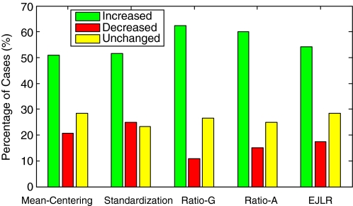
Percentages of increased, decreased and unchanged cases in prediction performance after applying different batch effect removal methods. The total number of cases explored is 120.

Application to the MD Anderson breast cancer data set (pCR and estrogen receptor status)

For the pCR endpoint, both forward and backward predictions indicate improvement or substantial improvement in MCC after batch effect removal for most cases. Backward prediction with T-K combination is the only case where there is a slight decrease in prediction performance (Figures 2a and b). It should be noted that for the T-K combination, the MCC for no removal is very small (∼0.05) in the forward prediction, whereas the largest (∼0.4) in the backward prediction. The reason for this asymmetric performance difference is unclear.

Estrogen receptor status is an endpoint relatively easy to predict. The results show that the cross-batch prediction performances are improved significantly after batch effect removal except the T-S combination for the backward direction. The differences between the performances of different methods are minor (Figures 2c and d).

Application to the iconix data set (liver tumor)

There are three batches in the training set and two batches in the test set (Table 2). Figure 3 shows the prediction performance before and after batch effect removal using the Iconix data set. The top two plots display the performance of forward prediction, from the training set to the test set, and backward prediction, from the test set to the training set. Owing to the increased variability of prediction performance, it is hard to draw a definite conclusion. In general, we see that Ratio-G and the EJLR approaches perform better than or similar to no batch effect removal.

Application to the hamner data set (lung tumor)

There are two batches in the training set and two batches in the test set (Table 3). The same batch effect removal methods were used within the training set and the test set, as well as between these two sets. The performance of the forward prediction is generally worse than that of the backward prediction as seen from the top two plots of Figure 4. Apart from the W-K combination in the backward prediction, mean-centering and EJLR performed better than no batch effect removal.

Application to the UAMS data set (University of Arkansas Medical School, overall survival)

OS is a challenging endpoint to predict, as observed by the MAQC-II.⁵ For the majority of the forward prediction cases, except the W-S combination in the direction from U95Av2 to U133plus2, the T-K combination from U133A to U133plus2, and the W-S combination from U133plus2 to U133plus2, batch effect removal produced better prediction performance than no-removal (Figure 5). However, in the backward predictions, none of these batch effect removal methods appear to yield consistently better prediction results than no-removal. This difficulty may be due to the clinical nature of this endpoint, which is notoriously hard to predict.

Application to the cologne data set (University of Cologne, overall survival)

For the OS endpoint, there is a considerable variation in the prediction performance of different batch effect removal methods (Figure 6).

Application to the NIEHS (Necrosis, cross-platform) data set

Without batch (group) effect removal, all the predictive models fail the predictions completely, noting that the MCC values are zero and no columns are shown for these cases in Figure 7. The application of all batch effect removal methods substantially enhances the prediction performance with any of the three mapping relationships.

Application to the NIEHS (necrosis, cross-tissue) data set

For the forward prediction, from blood to liver, the application of different batch effect removal methods generally does not appear to affect the prediction performance. The backward prediction, from liver to blood, has poor prediction performance with or without the application of batch effect removal algorithms (Figure 8). This may in part be due to the fact that although blood gene signatures can be used to effectively predict liver necrosis, liver gene signatures do not have predictive power for necrosis measured in blood. This finding is consistent with the observations reported by Huang et al.¹⁴

Application to the NIEHS (necrosis, cross-tissue-cross-platform) data set

Without batch (group) effect removal, there is no predictive power either from blood (Agilent) to liver (Affymetrix), or vice versa, noting that all the MCC values are either zero or negative (Figure 9). In using data from blood (Agilent) to predict liver injury (Affymetrix), the applications of most batch effect removal methods enhance the prediction performance except the W-S combination for Refseq and Unigene mapping. When using data from liver (Affymetrix) to predict appropriate blood-based genes (Agilent), the application of batch effect removal methods yields both increased and decreased prediction performance. However, the two ratio-based methods consistently outperform the other methods. Similar to the cross-tissue results, we see that the blood samples have strong predictability of the liver necrosis with proper batch effect removal. However, the predictability is much weaker for backward prediction, from liver to blood. In general, the sequence mapping slightly outperforms the other two mappings.

Meta analysis

To evaluate the general impact of batch effect removal in cross-batch (group) prediction performance, we calculate the increase of prediction performance value MCC after batch effect removal ΔMCC=MCC_After−MCC_Before. If ΔMCC is greater than or lower than a threshold value, we say the batch effect removal has a positive or negative impact on the performance, respectively. If the difference in MCC after and before batch impact removal is less than the threshold, we say the impact is negligible. For simplicity, the threshold is chosen as 0.05.

Figure 10 shows the percentages of cases with increased, decreased and unchanged predictive performances (with sum 100%) over the 120 cases explored. We find that, for each batch effect removal method, the number of cases with increased predictive performance is greater than that with decreased predictive performance, indicating that, in general, batch effect removal has a positive impact on prediction performance. The Ratio-G, Ratio-A, EJLR, mean-centering and standardization methods perform better or equivalent to no batch effect removal in 89, 85, 83, 79 and 75% of the cases, respectively, suggesting that the ratio-based methods are more consistent in positively impacting the prediction performance. We performed the class label bootstrap estimation of the performance differences for a few endpoints and verified that the improvement due to the usage of batch correction methods (data not shown here) was consistent with the simple counting results shown above. Considering the heavy computational cost involved due to the combinatorial nature of the work, we were not able to perform the bootstrap calculation for all endpoints.

Discussion

Batch effects are ubiquitous in microarray experiments. Cross-batch prediction is one of the most important requirements in microarray gene expression analysis, especially in the context of discovering and validating diagnostic, prognostic and predictive gene expression signatures and subsequent biomarker development. This paper systematically evaluated the impact of batch effect removal on cross-batch (group) prediction performance. Five commonly used batch effect removal methods, Ratio-A, Ratio-G, EJLR, mean-centering and standardization, were evaluated using six data sets with eight sources of batch (group) effects and multiple choices of predictive model construction procedures. The total number of cases evaluated is 120. This paper provides and points to a publicly available resource (http://www.fda.gov/nctr/science/centers/toxicoinformatics/maqc/) for future studies on the development and evaluation of batch effects removal algorithms.

The results indicate that the application of all these five methods is generally advisable, and the ratio-based methods are preferred. This preference is also supported by the reasoning that the ratio-based methods are less affected by imbalance of negative/positive sample distributions in different batches. For example, when the future batch has a reverse negative/positive ratio design compared to the training batch, the batch effects and biological effects are confounded and the application of mean-centering and standardization methods may run the risk of distorting biological differences after removing batch effects.

The application of ratio-based methods is straightforward when calibration samples are available for reference. Of the data sets studied, only the Iconix data set provides these samples. We thus recommend, as a good practice and to facilitate further examination, the inclusion of a few (3–5) calibration samples in each batch, for both clinical and toxicogenomics microarray data sets. The availability of these calibration samples may play an important role in the better assessment of existing batch effects, the effectiveness of batch effect removal methods, and the applicability of constructed predictive models to future data sets. It is desirable to have a large sample size or good quality data in each batch, so that the characteristics of each batch can be summarized more accurately and batch effects can be removed more effectively. If the sample sizes of the training and the test set are too small, it is difficult to draw a conclusive inference due to the large uncertainty. In the context of implementing an array-based diagnostic test in a clinical setting, it should be appreciated that batches may, in practice, be composed of a single clinical sample. In this regard, the use of reference samples for the purpose of calibrating batch effects may be of paramount importance.

Significant batch effects exist between ratio-based data and intensity-based data in the cases of cross-platform, cross-platform-and-cross-tissue data sets. Batch effect removal by any of the evaluated methods significantly improves the cross-group prediction performance. The batch effects are strong in the MD Anderson data set. The prediction performances are enhanced after applying batch effect removal methods for both endpoints. When the endpoints are hard to predict such as the cases of Hamner, Iconix and the OS endpoint with the UAMS data set, the application of batch effect removal methods do not necessarily result in a positive impact. The degree of difficulty in the prediction of an endpoint may be evaluated by the predictive performance through internal cross-validation.

It is important to note that the conclusions reached in this study are related to the application of batch effect removal in the context of cross-batch prediction performance with models, which are developed with parametric and non-parametric rank-based feature selection. These methods are intrinsically driven by hypothesis tests that are susceptible to bias introduced by batch effects. Models built with other methods of feature selection including wrapper methods (such as recursive feature elimination) were not evaluated. Wrapper methods select features based on their contribution to model performance during the training process, not through hypothesis-driven tests in an independent step. It is not known explicitly if this process is more or less susceptible to bias than the methods considered in this study and also if the specific conclusions drawn here apply to such model development techniques. Similarly, the other batch effect removal methods as mentioned in the Introduction section also need to be evaluated in future work. Prediction performance metric, AUC has been commonly used in literature and shall be considered for future work. AUC has the advantage of evaluating the performance across the full range of sensitivity and specificity compared with MCC, which is evaluated on one fixed operating point. The current work focuses on cross-batch predictions, which is based on the pre-specified training set and test set. To take full consideration of sample variability, further investigation using randomized split of the training set and test set such as reviewed in Scherer¹⁹ may be performed.

Glossary

DWD

distance-weighted discrimination

EJLR

Extended Johnson-Li-Rabinovic Method

KNN

K-nearest neighbor

MAQC

MicroArray Quality Control Consortium

MAQC-II

MicroArray Quality Control Consortium Phase II

MCC

Matthews Correlation Coefficient

OS

overall survival

PCA

principal component analysis

pCR

pathological complete response

Ratio-A

ratio-based approach (arithmetic mean as reference)

Ratio-G

ratio-based approach (Geometric mean as reference)

SVM

support vector machines

T-S

T test with SVM

T-K

T test with KNN

W-S

Wilcoxon rank sum test with SVM

W-K

Wilcoxon rank sum test with KNN

The authors declare no conflict of interest.

References

- Affymetrix Microarray Suite User GuideVersion 5. Affymetrix2001
- Irizarry RA, Hobbs B, Collin F, Beazer-barclay YD, Antonellis KJ, Scherf U, et al. Exploration, normalization, and summaries of high density oligonucleotide array probe level data. Biostatistics. 2003;4:249–264. doi: 10.1093/biostatistics/4.2.249. [DOI] [PubMed] [Google Scholar]
- Li C, Wing H.DNA-Chip Analyzer (dChip). The analysis of gene expression data: methods and softwareG Parmigiani, ES Garrett, R Irizarry and SL Zeger (eds).Springer, New York; 2003120–141. [Google Scholar]
- Yang Y, Dudoit S, Luu P, Lin DM, Peng V, Ngai J, et al. Normalization for cDNA microarray data: a robust composite method addressing single and multiple slide systematic variation. Nucleic Acids Res. 2002;30:e15. doi: 10.1093/nar/30.4.e15. [DOI] [PMC free article] [PubMed] [Google Scholar]
- Shi L, Campbell G, Jones W, Campagne F, Walker S, Su Z, et al. MAQC-II Project: a comprehensive study of common practices for the development and validation of microarray-based predictive modelsSubmitted toNat Biotechnol 2010 [DOI] [PMC free article] [PubMed]
- Alter O, Brown PO, Bostein D. Singular value decomposition for genome-wide expression data processing and modeling. Proc Natl Acad Sci USA. 2000;97:10101–10106. doi: 10.1073/pnas.97.18.10101. [DOI] [PMC free article] [PubMed] [Google Scholar]
- Benito M, Parker J, Du Q, Wu J, Xiang D, Perou CM, et al. Removal of systematic microarray data biases. Bioinformatics. 2004;20:105–114. doi: 10.1093/bioinformatics/btg385. [DOI] [PubMed] [Google Scholar]
- Bylesjö M, Eriksson D, Sjödin A, Jansson S, Moritz T, Trygg J. Orthogonal projections to latent structures as a strategy for microarray data normalization. BMC Bioinformatics. 2007;8:207. doi: 10.1186/1471-2105-8-207. [DOI] [PMC free article] [PubMed] [Google Scholar]
- Johnson WE, Li C, Rabinovic A. Adjusting batch effects in microarray expression data using empirical Bayes methods. Biostatistics. 2007;8:118–127. doi: 10.1093/biostatistics/kxj037. [DOI] [PubMed] [Google Scholar]
- Hess KR, Anderson K, Symmans WF, Valero V, Ibrahim N, Mejia JA, et al. Pharmacogenomic predictor of sensitivity to preoperative chemotherapy with paclitaxel and fluorouracil, doxorubicin, and cyclophosphamide in breast cancer. J Clin Oncol. 2006;24:4236–4244. doi: 10.1200/JCO.2006.05.6861. [DOI] [PubMed] [Google Scholar]
- Fielden MR, Brennan R, Gollub J. A gene expression biomarker provides early prediction and mechanistic assessment of hepatic tumor induction by nongenotoxic chemicals. Toxicol Sci. 2007;99:90–100. doi: 10.1093/toxsci/kfm156. [DOI] [PubMed] [Google Scholar]
- Thomas R, Pluta L, Yang L, Halsey T. Application of genomic biomarkers to predict increased lung tumor incidence in 2-year rodent cancer bioassays. Toxicol Sci. 2007;97:55–64. doi: 10.1093/toxsci/kfm023. [DOI] [PubMed] [Google Scholar]
- Lobenhofer EK, Auman JT, Blackshear PE, Boorman GA, Bushel PR, Cunningham ML, et al. Gene expression response in target organ and whole blood varies as a function of target organ injury phenotype. Genome Biol. 2008;9:R100. doi: 10.1186/gb-2008-9-6-r100. [DOI] [PMC free article] [PubMed] [Google Scholar]
- Fan X, Lobenhofer E, Chen M, Shi W, Huang J, Luo J, et al. Consistency of predictive signature genes and classifiers generated using different microarray platformsaccepted byPharmocogenomics J 2010 [DOI] [PMC free article] [PubMed]
- Huang J, Shi W, Zhang J, Chou J, Paules R, Gerrish K, et al. Genomic Indicators of Hepatotoxicity conferred through perturbed biological processes and pathways in the bloodaccepted byPharmocogenomics J 2010
- Shaughnessy JD, Jr, Zhan F, Burington BE, Huang Y, Colla S, Hanamura I, et al. A validated gene expression model of high-risk multiple myeloma is defined by deregulated expression of genes mapping to chromosome 1. Blood. 2007;109:2276–2284. doi: 10.1182/blood-2006-07-038430. [DOI] [PubMed] [Google Scholar]
- Oberthuer A, Berthold F, Warnat P, Hero B, Kahlert Y, Spitz R, et al. Customized oligonucleotide microarray gene expression-based classification of neuroblastoma patients outperforms current clinical risk stratification. J Clin Oncol. 2006;24:5070–5078. doi: 10.1200/JCO.2006.06.1879. [DOI] [PubMed] [Google Scholar]
- Walker WL, Liao IH, Gilbert DL, Wong B, Pollard KS, McCulloch CE, et al. Empirical Bayes accommodation of batch-effects in microarray data using identical replicate reference samples: application to RNA expression profiling of blood from Duchenne muscular dystrophy patients. BMC Genomics. 2008;9:494–506. doi: 10.1186/1471-2164-9-494. [DOI] [PMC free article] [PubMed] [Google Scholar]
- Scherer A.Batch Effects and Noise in Microarray Experiments: Sources and Solutions Wiley Series Probability Statistics 2009. 272 pp.