A New and Efficient Poisson-Boltzmann Solver for Interaction of Multiple Proteins

Abstract

We derive a new numerical approach to solving the linearized Poisson Boltzmann equation (PBE) by representing the protein surface as a collection of spheres in which the surface charges can then be iteratively solved by new analytical multipole methods previously introduced by us [Lotan & Head-Gordon, 2006]. We show that our Poisson Boltzmann semi-analytical method, PB-SAM, realizes better accuracy, more flexible memory management, and at reduced cost relative to either finite difference or boundary element method PBE solvers. We provide two new benchmarks of PBE solution accuracy to test the numerical PBE solutions based on (1) arrays of up to hundreds of spherical low dielectric geometries with asymmetric charges in which mutual polarization is treated exactly, and (2) two overlapping spheres with increasing charge asymmetry by solving the PB-SAM method to very high pole order. We illustrate the strength of the PB-SAM approach by computing the potential profile of an array of 60 T1-particle forming monomers of the bromine mosaic virus.

INTRODUCTION

The formation of protein complexes is ubiquitous in a crowded, salty cellular environment. Since electrostatic forces dominate the earliest of protein-protein recognition events in the cell, various analytical and numerical continuum theories of bulk electrolytes have been adapted for use to describe protein complexation mechanisms on the supramolecular scale.² One popular continuum mean-field theory is the Poisson-Boltzmann (PB) treatment, which forms the basis of Gouy-Chapman theory^3,4 in electrochemistry, and under the low field linearized PB (LPB) approximation, the Debye-Hückel theory in solution chemistry⁵ and Derjaguin-Landau-Verwey-Overbeek (DLVO) theory in colloid chemistry^6,7. Numerous techniques for solving the PB equation exist^{1, 6}, including both analytical or numerical methods, and each has its drawbacks and its strengths.

Analytical methods typically allow rapid solution of the PB equation using multipole expansions under specialized geometries such as spheres or cylinders. A complete PB solution comprising one spherical macromolecule was developed by Kirkwood⁸ more than 70 years ago, but generalization of this complete solution to two or more spherical macromolecules proved to be more difficult, and many different partial and approximate solutions have been proposed^9–12. We have recently achieved a fundamental result in deriving an analytical PB solution for computing the screened electrostatic interaction between arbitrary numbers of spherical proteins of arbitrarily complex charge distributions, separated by arbitrary distance¹. While such idealized protein geometries will typically be inappropriate for describing complexation on a supermolecular scale, this new analytical solution is a novel component of our new numerical PB solver for arbitrary protein shape. It also serves as a benchmark for the accuracy of the numerical solutions in certain idealized test cases.

By contrast, numerical methods (see reference [13] for a recent survey) such as finite-difference (FD)^14–19 and finite-element (FE)^20–22 methods can handle arbitrary dielectric boundaries by solving for the PB potential on a 3-D grid or mesh. However there are limitations of the FE or FD formulations, such as singularities in the potential solution due to point charges, that electric displacement continuity could not be enforced across dielectric boundaries (thereby reducing the solution accuracy and convergence rate), and forces must be estimated from finite-difference calculations.¹³ But most importantly, the requirement that the solution be solved on a grid limits its practical application to spatial domains of either two to three typical macromolecules at reasonably high resolution (~0.2Å), or to larger numbers of macromolecules with greatly diminished resolution and thus solution accuracy. For example, the PBE solution for an assembled 50S ribosomal subunit has been evaluated at 0.45Å resolution¹⁴, at the limit of machine memory, but to describe the preceding assembly process that occur over much larger spatial distances, the spatial resolution and consequently the solution accuracy would greatly deteriorate. As such, computational and memory cost in FD and FE methods are strictly functions of the number of grid points, and not the number of macromolecules described.

Boundary element (BE) methods^22–29 are an attractive alternative since they satisfy both the Dirichlet and von Neuman boundary conditions by construction, singular charges can be correctly treated, and most importantly the 2D solutions on the macromolecular surface removes spatial resolution limitations imposed by the 3D grid of the FD or FE solvers. However increasing the number of boundary surface element results in an increasingly large dense matrix to be solved with severe memory requirements, a problem which scales with the number of macromolecules. Recent acceleration of the BE approach^24,26 by incorporating fast multipole methods have rendered BE computational times comparable to state-of-the-art software packages like the Adaptive Poisson Boltzmann Solver (APBS)¹⁴ based on FD solutions.

In this work we derive a new numerical approach to solving the PB equation by combining the advantages of both the boundary element and our analytical model¹ formalism. In particular, we replace the discretization of the molecule surface into a large number (tens of thousands) of boundary elements, by a discretization involving a smaller number (tens to hundreds) of spheres. The surface charges can then be iteratively solved using analytical multipole methods¹. We show that our Poisson Boltzmann semi-analytical method, PB-SAM, converges to the analytical solution with better accuracy and at greatly reduced cost relative to the readily available public domain PB solver APBS.¹⁴ Furthermore, we define a high quality benchmark using 140 poles to describe the electrostatic potential for two overlapping spheres that are models for the sharp features that are sometimes present in real protein geometries, in which we show that our PB-SAM solution converges to the correct solution with the same computational cost or better than the finite difference solution. Finally we illustrate the strength of the PB-SAM approach by computing the potential profile of an array of 60 T1-particle forming monomers of the bromine mosaic virus (PDB code 1YC6).

THEORY

Mathematical Preliminaries

Our theory makes extensive use of the spherical harmonics (SH) family of functions. The spherical harmonic function of order n and degree m, at polar angle θ and azimuthal angle φ, is defined per the convention from Gumerov and Duraiswami³⁰ as

$$Y_{nm}(\theta ,\phi )={(-1)}^m\sqrt{\frac{(n-\mid m\mid )!}{(n+\mid m\mid )!}}{P}_{n\mid m\mid }(cos\theta )e^{im\phi }$$ (1)

where P_nm (x) is the associated Legendre polynomial. Note that this definition of Y_nm(θ,φ) differs from the common convention by a $\sqrt{(2n+1)/4\pi }$ factor. The complex conjugate of Y_nm(θ,φ) will be denoted as $\overline{Y_{nm}}(\theta ,\phi )$.

We shall utilize two important properties of spherical harmonics – their addition theorems and orthogonality. Let r₁ = [r₁,θ₁,φ₁] and r₂ = [r₂,θ₂,φ₂] be two points in 3D space specified by spherical coordinates, where r₂ > r₁. The Euclidean distance |r₁−r₂| between them then obeys the addition theorems^24,31:

$$\frac{1}{\mid {\mathbf{r}}_{\mathbf{1}}-{\mathbf{r}}_{\mathbf{2}}\mid }=\sum _{n=0}^{\infty }\sum _{m=-n}^n\frac{r_1^n}{r_2^{n+1}}\overline{Y_{nm}}({\theta }_1,{\phi }_1)Y_{nm}({\theta }_2,{\phi }_2)$$ (2a)

and for the screened Yukawa potential Eq. (2a) is modified to read as

$$\frac{e^{-\kappa \mid {\mathbf{r}}_{\mathbf{1}}-{\mathbf{r}}_{\mathbf{2}}\mid }}{\mid {\mathbf{r}}_{\mathbf{1}}-{\mathbf{r}}_{\mathbf{2}}\mid }=\sum _{n=0}^{\infty }\sum _{m=-n}^n\frac{r_1^n}{r_2^{n+1}}{\widehat{i}}_n(\kappa r_1)e^{-\kappa r_2}{\widehat{k}}_n(\kappa r_2)\overline{Y_{nm}}({\theta }_1,{\phi }_1)Y_{nm}({\theta }_2,{\phi }_2)$$ (2b)

where κ is the inverse Debye Huckel screening length (described later), and k̂_n(z) and î_n(z) are adapted modified spherical Bessel functions defined as

$${\widehat{k}}_n(z)=\sqrt{\frac{2}{\pi }}\frac{e^z{z}^{n+1/2}}{(2n-1)!!}{K}_{n+1/2}(z)$$ (3a)

$${\widehat{i}}_n(z)=\sqrt{\frac{\pi }{2}}\frac{(2n+1)!!}{z^{n+1/2}}{I}_{n+1/2}(z)$$ (3b)

I_n(z) and K_n(z) are the modified Bessel functions of the first and second kind respectively. Detailed properties of k̂_n(z) and î_n(z) have been described in ref 1.

The spherical harmonic functions are also orthogonal over the surface of a unit sphere (S₁):

$${\int }_{\phi =0}^{2\pi }{\int }_{\theta =0}^{\pi }{Y}_{ls}(\theta ,\phi )\overline{Y_{nm}}(\theta ,\phi )sin\theta \partial \theta \partial \phi =\frac{4\pi }{2n+1}{\delta }_{nl}{\delta }_{ms}$$ (4a)

Hence a square-integrable function g(θ,φ) on S₁ can be expanded using {Y_nm} as the basis set:

$$g(\theta ,\phi )=\sum _{n=0}^{\infty }\sum _{m=-n}^n\frac{2n+1}{4\pi }{G}_{nm}{Y}_{nm}(\theta ,\phi )$$ (4b)

with the coefficients G_nm determined through the reciprocal transform

$$G_{nm}={\int }_{\phi =0}^{2\pi }{\int }_{\theta =0}^{\pi }g({\theta }^{\prime },{\phi }^{\prime })\overline{Y_{nm}}({\theta }^{\prime },{\phi }^{\prime })sin{\theta }^{\prime }\partial {\theta }^{\prime }\partial {\phi }^{\prime }$$ (4c)

Setting up the boundary value problem

We seek to set up a boundary value problem for a system of N_mol macromolecules immersed in an implicit aqueous salty solvent. Figure 1 gives an example of the spatial domain for which we solve the linearized PB equation (LPBE). Each macromolecule I is embedded with $N_C^{(I)}$ fixed partial charge and represented as a collection of $N_S^{(I)}$ overlapping spheres with dielectric constant ε_in. For simplicity we consider in this paper the same ε_in for all molecules, but the model can handle different dielectric constants. The solvent is treated as a continuum with dielectric constant ε_out, with screening effects due to mobile ions captured via the inverse Debye length κ. The LPBE gives the potential Φ at any point r in space ℜ³ as

Figure 1. Setting up the boundary value problem.

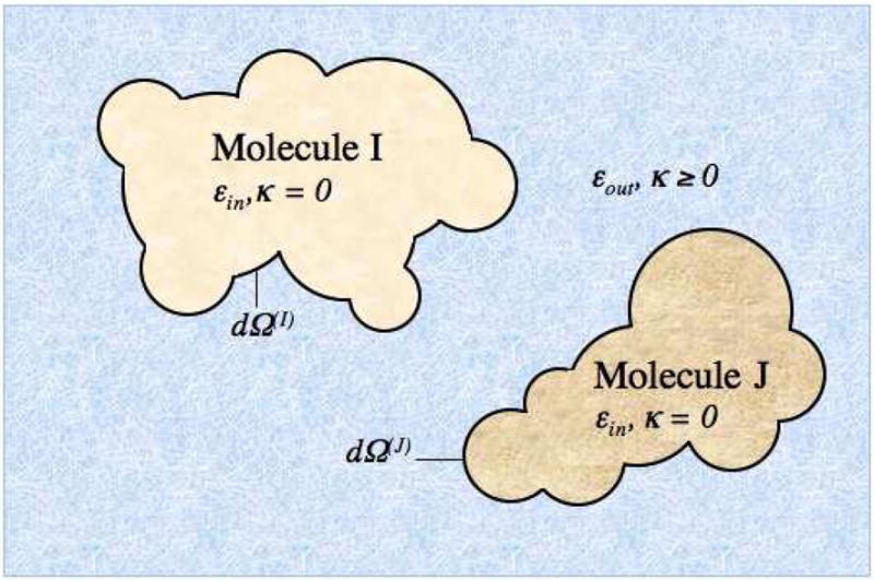
The example system is comprised of two proteins with arbitrary charge distribution, each represented as a collection of overlapping spheres to describe an arbitrarily shaped dielectric boundary containing no salt, immersed in a high dielectric salty continuum solvent. Salt screening effects are captured via the Debye Huckel parameter κ.

$$-\nabla [\epsilon (\mathbf{r})\nabla \mathrm{\Phi }(\mathbf{r})]+{\kappa }^2\mathrm{\Phi }(\mathbf{r})=4\pi {\rho }_{\mathit{fixed}}(\mathbf{r})$$ (5)

where ε is the relative dielectric function, ρ_fixed is the charge density due to the fixed protein partial charges, and $\kappa =\sqrt{8\pi \overline{n}{e}^2/{\epsilon }_{\mathit{out}}{k}_{B}T}$, where n̄ is the bulk concentration of monovalent salt in the solution, e is the fundamental electronic charge, k_B the Boltzmann constant, and T the absolute temperature. Inside each macromolecule I, the potential ${\mathrm{\Phi }}_{in}^{(I)}(\mathbf{r})$ satisfies the Poisson equation

$$-{\nabla }^2{\mathrm{\Phi }}_{in}^{(I)}(\mathbf{r})={\rho }_{\mathit{fixed}}^{(I)}(\mathbf{r})/{\epsilon }_{in}$$ (6a)

while in the region outside all macromolecules, the potential Φ_out(r) satisfies the Helmholtz equation

$${\nabla }^2{\mathrm{\Phi }}_{\mathit{out}}(r)-{\kappa }^2{\mathrm{\Phi }}_{\mathit{out}}(r)=0$$ (6b)

We first express the potential ${\mathrm{\Phi }}_{in}^{(I)}(\mathbf{r})$ anywhere inside molecule I as the sum of the potentials due to the embedded fixed charges and a single-layer of yet unknown reaction charges f^(I)(r) on the surface dΩ^{(I) 23,32}

$${\mathrm{\Phi }}_{in}^{(I)}(\mathbf{r})=\sum _{\alpha =1}^{N_C^{(I)}}\frac{1}{\mid \mathbf{r}-{\mathbf{r}}_{\alpha }^{(i)}\mid }\frac{q_{\alpha }^{(I)}}{{\epsilon }_{in}}+\frac{1}{4\pi }\underset{d{\mathrm{\Omega }}^{(I)}}{\int }\frac{1}{\mid \mathbf{r}-{\mathbf{r}}^{\prime }\mid }{f}^{(I)}({\mathbf{r}}^{\prime })d{\mathbf{r}}^{\prime }$$ (7)

In our new approach, the surface of molecule I is discretized into $N_S^{(I)}$ spheres. We consider each sphere k of molecule I of radius a^(I,k) in turn, and all position vectors and coefficients are defined with the center of sphere k as the origin. We apply the first addition theorem (Eq. (2a)) to Eq. (7) to obtain

$${\mathrm{\Phi }}_{in}^{(I,k)}(\mathit{r})=\sum _{n=0}^{\infty }\sum _{m=-n}^n\left(\frac{E_{nm}^{(I,k)}}{r}{\left(\frac{a^{(I,k)}}{r}\right)}^n+{\left(\frac{r}{a^{(I,k)}}\right)}^n{LE}_{nm}^{(I,k)}\right)Y_{nm}^{(I,k)}(\theta ,\phi )+\sum _{n=0}^{\infty }\sum _{m=-n}^n\left({\left(\frac{r}{a^{(I,k)}}\right)}^n({LF}_{nm}^{(I,k)}+{\mathit{LFS}}_{nm}^{(I,k)})\right)Y_{nm}^{(I,k)}(\theta ,\phi )$$ (8)

with the coefficients defined as

$$E_{nm}^{(I,k)}\equiv \sum _{\alpha =1}^{N_C^{(I,k)}}\frac{q_{\alpha }}{{\epsilon }_{in}}{\left(\frac{r_{\alpha }}{a^{(I,k)}}\right)}^n\overline{Y_{nm}^{(I,k)}}({\theta }_{\alpha },{\phi }_{\alpha })$$ (8a)

$${LE}_{nm}^{(I,k)}\equiv \sum _{\alpha =1}^{{\overline{N}}_C^{(I,k)}}\frac{q_{\alpha }}{{\epsilon }_{in}}\frac{1}{r_{\alpha }}{\left(\frac{a^{(I,k)}}{r_{\alpha }}\right)}^n\overline{Y_{nm}^{(I,k)}}({\theta }_{\alpha },{\phi }_{\alpha })$$ (8b)

$${LF}_{nm}^{(I,k)}\equiv \frac{1}{4\pi }\underset{{\overline{d\mathrm{\Omega }}}^{(I,k)}}{\int }\frac{f^{(I,k)}({\mathbf{r}}^{\prime })}{r^{\prime }}{\left(\frac{a^{(I,k)}}{r^{\prime }}\right)}^n\overline{Y_{nm}^{(I,k)}}({\theta }^{\prime },{\phi }^{\prime })d{\mathbf{r}}^{\prime }$$ (8c)

$${\mathit{LFS}}_{nm}^{(I,k)}\equiv \frac{1}{4\pi }\underset{d{\mathrm{\Omega }}^{(I,k)}}{\int }\frac{f^{(I,k)}({\mathbf{r}}^{\prime })}{r^{\prime }}{\left(\frac{a^{(I,k)}}{r^{\prime }}\right)}^n\overline{Y_{nm}^{(I,k)}}({\theta }^{\prime },{\phi }^{\prime })d{\mathbf{r}}^{\prime }$$ (8d)

Notice that we have scaled the terms with $r_{\alpha }^n$ and $r_{\alpha }^{n+1}$ dependence by (a^(I,k))ⁿ and (a^(I,k))⁻ⁿ respectively. This is to avoid machine imprecision as n becomes large. Coefficients with (r_α/a^(I,k))ⁿ dependence, such as $E_{nm}^{(I,k)}$, are known as multipole (external) coefficients, while those with a^(I,k)n/r_α^{n +1} dependence ( ${LE}_{nm}^{(I,k)},{LF}_{nm}^{(I,k)}$ and ${\mathit{LFS}}_{nm}^{(I,k)}$) are known as Taylor (local) coefficients. The first sum in Eq. (8) represents the potential due to fixed charges, where $E_{nm}^{(i,k)}$ sums over $N_C^{(I,k)}$ fixed charges inside sphere k of molecule I, while ${LE}_{nm}^{(I,k)}$ sums over the remaining ${\overline{N}}_C^{(I,k)}$ fixed charges outside sphere k. The second sum in Eq. (8) gives the potential due to the unknown surface charge f^(I)(r); ${\mathit{LFS}}_{nm}^{(I,k)}$ and ${LF}_{nm}^{(I,k)}$ account for represents reactive charges on sphere k, and on other spheres in molecule I, respectively.

In the solvent region outside the molecules, the potential Φ_out(r) can be represented as the sum of Yukawa potentials due to each molecule’s yet unknown effective surface charges h^(I)(r)^23,32

$${\mathrm{\Phi }}_{\mathit{out}}(\mathbf{r})=\sum _{I=1}^{N_{\mathit{mol}}}\left(\frac{1}{4\pi }\underset{d{\mathrm{\Omega }}^{(I)}}{\int }\frac{e^{-\kappa \mid \mathbf{r}-{\mathbf{r}}^{\prime }\mid }}{\mid \mathbf{r}-{\mathbf{r}}^{\prime }\mid }{h}^{(I)}({\mathbf{r}}^{\prime })d{\mathbf{r}}^{\prime }\right)$$ (9)

The above equation valid for the exposed portion of sphere k of molecule I. Applying addition theorem 2 (Eq. (2b)) to Eq. (9), the potential on the exposed surface can be expressed as

$${\mathrm{\Phi }}_{\mathit{out}}^{(I,k)}(\mathbf{r})=\sum _{n=0}^{\infty }\sum _{m=-n}^n\left(\frac{H_{nm}^{(I,k)}}{r}{\left(\frac{a^{(I,k)}}{r}\right)}^n{e}^{-\kappa r}{\widehat{k}}_n(\kappa r)+{\left(\frac{r}{a^{(I,k)}}\right)}^n{\widehat{i}}_n(\kappa r)({LH}_{nm}^{(I,k)}+LH{N}_{nm}^{(I,k)})\right)Y_{nm}^{(I,k)}(\theta ,\phi )$$ (10)

where the coefficients are defined as

$$H_{nm}^{(I,k)}\equiv \frac{1}{4\pi }\underset{d{\mathrm{\Omega }}^{(i,k)}}{\int }{h}^{(I,k)}({\mathbf{r}}^{\prime }){\left(\frac{r^{\prime }}{a^{(I,k)}}\right)}^n{\widehat{i}}_n(\kappa r^{\prime })\overline{Y_{nm}^{(I,k)}}({\theta }^{\prime },{\phi }^{\prime })d{\mathbf{r}}^{\prime }$$ (10a)

$${LH}_{nm}^{(I,k)}\equiv \frac{1}{4\pi }\underset{d{\overline{\mathrm{\Omega }}}^{(I,k)}}{\int }\frac{h^{(I,k)}({\mathbf{r}}^{\prime })}{r^{\prime }}{\left(\frac{a^{(I,k)}}{r^{\prime }}\right)}^n{e}^{-\kappa r^{\prime }}{\widehat{k}}_n(\kappa r^{\prime })\overline{Y_{nm}^{(I,k)}}({\theta }^{\prime },{\phi }^{\prime })d{\mathbf{r}}^{\prime }$$ (10b)

$$LH{N}_{nm}^{(I,k)}\equiv \sum _{J\ne I}^{N_{\mathit{mol}}}\sum _{l=1}^{N_S^{(J)}}\left(\frac{1}{4\pi }\underset{d{\mathrm{\Omega }}^{(J,l)}}{\int }\frac{h^{(J,l)}({\mathbf{r}}^{\prime })}{r^{\prime }}{\left(\frac{a^{(I,k)}}{r^{\prime }}\right)}^n{e}^{-\kappa r^{\prime }}{\widehat{k}}_n(\kappa r^{\prime })\overline{Y_{nm}^{(I,k)}}({\theta }^{\prime },{\phi }^{\prime })d{\mathbf{r}}^{\prime }\right)$$ (10c)

The multipole coefficient $H_{nm}^{(I,k)}$ represents effective polarization charges on sphere k of molecule I’s exposed surface. The local coefficients ${LH}_{nm}^{(I,k)}$ and $LH{N}_{nm}^{(I,k)}$ represent effective polarization charges on other spheres in molecule I, and on other molecules, respectively.

With equations (8) and (10) in hand, we can impose boundary conditions at the dielectric boundary surface ${\mathbf{r}}_E=(a^{(I,k)},{\theta }_E,{\phi }_E)\in d{\mathrm{\Omega }}_E^{(I,k)}$ between each sphere k in molecule I exposed to solvent:

$${\mathrm{\Phi }}_{in}^{(I,k)}({\mathbf{r}}_E)={\mathrm{\Phi }}_{\mathit{out}}^{(I,k)}({\mathbf{r}}_E)$$ (11a)

$${\epsilon \frac{d{\mathrm{\Phi }}_{in}^{(I,k)}}{dn}|}_{{\mathbf{r}}_E}={\frac{d{\mathrm{\Phi }}_{\mathit{out}}^{(I,k)}}{dn}|}_{{\mathbf{r}}_E},\epsilon ={\epsilon }_{in}/{\epsilon }_{\mathit{out}}$$ (11b)

The Dirichlet boundary condition (Eq. 11a) enforces potential continuity across the boundary

$$\sum _{n=0}^{\infty }\sum _{m=-n}^n(E_{nm}^{(I,k)}+a^{(I,k)}({LE}_{nm}^{(I,k)}+{LF}_{nm}^{(I,k)}+{\mathit{LFS}}_{nm}^{(I,k)}))Y_{nm}^{(I,k)}({\theta }_E,{\phi }_E)=\sum _{n=0}^{\infty }\sum _{m=-n}^n(H_{nm}^{(I,k)}{e}^{-\kappa a^{(I,k)}}{\widehat{k}}_n(\kappa a^{(I,k)})+a^{(I,k)}{\widehat{i}}_n(\kappa a^{(I,k)})({LH}_{nm}^{(I,k)}+LH{N}_{nm}^{(I,k)}))Y_{nm}^{(I,k)}({\theta }_E,{\phi }_E)$$ (12a)

while the von Neumann boundary condition (Eq. 11b) enforces electric displacement continuity

$$\epsilon \sum _{n=0}^{\infty }\sum _{m=-n}^n\left(-(n+1)E_{nm}^{(I,k)}+n{F}_{nm}^{(I,k)}+n{a}^{(I,k)}({LE}_{nm}^{(I,k)}+{LF}_{nm}^{(I,k)})\right)Y_{nm}^{(I,k)}({\theta }_E,{\phi }_E)=\sum _{n=0}^{\infty }\sum _{m=-n}^n\left(H_{nm}^{(I,k)}{e}^{-\kappa a^{(I,k)}}\left[n{\widehat{k}}_n(\kappa a^{(I,k)})-(2n+1){\widehat{k}}_{n+1}(\kappa a^{(I,k)})\right]+a^{(I,k)}\left[n{\widehat{i}}_n(\kappa a^{(I,k)})+\frac{{(\kappa a^{(I,k)})}^2{\widehat{i}}_{n+1}(\kappa a^{(I,k)})}{2n+3}\right]({LH}_{nm}^{(I,k)}+LH{N}_{nm}^{(I,k)})\right)Y_{nm}^{(I,k)}({\theta }_E,{\phi }_E)$$ (12b)

We have introduced $F_{nm}^{(I,k)}\equiv a^{(I,k)}{\mathit{LFS}}_{nm}^{(I,k)}$. We continue to simplify Eqs. (12a) and (12b) by rearranging

$$\sum _{n=0}^{\infty }\sum _{m=-n}^n(-H_{nm}^{(I,k)}{e}^{-\kappa u^{(I,k)}}{\widehat{k}}_n(\kappa a^{(I,k)})+F_{nm}^{(I,k)}+X{H}_{nm}^{(I,k)})Y_{nm}^{(I,k)}({\theta }_E,{\phi }_E)=0$$ (13a)

$$\sum _{n=0}^{\infty }\sum _{m=-n}^n\left(e^{-\kappa a^{(I,k)}}\left[n{\widehat{k}}_n(\kappa a^{(I,k)})-(2n+1){\widehat{k}}_{n+1}(\kappa a^{(I,k)})\right]H_{nm}^{(I,k)}-n\epsilon F_{nm}^{(I,k)}+X{F}_{nm}^{(I,k)}\right)Y_{nm}^{(I,k)}({\theta }_E,{\phi }_E)=0$$ (13b)

where

$$X{H}_{nm}^{(I,k)}\equiv E_{nm}^{(I,k)}+a^{(I,k)}({LE}_{nm}^{(I,k)}+{LF}_{nm}^{(I,k)})-a^{(I,k)}{\widehat{i}}_n({ka}^{(I,k)})({LH}_{nm}^{(I,k)}+LH{N}_{nm}^{(I,k)})$$ (14a)

$$X{F}_{nm}^{(I,k)}\equiv a^{(I,k)}\left[n{\widehat{i}}_n({ka}^{(I,k)})+\frac{{(\kappa a^{(I,k)})}^2{\widehat{i}}_{n+1}({ka}^{(I,k)})}{2n+3}\right]({LH}_{nm}^{(I,k)}+LH{N}_{nm}^{(I,k)})+(n+1)\epsilon E_{nm}^{(I,k)}-n\epsilon a^{(I,k)}({LE}_{nm}^{(I,k)}+{LF}_{nm}^{(I,k)})$$ (14b)

The boundary equations above are valid on the solvent-exposed surfaces of sphere k on molecule I. We need another set of boundary equations on the buried surface ${\mathbf{r}}_B=\left[a^{(I,k)},{\theta }_B,{\phi }_B\right]\in d{\mathrm{\Omega }}_B^{(I,k)}$. We shall utilize the fact that there is no polarization charge on the buried surface, i.e. f^(I,k)(r_B) = h^(I,k)(r_B) = 0, since there is no dielectric discontinuity. It follows that scaled versions of the charge distributions, f̃^(I,k)(θ,φ) ≡ (a^(I,k))² f^(I,k)(a^(I,k),θ,φ) and h̃^(I,k)(θ,φ) ≡ (a^(I,k))² h^(I,k)(a^(I,k),θ,φ), are also zero on the buried surface. Separately, we can express f̃^(I,k) and h̃^(I,k) in terms of $F_{nm}^{(I,k)}$ and $H_{nm}^{(I,k)}$ using Eqs. (4c), (8d) and (10a),

$${\stackrel{\sim }{f}}^{(I,k)}(\theta ,\phi )=\sum _{n=0}^{\infty }\sum _{m=-n}^n\frac{2n+1}{4\pi }{F}_{nm}^{(I,k)}{Y}_{nm}^{(I,k)}(\theta ,\phi )$$ (15a)

$${\stackrel{\sim }{h}}^{(I,k)}(\theta ,\phi )=\sum _{n=0}^{\infty }\sum _{m=-n}^n\frac{2n+1}{4\pi }\frac{H_{nm}^{(I,k)}}{{\widehat{i}}_n(\kappa a^{(I,k)})}{Y}_{nm}^{(I,k)}(\theta ,\phi )$$ (15b)

so the ‘zero-charge’ requirement at the buried boundary can be imposed as

$$\sum _{n=0}^{\infty }\sum _{m=-n}^n\frac{2n+1}{4\pi }{F}_{nm}^{(I,k)}{Y}_{nm}^{(I,k)}({\theta }_B,{\phi }_B)=0$$ (16a)

$$\sum _{n=0}^{\infty }\sum _{m=-n}^n\frac{2n+1}{4\pi }\frac{H_{nm}^{(I,k)}}{{\widehat{i}}_n(\kappa a^{(I,k)})}{Y}_{nm}^{(I,k)}({\theta }_B,{\phi }_B)=0$$ (16b)

Equations (13a), (13b), (16a) and (16b) specified the complete boundary value problem, from which $F_{nm}^{(I,k)}$ and $H_{nm}^{(I,k)}$ can be solved.

Solution of the boundary value coefficients and interaction energy

To solve for $F_{nm}^{(i,k)}$ and $H_{nm}^{(i,k)}$, we need to cast the boundary value problem as a linear system of equations. The infinite expansion series must first be truncated at a maximum pole order p, chosen depending on the desired level of accuracy versus computational cost (see Results). The obvious approach is to set up the boundary equations as a linear least square problem (Figure 2a), by discretizing sphere k into M_B buried and M_E exposed grid points, and then finding solutions of vectors F^(I,k)and H^{(I,k )} that best satisfy the appropriate boundary equations on all grid points. Using the DGELSY routine (complete orthogonal factorization) in LAPACK for (M_E + M_B)= 10,000 and p = 60, each sphere is solved in approximately 10 minutes. This is computationally intractable if the LPBE needs to be solved repeatedly for tens to hundreds of spheres during dynamics simulations.

Figure 2. Setting up the boundary equation (Eqns. 13a–b, 16a–b).

(a) As a Linear Least Square solve problem. (b) As a matrix-vector multiply operation.

Instead, we formulated a novel approach that makes use of spherical harmonics’ orthogonal property (Eq. 4). It converts the problem to a direct matrix-vector multiply operation (Figure 2b), which can be evaluated two-orders of magnitude faster than the LLS approach. We first add ${\displaystyle \sum _{n=0}^{\infty }}{\displaystyle \sum _{m=-n}^n}(2n+1)\frac{H_{nm}^{(I,k)}}{{\widehat{i}}_n(\kappa a^{(I,k)})}{Y}_{nm}^{(I,k)}({\theta }_E,{\phi }_E)$ to both sides of Eq. (13a) and divide by 4π to arrive at:

$$\sum _{n=0}^{\infty }\sum _{m=-n}^n\frac{2n+1}{4\pi }\frac{H_{nm}^{(I,k)}}{{\widehat{i}}_n(\kappa a_{ki})}{Y}_{nm}^{(I,k)}({\theta }_E,{\phi }_E)={\stackrel{\sim }{w}}_{H,\mathit{exposed}}({\theta }_E,{\phi }_E)$$ (17a)

where

$${\stackrel{\sim }{w}}_{H,\mathit{exposed}}(\theta ,\phi )=\frac{1}{4\pi }\sum _{n=0}^{\infty }\sum _{m=-n}^n\left(H_{nm}^{(I,k)}\left(\frac{2n+1}{{\widehat{i}}_n(\kappa a^{(I,k)})}-e^{\kappa a^{(I,k)}}{\widehat{k}}_n(\kappa a^{(I,k)})\right)+F_{nm}^{(I,k)}+X{H}_{nm}^{(I,k)}\right)Y_{nm}^{(I,k)}(\theta ,\phi )$$ (17b)

Similarly, we add ${\displaystyle \sum _{n=0}^{\infty }}{\displaystyle \sum _{m=-n}^n}(2n+1)F_{nm}^{(I,k)}{Y}_{nm}^{(I,k)}({\theta }_E,{\phi }_E)$ to both sides of Eq. (13b) and then divide by 4π:

$$\sum _{n=0}^{\infty }\sum _{m=-n}^n\frac{2n+1}{4\pi }{F}_{nm}^{(I,k)}{Y}_{nm}^{(I,k)}({\theta }_E,{\phi }_E)={\stackrel{\sim }{w}}_{F,\mathit{exposed}}({\theta }_E,{\phi }_E)$$ (18a)

$${\stackrel{\sim }{w}}_{F,\mathit{exposed}}(\theta ,\phi )=\frac{1}{4\pi }\sum _{n=0}^{\infty }\sum _{m=-n}^n\left(e^{-{ka}^{(I,k)}}\left[n{\widehat{k}}_n({ka}^{(I,k)})-(2n+1){\widehat{k}}_{n+1}({ka}^{(I,k)})\right]H_{nm}^{(I,k)}+(2n+1-n\epsilon )F_{nm}^{(I,k)}+X{F}_{nm}^{(I,k)}\right)Y_{nm}^{(I,k)}(\theta ,\phi )$$ (18b)

Equations (17a) and (17b) (and similarly (18a) and (18b)) now completely describe functions w̃_H(θ, φ) (and w̃_F(θ, φ) over the entire surface of sphere k:

$$\sum _{n=0}^{\infty }\sum _{m=-n}^n\frac{2n+1}{4\pi }\left[\frac{H_{nm}^{(\text{I},\text{k})}}{{\widehat{i}}_n(\kappa a^{(\text{I},\text{k})})}\right]Y_{nm}^{(\text{I},\text{k})}(\theta ,\phi )={\stackrel{\sim }{w}}_H(\theta ,\phi )=\{\begin{array}{ll}{\stackrel{\sim }{w}}_{H,\mathit{exposed}}(\theta ,\phi ),\hfill & (\theta ,\phi )\in \{{\theta }_E,{\phi }_E\}\hfill \\ 0,\hfill & (\theta ,\phi )\in \{{\theta }_B,{\phi }_B\}\hfill \end{array}$$ (19a)

$$\sum _{n=0}^{\infty }\sum _{m=-n}^n\frac{2n+1}{4\pi }\left[F_{nm}^{(I,k)}\right]Y_{nm}^{(I,k)}(\theta ,\phi )={\stackrel{\sim }{w}}_F(\theta ,\phi )=\{\begin{array}{ll}{\stackrel{\sim }{w}}_{F,\mathit{exposed}}(\theta ,\phi ),\hfill & (\theta ,\phi )\in \{{\theta }_E,{\phi }_E\}\hfill \\ 0,\hfill & (\theta ,\phi )\in \{{\theta }_B,{\phi }_B\}\hfill \end{array}$$ (19b)

The above equations now have the familiar form of spherical harmonic expansion of Eq. (4b), so we can directly evaluate the coefficients in square parentheses via the reciprocal transform Eq. (4c). We show below the derivation for H^(I,k)

$$\begin{array}{l}\frac{H_{nm}^{(I,k)}}{{\widehat{i}}_n(\kappa a^{(I,k)})}={\int }_{\phi =0}^{2\pi }{\int }_{\theta =0}^{\pi }{\stackrel{\sim }{w}}_H({\theta }^{\prime },{\phi }^{\prime })\overline{Y_{nm}^{(I,k)}}({\theta }^{\prime },{\phi }^{\prime })\mathit{sin}{\theta }^{\prime }d{\theta }^{\prime }d{\phi }^{\prime }={\int }_{{\phi }_E}{\int }_{{\theta }_E}{\stackrel{\sim }{w}}_{H,\mathit{exposed}}({\theta }^{\prime },{\phi }^{\prime })\overline{Y_{nm}^{(I,k)}}({\theta }^{\prime },{\phi }^{\prime })\mathit{sin}{\theta }^{\prime }d{\theta }^{\prime }d{\phi }^{\prime }\\ ={\int }_{{\phi }_E}{\int }_{{\theta }_E}\left\{\sum _{l=0}^{\infty }\sum _{s=-l}^l\left(H_{ls}^{(I,k)}\left(\frac{2l+1}{{\widehat{i}}_l(\kappa a^{(i,k)})}-e^{-\kappa a^{(I,k)}}{\widehat{k}}_l(\kappa a^{(I,k)})\right)+F_{ls}^{(I,k)}+X{H}_{ls}^{(I,k)}\right)Y_{ls}^{(I,k)}({\theta }^{\prime },{\phi }^{\prime })\right\}\overline{Y_{nm}^{(I,k)}}({\theta }^{\prime },{\phi }^{\prime })\mathit{sin}{\theta }^{\prime }d{\theta }^{\prime }d{\phi }^{\prime }\\ =\sum _{l=0}^{\infty }\sum _{s=-l}^l{I}_{E,\mathit{lsnm}}^{(I,k)}\left(H_{ls}^{(I,k)}\left(\frac{2l+1}{{\widehat{i}}_l(\kappa a^{(i,k)})}-e^{-\kappa a^{(I,k)}}{\widehat{k}}_l(\kappa a^{(I,k)})\right)+F_{ls}^{(I,k)}+X{H}_{ls}^{(I,k)}\right)\end{array}$$ (20)

where I_E, the exposed surface integral matrix, is computed using quadrature method with M_grid uniform surface grid points:

$$I_{E,\mathit{lsnm}}^{(I,k)}\equiv \frac{1}{4\pi }{\int }_{{\phi }_E}{\int }_{{\theta }_E}{Y}_{ls}^{(I,k)}({\theta }^{\prime },{\phi }^{\prime })\overline{Y_{nm}^{(I,k)}}({\theta }^{\prime },{\phi }^{\prime })sin{\theta }^{\prime }d{\theta }^{\prime }d{\phi }^{\prime }\approx \frac{1}{M_{\mathit{grid}}}\sum _{k=1}^{M_E}{Y}_{ls}^{(I,k)}({\theta }_k,{\phi }_k)\overline{Y_{nm}^{(I,k)}}({\theta }_k,{\phi }_k)$$ (21)

A similar transform to Eq. (20) can be written for $F_{nm}^{(I,k)}$. Finally, we truncate the series at pole order p to get the iterative equations

$$\frac{H_{nm}^{(I,k)}}{{\widehat{i}}_n(\kappa a^{(I,k)})}=\sum _{l=0}^p\sum _{s=-l}^l{I}_{E,\mathit{lsnm}}^{(I,k)}\left(H_{ls}^{(I,k)}\left(\frac{2l+1}{{\widehat{i}}_l(\kappa a^{(I,k)})}-e^{-\kappa a^{(I,k)}}{\widehat{k}}_l(\kappa a^{(I,k)})\right)+F_{ls}^{(I,k)}+X{H}_{ls}^{(I,k)}\right)$$ (22a)

$$F_{nm}^{(I,k)}=\sum _{l=0}^p\sum _{s=-l}^l{I}_{E,\mathit{lsnm}}^{(I,k)}\left(e^{-\kappa a^{(I,k)}}\left[l{\widehat{k}}_l(\kappa a^{(I,k)})-(2l+1){\widehat{k}}_{n+1}(\kappa a^{(I,k)})\right]H_{ls}^{(I,k)}+(2l+1-l\epsilon )F_{ls}^{(I,k)}+X{F}_{ls}^{(I,k)}\right)$$ (22b)

Equations 22(a–b), along with Eqns. 14(a–b), represent a key result of this paper. The equations are iteratively evaluated, until the values of F^(I,k) and H^(I,k) converge to a stipulated tolerance. The operations are simply matrix-vector multiply, y=Ax, where the vector x is constantly updated using the latest values of F^(I,k) and H^(I,k). During computation, the surface integral coefficients $I_{E,\mathit{lsnm}}^{(I,k)}$, and fixed charge coefficients $E_{nm}^{(I,k)}$ and ${LE}_{nm}^{(I,k)}$ are pre-computed for each sphere (I,k) prior to simulation; while ${LF}_{nm}^{(I,k)},{LH}_{nm}^{(I,k)}$, and $LH{N}_{nm}^{(I,k)}$ are updated via multipole-to-local operations (see implementation section below).

In summary, our approach to solve the LPBE is as follows: (1) For each sphere k in molecule I, we apply the addition theorems to express the potentials Φ_in(r) and Φ_out(r) as spherical harmonic expansions containing unknown coefficients ( $F_{nm}^{(I,k)}$ and $H_{nm}^{(I,k)}$) representing sphere k’s polarization charges. (2) We impose boundary conditions on the sphere surface to derive boundary equations. (3) We account for charges from other spheres and molecules by re-expanding their polarization coefficients ( $F_{nm}^{(J,l)}$ and $H_{nm}^{(J,l)}$) about the center of sphere k using ‘multipole-to-local’ operations. (4) We then solve the boundary equations for $F_{nm}^{(I,k)}$ and $H_{nm}^{(I,k)}$ iteratively using a novel fast iterative method (‘inner-iteration’). (5) We repeat steps (1)–(4) for all other spheres (‘outer-iteration’) until the convergence criteria is reached.

Convergence is monitored using relative change in H^(I,k)between the t^th and (t−1)^th outer iterations

$${\mu }_{H,t}^{(I,k)}\equiv \frac{{\displaystyle \sum _{n=0}^p}{\displaystyle \sum _{m=-n}^n}\left|H_{nm,t}^{(I,k)}-H_{nm,t-1}^{(I,k)}\right|}{\frac{1}{2}{\displaystyle \sum _{n=0}^p}{\displaystyle \sum _{m=-n}^n}\left|H_{nm,t}^{(I,k)}\right|+\left|H_{nm,t-1}^{(I,k)}\right|}$$ (23)

We now can calculate the interaction energies from converged values of H. The interaction energy of sphere k is the inner product of its effective charge distribution with the potential due to external sources. The interaction energy W^(I)of each molecule I is the sum of interaction energies of its constituent spheres

$$W^{(I)}=\sum _{k=1}^{N_S^{(I)}}\langle \mathbf{LH}{\mathbf{N}}^{(I,k)},{\mathbf{H}}^{(I,k)}\rangle =\sum _{k=1}^{N_S^{(I)}}\sum _{n=0}^p\sum _{m=-n}^{n}LH{N}_{nm}^{(I,k)}{\overline{H}}_{nm}^{(I,k)}$$ (24)

Implementation of re-expansion operations

To solve for F^(I,k) and H^(I,k), we need to first account for the polarization charges from all other spheres via LF^(I,k), LH^(I,k), and LHN^(I,k). To do this, we convert source multipoles F and H from other spheres to target local expansions centered at c^(I,k). If the source and target spheres are well-separated (see criterion below), the re-expansion can be accomplished analytically through multipole-to-local operators T₀ and T_κ. The procedure for computing coefficients of T₀ and T_κ has been previously detailed in reference [1]. For intra-molecular re-expansions (i.e. from spheres j to center of sphere k in the same molecule I)

$$\mathbf{L}{\mathbf{F}}^{(I,k)}=\sum _{j\ne k}^{N_S^{(I)}}{\mathbf{T}}_0^{(I,k)(I,j)}{\mathbf{F}}^{(I,j)};\mathbf{L}{\mathbf{H}}^{(I,k)}=\sum _{j\ne k}^{N_S^{(I)}}{\mathbf{T}}_{\kappa }^{(I,k)(I,j)}{\mathbf{H}}^{(I,j)}$$ (25)

or inter-molecular re-expansions (i.e. from spheres l on molecule J to center of sphere k in the same molecule I)

$$\mathbf{LH}{\mathbf{N}}^{(I,k)}=\sum _{J\ne I}^{\mathit{Nmol}}\sum _{l=1}^{N_S^{(J)}}{\mathbf{T}}_{\kappa }^{(I,k)(J,l)}{\mathbf{H}}^{(J,l)}$$ (26)

The analytical re-expansion operators are only valid when the target center c^(I,k) lies outside the bounding sphere of the source charge distribution, so they cannot be used in cases where source and target spheres overlap. Nonetheless, the local expansions LF^(I,k) and LH^(I,k) are still well-defined and could be directly computed using discrete versions of Eqs. (8c) and (10b) – a procedure we termed ‘numerical re-expansion’, as described below. To our knowledge this method of circumventing the restriction by analytical re-expansion has not been previously documented.

We first discretize the surface of source sphere j uniformly into M_p patches, with each patch b centered at ${\mathbf{r}}_b^{(I,j)}=\left[a^{(I,j)},{\theta }_b^{(I,j)},{\phi }_b^{(I,j)}\right]$. We then compute the surface charge on the b^th patch ${\stackrel{\sim }{q}}_b^{(I,j)}=4\pi {\stackrel{\sim }{q}}^{(I,j)}({\theta }_b^{(I,j)},{\phi }_b^{(I,j)})/M_p$, where q̃^{(I, j)} = f̃^{(I, j)} or h̃^{(I, j)} from Eqs. (15a) and (15b). The local expansions of sphere j’s multipoles re-centered on k are then approximated from Eqns. (8c) and (10b) as

$${LF}_{nm}^{(I,k)}\approx \sum _{b=1}^{M_p}\frac{f_b^{(I,j)}}{r_b^{(I,k)}}{\left(\frac{a^{(I,k)}}{r_b^{(I,k)}}\right)}^n\overline{Y_{nm}}({\theta }_b^{(I,k)},{\phi }_b^{(I,k)})$$ (27a)

$${LH}_{nm}^{(I,k)}\approx \sum _{b=1}^{M_p}\frac{h_b^{(I,j)}}{r_b^{(I,k)}}{\left(\frac{a^{(I,k)}}{r_b^{(I,k)}}\right)}^n{e}^{-\kappa r_b^{(I,k)}}{\widehat{k}}_n(\kappa r_b^{(I,k)})\overline{Y_{nm}}({\theta }_b^{(I,k)},{\phi }_b^{(I,k)})$$ (28b)

where ${\mathit{r}}_b^{(I,k)}={\mathit{r}}_b^{(I,j)}-({\mathit{c}}^{(I,k)}-{\mathit{c}}^{(I,j)})$. The re-expansion becomes exact as M_p approaches infinity, although in practice we find that a value of M_p ≈ 2.5p² adequately captures features of the surface charge distributions. Numerical re-expansion is also used in cases where the source and target spheres are non-overlapping but not well-separated, which we defined as when the distance between sphere surfaces is less than 5Å. At such short distance, analytical re-expansion requires a high number of poles for a stipulated level of error. Since both computational time and memory for T scales with p³ it is more efficient to perform the re-expansion using direct numerical method.

We have also derived a formula using Greengard’s error bound³³ to adaptively determine the minimum pole order adequate for a re-expansion operation. To re-expand sphere j’s multipole to a local expansion at target center k within an error of ε_X, the pole order required is given by

$$p=log\left(\frac{{\displaystyle \sum _{\text{charges}\text{on}\text{j}}}\mid \stackrel{\sim }{q}\mid }{{\epsilon }_X{a}^{(I,j)}(c-1)}\right)/log(c)-1$$ (29)

where $c=\frac{\mid {\mathit{c}}^{(I,k)}-{\mathit{c}}^{(I,j)}\mid }{a^{(I,j)}}-1$, and q̃ = f̃ or h̃ are the surface polarization charges. The optimal pole order is a(^{I, j}) calculated on the fly every outer iteration.

Further implementation details

The surface integral coefficients $I_{E,\mathit{lsnm}}^{(I,k)}$ involve numerical quadratures that are pre-computed for each sphere (I,k); we have found that the number of quadrature points should scale with pole number as M_grid ~ 20p², which we found to be adequate for capturing the spatial features of the integrand in Eq. (21).

To prepare a target molecule for computation, we must discretize it into a collection of overlapping spheres. To do so, we first convert its PDB file to PQR format using the PDB2PQR webserver^12–13. We then obtain its solvent excluded surface (SES) using MSMS³⁴ and a chosen probe radius r_p in Å. We proceed with a Monte Carlo search algorithm to find the minimum number of spheres and corresponding radii that satisfying the following criteria:

1. The sphere surface must be at least d (in Å) away from the outermost atom center. The distance d can be held constant, or set to the van de Waals radius of each atom.

2. The surface of the spheres cannot protrude more than t (in Å) from the SES surface.

The search is terminated when each atom is encompassed by at least one sphere.

Finally, the code is implemented in C++, and is parallelized in a shared memory framework using openMP 2.0. Timings for PB-SAM and APBS in Results are based on single processor runs on an Intel(R) Xeon(R) CPU 2.27GHz processor with 24GB of physical memory; we did this to compare PB-SAM in a serial version against the APBS serial code. Parameters used for all APBS calculations are available in Supporting Information.

RESULTS

Non-overlapping spherical test cases

We first assess the accuracy of PB-SAM and APBS finite difference solutions against analytical values for three test systems involving 2, 27, and 343 non-overlapping spherical dielectric cavities (of diameter 20Å, 15Å, and 5Å, respectively) with internal charges placed near the dielectric boundaries (Table 1). For large spheres this corresponds to a highly asymmetric charge arrangement, while as sphere size decreases the charge distribution approaches a monopole. The exact analytical solution of the PBE for multiple non-overlapping spheres has only become available recently¹. In all cases, the salt concentration is set to 0.05M, corresponding to κ = 0.07374. We chose a low salt concentration to show a worse case scenario for computational timings that can’t exploit an aggressive interaction cutoff that would be legitimate at higher physiological salt concentrations. Convergence is reached when the relative change ${\mu }_{H,t}^{(I,k)}$ falls below 10⁻² for all spheres.

Table 1.

Spherical test systems for comparison of APBS and PB-SAM to analytical model solution in Tables 2 and 3. Cavities have surface-to-surface separation of 1Å from one another

Test System	Description	Charge Configuration [position from center], charge [e]
1	2 dielectric cavities of radius 20Å	Cavity 1 Cavity 2	[18, 0, 0], +3 [−18, 0, 0], −3
2	27 dielectric cavities of radius 15Å	All Cavities	[13, 0, 0], +1; [−13, 0, 0], −1 [0, 13, 0], +2; [0, −13, 0], −2 [0, 0, 13], +1; [0, 0, −13], −1
3	343 dielectric cavities of radius 5Å	All Cavities	[3, 0, 0], +1; [−3, 0, 0], −1 [0, 3, 0], +2; [0, −3, 0], −2 [0, 0, 3], +1; [0, 0, −3], −1

For test system 1 (two non-overlapping spheres), we computed the APBS solutions at four different grid resolutions (0.19 to 1.56 Å) that are typically used in biomolecular applications, and compared the potential value over the entire surface against the analytical model, as well as reporting the corresponding memory requirements and timings (Table 2). The APBS timing scales linearly with the number of grid points, as does the memory cost that largely reached the limit of 27GB on our computing node at the highest resolution we tested. At the most coarse resolution we find that the APBS error can be as high as ~20% of the theoretical result; as the APBS grid spacing decreases the APBS accuracy increases, reaching ~5% of the true value. The range of our computed errors for APBS agree with the error analysis performed by Moy et. al.³⁵, who found that the errors from using finite difference methods could range from a few percent at 0.5 Å to more than 100% at 2 Å. Given that these commonly used grid resolutions entailed such large errors, we feel that more systematic benchmarking should be done in the future to quantify accuracies in numerical Poisson Boltzmann solutions to ascertain the impact on force and free energy computations. Using the highest resolution grid but increasing the number of spheres in test systems 2 and 3, the APBS solution gets corresponding better as the charge distribution simplifies, with average errors of ~2% and ~1%, respectively.

Table 2.

Comparison of APBS against the analytical model for test systems described in Table 1.

Test System	Grid Points	Resolution (Å)	Run time [s]	Memory [GB]	Overall Relative Error	Maximum Relative Error
1	65×65×65	1.5625	3	0.08	19.7%	34.8%
1	129×129×129	0.7813	29	0.47	14.4%	24.7%
1	257×257×257	0.3906	142	3.50	11.2%	31.7%
1	513×513×513	0.1953	1315	27.8	4.9%	11.4%
2	513×513×513	0.1953	1216	27.8	1.9%	5.3%
3	513×513×513	0.1953	1421	27.8	1.1%	4.9%

Table 3 shows that the corresponding results for our PB-SAM model. For each system, we report the PB-SAM results for various pole orders, to demonstrate how a user would be able to tune into a desired level of accuracy in PB-SAM’s using the pole order. From Table 3, it is clear that we can quickly exceed the accuracy of the APBS solution at a fraction of the cost and memory requirements for all three systems. In all three test cases, very few poles (p ≤ 40) are needed to define a high accuracy solution, primarily because there are no problematic deep cusp dielectric geometries in the non-overlapping sphere case.

Table 3.

Comparison of PB-SAM against analytical model for test systems described in Table 1.

Test System	Number of multipoles	Run time [s]	Memory [GB]	Overall Relative Error	Maximum Relative Error
1	30	4.3	0.023	13.5%	17.6%
1	35	12.1	0.031	4.3%	4.6%
1	40	20.7	0.051	2.4%	1.9%
2	10	1.4	0.015	13.6%	26.7%
2	15	2.3	0.021	6.4%	11.8%
2	20	7.6	0.033	2.2%	4.1%
2	30	46.5	0.082	0.4%	4.4%
3	5	22.2	0.108	4.4%	9.6%
3	10	28.4	0.167	0.1%	0.3%

Overlapping spherical test cases

Our second comparison involves two overlapping spheres of various sizes. In this case no analytical solution is known, but we can define a benchmark calculation based on a high quality PB-SAM solution computed at p=140 and M_p=200,000 (PB-SAM140). The one-time pre-computation of the surface integral matrix (I_E) scales with p⁴ both in timing and storage. We stopped generating I_E at 140 poles, which took 48 hours per sphere. Before using p=140 as a benchmark, we have confirmed that the overall relative difference between potential solved using p=140 and lesser pole orders decays with increasing pole order – the overall relative difference between the p=130 and p=140 solutions are less than 0.5%.

In Table 4, we compare the relative difference in surface potential against PB-SAM140 as sphere size increases. We considered the worst-case scenario by placing the positive charge close to the surface, at a fixed distance of 1.73 Å below the cusp region, so that as sphere size grows it results in higher asymmetry of the charge distribution. For each sphere radius, we first compared the surface potential computed by APBS against that of PB-SAM140, and then perform the same comparison between PB-SAM of various pole orders against PB-SAM140. For APBS at a maximum grid dimension fixed at 513³, as the system size increases the grid resolution and accordingly the solution accuracy deteriorate. On the other hand, the accuracy of PB-SAM is a function of the pole order and the size of constituent spheres (‘sphere resolution’). Table 4 thus provides a handy estimate of PB-SAM error to help guide our choice of sphere resolutions and pole order for subsequent application to realistic protein cases. For the two overlapping sphere case, PB-SAM with 60 poles is able to achieve relative errors comparable to APBS with comparable total solve time, and with less memory requirements. We want to point out that the total solve time for PB-SAM reported in Table 4 is principally dominated by the one-time cost of surface integral computation (1140s), while the actual time for solving the iterative equations, Eq. (22a and 22b), are between 9 seconds to 2 minutes.

Table 4. Two overlapping spheres with varying sphere sizes.

Comparison of the surface potential computed with APBS and PB-SAM (M_grid=100k, M_p=2.5p²) against PB-SAM140.

Sphere Size	APBS					PB-SAM
	Grid Size [Å]	Solve Time [s]	Memory [GB]	Relative Error	Maximum Relative Error	Pole Order	Solve Time [s]	Memory [GB]	Relative Error	Maximum Relative Error
2	0.0195	960	27.8	0.6%	1.6%	20	1141	0.018	12.1%	16.1%
						30	1143	0.030	7.0%	9.2%
						40	1149	0.057	3.8%	5.6%
						60	1209	0.230	1.5%	2.1%
5	0.0391	1018	27.8	1.6%	3.5%	20	1141	0.018	14.4%	20.6%
						30	1143	0.030	7.7%	10.5%
						40	1148	0.057	5.5%	7.8%
						60	1315	0.229	2.3%	3.9%
15	0.1172	1,158	27.8	4.6%	9.7%	20	1141	0.018	21.7%	30.4%
						30	1143	0.030	12.5%	18.4%
						40	1148	0.057	8.6%	14.4%
						60	1223	0.229	4.3%	6.9%
50	0.3906	1,276	27.8	16.8%	32.8%	20	1141	0.018	41.8%	36.2%
						30	1142	0.030	27.7%	25.3%
						40	1148	0.057	19.6%	18.2%
						60	1180	0.229	11.3%	13.3%

It is interesting to note that, for a fixed number of poles, PB-SAM’s relative error increases with increasing sphere sizes. Since the boundary equations are formulated and solved in scaled representations, they should be independent of sphere sizes. The two potential sources of error are if M_p is insufficient in discriminating the positions of the source surface charges for numerical re-expansion, or the scaled fixed charge multipole $E_{nm}^{(I,k)}$ decays more slowly with poles with increasing charge asymmetry. While we found that increasing by a factor of 40 resulted in no change in potential, the term (r_α/a^(I,k))ⁿ in $E_{nm}^{(I,k)}$ converges slower at large sphere radii, hence more poles are needed to describe the corresponding increase in charge asymmetry. In practice, charges in realistic biomolecules are more evenly distributed, hence their fixed charge multipoles will converge much faster. The convergence improves further when smaller spheres are used to define higher resolution dielectric boundaries. Hence Table 4 shows that PB-SAM’s relative error decreases with smaller spheres and higher pole, and our simplified case with maximum charge asymmetry provides a worse case upper bound on the relative error for 20 < p < 60. This will inform estimates of error in our calculation of the bromine mosaic virus in the following section.

The Bromine Mosaic Virus

We have also applied our PB-SAM method to solve for the potential around a biological molecule, the T=1 particle of the brome mosaic virus (BMV) capsid (PBD code: 1YC6). The virus has been shown to convert from T=3 (comprising of 180 monomers) to T=1 (comprising of 60 monomers) capsid under proteolytic conditions³⁶. Each capsid protein monomer is comprised of 154 amino acids. To prepare the PDB file for calculation, we converted chain A of the PDB file into PQR format using the PDB2PQR server^37,38, which also assigned partial atomic charges using the AMBER 99 force field³⁹. We then discretized the protein into a collection of overlapping spheres using an in-house algorithm (see implementation details in Methods). Using discretization criteria that varies in spatial resolution, we generated three representations of the protein monomer with 107, 354 and 712 spheres, and Figure 3 compares the dielectric boundary representation against the solvent excluded surface computed using MSMS^34,40 with probe radius r_p = 1.4 Å. The generation of 107, 354, and 712 spheres took 11, 30 and 43 minutes respectively, which is typically a one-time cost if the dielectric representation does not change during the course of a Brownian dynamics simulation, for example. The resulting rendered dielectric boundary in each case were then used to generate a corresponding APBS solution on the maximum allowed grid points of 513³ given our maximum memory of 24GB.

Figure 3. Representations of 1YC6 monomer based on different discretization criteria.

(a) the solvent excluded surface computed using MSMS with p = 1.4Å. (b) 107 spheres with p = 1 Å, d = 1 Å, t = 2 Å, (c) 354 spheres with p = 1 Å, d = atomic vdW radii, t = 1 Å (d) 712 spheres with p = 1 Å, d = atomic vdW radii, t = 0.5 Å.

Table 5 describes the computational time and memory resources for PB-SAM to calculate the self-polarization of one 1YC6 monomer, and the mutual polarization of an array of 60 monomers that make up the unassembled BMV capsid. Since it is our intention to study the dynamics of BMV capsid assembly via Brownian dynamics in future work, we consider the breakdown of computational cost and memory as (1) a one time cost to prepare the surface integral of the chosen dielectric representation of the 1YC6 monomer, (2) the one-time cost to self-polarize each monomer, and (3) the cost to mutually polarize the 60 monomers. In the context of a Brownian dynamic simulation, Table 5 represents the cost of the initialization phase that will require “cold” guesses for F and H for steps (2) and (3) and the timings will be non-optimal relative to later solutions that will provide better initial guesses as the dynamics algorithm proceeds as the capsid assembles.

Table 5. Computational timing and memory resources using PB-SAM for capsid assembly.

Self-polarization of 1YC6 monomer and mutual polarization of 60 monomers of BMV capsid for various dielectric representations (Figure 3)

Number and median sphere radius	Poles	Time to calculate surface integrals [s]	Self-polarization		Mutual-polarization
			Time [s]	Memory [GB]	Time [s]	Memory [GB]
107 spheres	40	1,083	280	3.6	2,589	4.4**
4.40 Å	50	4,131	552	7.2
	60	12,336	1,180	13.3
354 spheres	30	423	603	7.8
3.06 Å	40	2,380	2,091	7.1**	9,365	13.5**
	50	9,079	4,934	17.1**
712 spheres	20	70	271	8.6
1.91 Å	30	802	1,177	17.5	16,046	33.8**
	40	4,508	3,707	14.2**

^**memory-saving mode

The PB-SAM computational cost depends on the number of poles and number of spheres, and timings are faster or slower depending on how much of the calculation can be done in memory. We use Table 4 to guide our choices of pole order and sphere resolution. We will focus our PB-SAM solutions at a ~5–7% error by choosing pole order 20 < p < 60 and keeping average size of spheres of the dielectric boundary representation between 2–5Å. For step (1), Table 5 shows the one time surface integral cost of the 1YC6 monomer, which scales as O(M_gridp⁴) (see methods), varies between several minutes to several hours. However, a nice benefit is that as resolution increases the sphere size and hence M_grid decreases as do the number of needed poles, which together mitigates the time of calculating more spheres. The cost to self-polarize will depend on the available memory; in memory-saving mode the re-expansion operators T₀ and T_k are computed on the fly, instead of being stored in memory and hence increase the cost of the calculation. In Table 5, the self-polarization timings are based on a “cold” guess of F^(I,k) = 0 and H^(I,k) approximated using the fixed charges, and iterated until the relative change in H^(I,k) falls below 10⁻² for all spheres.

Unlike the idealized test cases in Table 1, we do not have a benchmark ‘exact’ solution for the 1YC6 monomer, since no analytical solution exists for non-spherical geometries, and computation of hundreds of surface integral matrices to p = 140 for PB-SAM is currently intractable. Instead we can obtain error estimates of APBS and PB-SAM by looking up corresponding PBE solution parameters of grid size for APBS and pole and sphere size for PB-SAM in Table 4. For the 1YC6 monomer, the APBS result is necessarily evaluated at a low resolution of 0.22Å based on the maximum allowed grid points of 513³ given our maximum memory of 24GB; Table 4 suggests that the APBS relative error would be ~10–12% for this system. For PB-SAM, the error estimate from Table 4 for spheres between 2–5Å solved to pole order 20 < p < 60, fall between 2.1 to 20.6%. Any direct quantitative comparison between the errors of the APBS and PB-SAM solutions is not possible since there is no exact benchmark for this case, and we can only provide the numerical difference between methods (which is ~10%), and not error between the two numerical solutions. However, using our error estimate from Table 4, it suggests that with 30–40 poles for the representations of 107 and 353 spheres, and 20–30 poles for 712 spheres, PB-SAM is a higher quality solution at a comparable cpu cost and memory of the APBS solution.

Finally we have evaluated the potential of an assembly of 60 copies of 1YC6 monomers in a 5 × 4 × 3 array, corresponding to a system size of 165 Å × 220 Å × 275 Å (Figure 4). The array configuration is intended to mimic late stage assembly, at which the entire capsid system is compact and mutual polarization becomes significant and more difficult to converge (as opposed to the 60 monomers being well separated). All monomers were given the same initial guess of F^self and H^self from the converged self-polarization step, and the computational time and memory to calculate the total (self and mutual) polarization is given in Table 5. The memory for the 712-sphere representation required 33GB of virtual memory, which is not as efficient if it were able to fit in the available 24GB of physical memory. The fact that the calculation of a high quality solution is doable on a single standard commodity node is a strength of the PB-SAM approach, although further optimization will be explored in the future.

Figure 4. Array of 60 virus monomers.

(a) Array configuration (b) Potential profile of a cross-section through the z=0 plane with twenty monomers. Contour lines at 0.05 kT.

CONCLUSION

We have developed a novel method for solving the linearized Poisson Boltzmann equation by discretizing the protein surface as a collection of spheres, in which the surface charges can be iteratively solved by our recent analytical solution of the PBE equations for spherical geometries in which mutual polarization is treated exactly¹. We have compared PB-SAM and the finite difference PB solver APBS against two new benchmarks never before available to compare numerical methods. First we show that PB-SAM converges to the analytical solution of hundreds of spheres with better accuracy and at greatly reduced cost relative to APBS. Second the PB-SAM solution using 140 poles allows us to define a high quality benchmark to describe the electrostatic potential for two overlapping spheres that are models for cusp-like features of protein active sites, in which we show that our PB-SAM solution converges to the correct solution with the same computational cost or better than the finite difference solution. Finally we illustrate the strength of the PB-SAM approach by computing the potential profile of a close configuration of 60 T1-particle forming monomers of the bromine mosaic virus (PDB code 1YC6), with clear improvements in accuracy relative to other numerical PB solutions, given a fixed hardware configuration of physical memory.

Further development is necessary to enable PB-SAM’s application in large-scale Brownian dynamic simulations. The current version of PB-SAM expends significant computational time solving Eqs. 22(a–b) iteratively. This step was implemented simply as repeated calls to the BLAS matrix-vector multiply routine dgemv, but can be accelerated by preconditioning Eqs. 22(a–b) and using a more sophisticated linear system solving method, such as generalized minimal residual method. We also noted during our benchmarking studies that when our current convergence criterion is relaxed, the resulting surface potential is unchanged, so there is room explore a less stringent but adequate convergence criterion. Finally, forces and torques are required for Brownian dynamic simulation. We have derived in reference [1] how forces and torques can be computed analytically for spherical dielectrics. The same formulation can be extended to the overlapping sphere representation in PB-SAM via superposition, which is on-going work in our lab.

References

- 1.Lotan I, Head-Gordon T. J Chem Theory Comput. 2006;2:541. doi: 10.1021/ct050263p. [DOI] [PubMed] [Google Scholar]
- 2.Davis ME, Mccammon JA. Chem Rev. 1990;90:509. [Google Scholar]
- 3.Chapman DL. Philosophical Magazine Series 6. 1913;25:475. [Google Scholar]
- 4.Gouy G. Cr Hebd Acad Sci. 1910;150:1652. [Google Scholar]
- 5.Debye P, Huckel E. Phys Z. 1923;24:185. [Google Scholar]
- 6.Derjaguin B, Landau L. Prog Surf Sci. 1993;43:30. [Google Scholar]
- 7.Verwey EJW. Philips Res Rep. 1945;1:33. [Google Scholar]
- 8.Kirkwood JG. J Chem Phys. 1934;2:351. [Google Scholar]
- 9.Fenley AT, Gordon JC, Onufriev A. J Chem Phys. 2008;129 doi: 10.1063/1.2956499. [DOI] [PMC free article] [PubMed] [Google Scholar]
- 10.Mcclurg RB, Zukoski CF. J Colloid Interf Sci. 1998;208:529. doi: 10.1006/jcis.1998.5858. [DOI] [PubMed] [Google Scholar]
- 11.Phillies GD. J Chem Phys. 1974;60:983. [Google Scholar]
- 12.Sader JE, Lenhoff AM. J Colloid Interf Sci. 1998;201:233. [Google Scholar]
- 13.Lu BZ, Zhou YC, Holst MJ, McCammon JA. Commun Comput Phys. 2008;3:973. [Google Scholar]
- 14.Baker NA, Sept D, Joseph S, Holst MJ, McCammon JA. Proc Natl Acad Sci USA. 2001;98:10037. doi: 10.1073/pnas.181342398. [DOI] [PMC free article] [PubMed] [Google Scholar]
- 15.Nicholls A, Honig B. J Comput Chem. 1991;12:435. [Google Scholar]
- 16.Rocchia W, Alexov E, Honig B. J Phys Chem B. 2001;105:6507. [Google Scholar]
- 17.Zhou ZX, Payne P, Vasquez M, Kuhn N, Levitt M. J Comput Chem. 1996;17:1344. doi: 10.1002/(SICI)1096-987X(199608)17:11<1344::AID-JCC7>3.0.CO;2-M. [DOI] [PubMed] [Google Scholar]
- 18.Davis ME, Madura JD, Luty BA, Mccammon JA. Comput Phys Commun. 1991;62:187. [Google Scholar]
- 19.Madura JD, Briggs JM, Wade RC, Davis ME, Luty BA, Ilin A, Antosiewicz J, Gilson MK, Bagheri B, Scott LR, Mccammon JA. Comput Phys Commun. 1995;91:57. [Google Scholar]
- 20.Chen L, Holst MJ, Xu JC. SIAM J Numer Anal. 2007;45:2298. [Google Scholar]
- 21.Holst M, Baker N, Wang F. J Comput Chem. 2001;22:475. [Google Scholar]
- 22.Zhou HX. Biophys J. 1993;65:955. doi: 10.1016/S0006-3495(93)81094-4. [DOI] [PMC free article] [PubMed] [Google Scholar]
- 23.Bordner AJ, Huber GA. J Comput Chem. 2003;24:353. doi: 10.1002/jcc.10195. [DOI] [PubMed] [Google Scholar]
- 24.Boschitsch AH, Fenley MO, Zhou HX. J Phys Chem B. 2002;106:2741. [Google Scholar]
- 25.Juffer AH, Botta EFF, Vankeulen BAM, Vanderploeg A, Berendsen HJC. J Comput Phys. 1991;97:144. [Google Scholar]
- 26.Lu BZ, Cheng XL, Huang JF, McCammon JA. J Chem Theory Comput. 2009;5:1692. doi: 10.1021/ct900083k. [DOI] [PMC free article] [PubMed] [Google Scholar]
- 27.Lu BZ, Cheng XL, Huang JF, McCammon JA. Proc Natl Acad Sci USA. 2006;103:19314. doi: 10.1073/pnas.0605166103. [DOI] [PMC free article] [PubMed] [Google Scholar]
- 28.Lu BZ, McCammon JA. J Chem Theory Comput. 2007;3:1134. doi: 10.1021/ct700001x. [DOI] [PubMed] [Google Scholar]
- 29.Zauhar RJ, Morgan RS. J Mol Biol. 1985;186:815. doi: 10.1016/0022-2836(85)90399-7. [DOI] [PubMed] [Google Scholar]
- 30.Gumerov NA, Duraiswami R. SIAM J Sci Comput. 2003;25:1344. [Google Scholar]
- 31.Arfken G. Mathematical methods for physicists. 3. Academic Press; 1985. [Google Scholar]
- 32.Chen G, Zhou J. Boundary Element Methods. 1. Academic Press; 1992. [Google Scholar]
- 33.Cheng H, Greengard L, Rokhlin V. J Comput Phys. 1999;155:468. [Google Scholar]
- 34.Sanner MF, Olson AJ, Spehner JC. Biopolymers. 1996;38:305. doi: 10.1002/(SICI)1097-0282(199603)38:3%3C305::AID-BIP4%3E3.0.CO;2-Y. [DOI] [PubMed] [Google Scholar]
- 35.Moy G, Corry B, Kuyucak S, Chung SH. Biophys J. 2000;78:2349. doi: 10.1016/S0006-3495(00)76780-4. [DOI] [PMC free article] [PubMed] [Google Scholar]
- 36.Lucas RW, Kuznetsov YG, Larson SB, McPherson A. Virology. 2001;286:290. doi: 10.1006/viro.2000.0897. [DOI] [PubMed] [Google Scholar]
- 37.Dolinsky TJ, Czodrowski P, Li H, Nielsen JE, Jensen JH, Klebe G, Baker NA. Nucleic Acids Res. 2007;35:W522. doi: 10.1093/nar/gkm276. [DOI] [PMC free article] [PubMed] [Google Scholar]
- 38.Dolinsky TJ, Nielsen JE, McCammon JA, Baker NA. Nucleic Acids Res. 2004;32:W665. doi: 10.1093/nar/gkh381. [DOI] [PMC free article] [PubMed] [Google Scholar]
- 39.Wang JM, Cieplak P, Kollman PA. J Comput Chem. 2000;21:1049. [Google Scholar]
- 40.Sanner MF. J Mol Graph Model. 1999;17:57. [PubMed] [Google Scholar]
Associated Data
This section collects any data citations, data availability statements, or supplementary materials included in this article.