Three-Dimensional Carotid Plaque Progression Simulation Using Meshless Generalized Finite Difference Method Based on Multi-Year MRI Patient-Tracking Data

Abstract

Cardiovascular disease (CVD) is becoming the number one cause of death worldwide. Atherosclerotic plaque rupture and progression are closely related to most severe cardiovascular syndromes such as heart attack and stroke. Mechanisms governing plaque rupture and progression are not well understood. A computational procedure based on three-dimensional meshless generalized finite difference (MGFD) method and serial magnetic resonance imaging (MRI) data was introduced to quantify patient-specific carotid atherosclerotic plaque growth functions and simulate plaque progression. Participating patients were scanned three times (T1, T2, and T3, at intervals of about 18 months) to obtain plaque progression data. Vessel wall thickness (WT) changes were used as the measure for plaque progression. Since there was insufficient data with the current technology to quantify individual plaque component growth, the whole plaque was assumed to be uniform, homogeneous, isotropic, linear, and nearly incompressible. The linear elastic model was used. The 3D plaque model was discretized and solved using a meshless generalized finite difference (GFD) method. Four growth functions with different combinations of wall thickness, stress, and neighboring point terms were introduced to predict future plaque growth based on previous time point data. Starting from the T2 plaque geometry, plaque progression was simulated by solving the solid model and adjusting wall thickness using plaque growth functions iteratively until T3 is reached. Numerically simulated plaque progression agreed very well with the target T3 plaque geometry with errors ranging from 11.56%, 6.39%, 8.24%, to 4.45%, given by the four growth functions. We believe this is the first time 3D plaque progression simulation based on multi-year patient-tracking data was reported. Serial MRI-based progression simulation adds time dimension to plaque vulnerability assessment and will improve prediction accuracy for potential plaque rupture risk.

1 Introduction

Cardiovascular disease (CVD) is becoming the number one cause of death world-wide. There has been considerable effort investigating mechanisms governing atherosclerotic plaque progression and rupture [Friedman, Bargeron, Deters, Hutchins and Mark (1987); Friedman and Giddens (2005); Giddens, Zarins, Glagov, S. (1993); Ku, Giddens, Zarins and Glagov (1985); Gibson et al. (1993); Scotti et al. (2005); Yang, Tang, Atluri et al. (2008); Yuan, Mitsumori, Beach, and Maravilla (2001)]. A large number of the fatal clinical events are caused by rupture of a vulnerable atherosclerotic plaque [Fuster (1998); Fuster et al. (1990); Naghavi et al. (2003a, 2003b)]. Many victims of the disease who are apparently healthy die suddenly without prior symptoms. While major advancements in the treatment of CVD continue, progress has been very limited in early detection and treatment of at-risk individuals. Computational models and methods based on real patient data to simulate plaque progression and predict possible future rupture are lacking in the literature.

Most efforts for plaque progression research were focused on fluid dynamics side since it has been well accepted that atherosclerosis initiation and progression correlate positively with low and oscillating flow wall shear stresses. However, this “low and oscillating shear stress hypothesis” cannot explain why moderate and advanced plaques continue to grow under elevated flow shear stress conditions [Tang et al. (2005)]. Our recent results using serial MRI patient-tracking data and computational models indicated that 18 out of 21 patients studied showed significant negative correlation between plaque progression measured by wall thickness increase and plaque wall (structure) stress [Tang et al. (2008)]. Two-dimensional meshless generalized finite difference (GFD) computational models were developed using patient-specific plaque progression data to simulate plaque growth and predict future plaque rupture risk [Yang, Tang, Atluri et al. (2008)].

In this paper, we extend our previous 2D meshless GFD models to three-dimensional carotid plaque models with bifurcation. A computational procedure based on 3D meshless generalized finite difference method and serial MRI data was introduced to quantify patient-specific carotid atherosclerotic plaque growth functions and simulate plaque progression. 3D models are much closer to real physical plaques compared to 2D models, leading to more accurate and reliable predictions for plaque growth and mechanical stress conditions. By using plaque progression simulation, plaque vulnerability assessment and clinical decisions can be based on multi-time MRI scans and simulated “virtual” plaque progression. With validation, our procedure can be implemented in clinical applications. Simulated future plaque morphologies with stress/strain distributions can be displayed to physicians and patients and will lead to considerable improvement in prediction accuracy for potential plaque rupture risk and possible prevention of fatal cardiovascular events.

Because of the complexity of plaque geometry and structure, meshless GFD method has the advantage that it is meshless, thus avoids frequent re-mesh process that finite element methods require. Computational modeling for engineering applications with meshless methods have made considerable advances in recent years [Atluri (2004, 2005); Atluri, Yagawa, and Cruse (1995); Bathe (1996, 2002); Ling, Atluri (2006); Ahrem, Beckert and Wendland (2006); Shu, Ding, and Yeo (2005); Wu, Shen, Tao (2007)]. A series of meshless local Petrov-Galerkin (MLPG) methods were introduced to solved 3-dimensional elasto-static and dynamical problems [Han and Atluti (2004a, 2004b, 2007); Han, Liu, Rajendran, Atluri (2006)] and nonlinear problems with large deformation and rotations [Han, Rajendran and Atluri (2004)]. A “mixed” approach was introduced to improve the MLPG method using finite volume method [Atluri, Han and Rajendran (2004)] and finite difference method [Atluri, Liu, and Han, (2006a, 2006b); Hu, Young, Fan (2008)]. Sladek et al. applied the MLPG method to models of intelligent material systems where the mechanical property of the material being studied changes over time, and models of 3D anisotropic functionally graded solids [Sladek, Sladek, Solek, and Atluri, (2008); Sladek, Sladek, Tan, and Atluri, (2008)]. Li and Atluri further developed the MLPG mixed collocation method for material orientation and topology optimization [Li and Atluri, (2008)]. Cai and Zhu introduced a local meshless Shepard and least square interpolation method based on local weak form [Cai and Zhu, 2008]. A new meshless interpolation scheme for MLPG method was developed by Ma [Ma (2008)]. Young et al. developed hypersingular meshless method for solving 3D potential problems with arbitrary domain [Young et al. (2009)]. A finite volume meshless local Petrov-Galerkin method for topology optimization design of the continuum structures was introduced by Zheng et al. (2009). Analysis of structure with material interfaces was performed by Masuda and Noguchi [Masuda, Noguchi (2006)]. Perko and Sarler studied weight function shape parameter optimization in meshless methods for non-uniform grids [Perko and Sarler (2007)]. A meshless local natural neighbour interpolation method was applied to structural dynamic analysis by Liu et al. [Liu, Chen, Li, and Cen, 2008]. Remeshing and refining with moving finite elements were investigated by Wacher and Givoli [Wacher, Givoli (2006)]. Numerical methods were also developed to solve problems with free and moving boundaries [Zohouri, Pirooz, and Esmaeily (2005); Mai-Duy and Tran-Cong, (2004)]. Zhang et al. developed high-fidelity tetrahedral mesh generation techniques for models based on medical imaging data with fluid-structure interactions [Zhang et al., (2009)]. Regularized meshless method for irregular domain problems was investigated by Song and Chen [Song and Chen, (2009)]. Sellountos, Sequeira and Polyzos performed elastic transient analysis with MLPG(LBIE) method and local RBFs [Sellountos, Sequeira and Polyzos, (2009)], Lucas et al. proposed an automated approach for mesh adaptation to enhance accuracy of algorithms [Lucas, van Zuijlen and Bijl, (2009)]. A boundary element formulation for incremental nonlinear elastic deformation of compressible solids was proposed by Colli, Gei and Bigoni [Colli, Gei and Bigoni, (2009)]. GFD methods have been used in many engineering applications and in our previous papers where irregular geometries and free-moving boundaries are involved [Kleiber (1998); Liszka and Orkisz (1980); Tang, Chen, Yang, Kobayashi and Ku (2002); Tang, Yang, Kobayashi and Ku (2001)]. One advantage of using GFD is that generalized finite difference schemes can be derived for user-selected irregular grid points which can be freely adjusted to accommodate plaque deformation and growth. The MGFD method introduced in this paper uses grid points from the local support of each nodal point so that theoretical MLPG framework can be applied [Atluri (2004)].

2 Data Acquisition, Models and Methods

Due to the complexity of the problem, we start from a linear 3D structure model for a human carotid plaque with bifurcation in this paper to get some insight for further full 3D fluid-structure interaction investigations. Patient-specific plaque progression data was acquired by magnetic resonance imaging (MRI) at multiple time points (scan interval set at about 18 months). Corresponding slices were matched using carotid bifurcation as the registration point. 3D plaque bifurcation models were constructed and solved by meshless GFD method to obtain the stress distributions in the plaque. The meshless GFD results were validated by ADINA (ADINA R & D, Watertown, MA), a commercial finite element software package that we have used to solve the plaque models in the past 12 years. Vessel wall thickness (WT) was used to measure plaque progression. 100 points on the lumen and their corresponding points on the out boundary for each matched slice (total matched slices: 8) were selected to define the inner and out boundaries of the plaque which will be adjusted in numerical simulations using plaque growth functions. Pointwise plaque growth functions were determined based on three time point stress and vessel wall thickness data on the selected points from 8 matched sliced. The growth functions were then used to simulate plaque progression starting from Time 2 plaque morphology. The simulated Time 3 plaque morphology was compared with actual Time 3 plaque geometry to validate our modeling method. Details are given below.

2.1 In vivo Serial MRI Data Acquisition

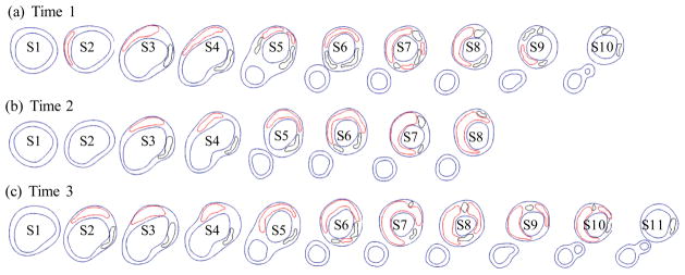
Serial MRI data from one patient was provided by the University of Washington (UW) group using protocols approved by the University of Washington Institutional Review Board with informed consent obtained. Scan time intervals were about 18 months, subject to scheduling variations. MRI scans were conducted on a GE SIGNA 1.5-T whole body scanner using an established protocol outlined in the papers by Yuan and Kerwin et al. [Kerwin, Hooker, Spilker, Vicini, Ferguson, Hatsukami, and Yuan (2003); Yuan and Kerwin (2004)]. Upon completion of a review, an extensive report was generated and segmented contour lines for different plaque components for each slice were sent to Tang’s group for model construction and further computational mechanical analysis. Details of the model construction process can be found from [Yang et al. (2007); Tang et al. (2008)]. Figure 1 gives the re-constructed 3D geometries of the plaque at three time points showing plaque progression. Figure 2 gives segmented contour plots of the plaque at three time points. 5 selected slices. These slices were used for model construction. The matched 8 slices were used to determine plaque growth functions. Plaque geometry at Time 3 was also used to validate simulated plaque progression.

Figure 1.

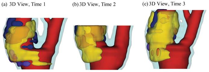
Re-constructed 3D geometry of a carotid plaque based on in vivo serial MRI data. Three time point data are shown. T1, T2 and T3 refer to time points from here on, unless otherwise indicated. Scan interval: T1–T2, 642 days; T2–T3, 519 days. Red – lumen; Cyan-outer wall; Yellow - necrotic core; Fresh red - hemorrhage in necrotic core); Purple - loose matrix; Dark blue – calcification; Green - fibrous cap.

Figure 2.

Segmented contour plots of a carotid plaque at three time points from a participating patient obtained from multi-weighting MRI slices. Carotid bifurcation was used as the registration point to match slices and 8 matched slices (S1–S8) were selected for this progression simulation study. Red: necrotic lipid core; Black: calcification.

2.2 The 3D Structure Model and Boundary Conditions

Since there was insufficient data to quantify individual plaque component growth, the plaque was treated as a uniform material, which was assumed to be linear, isotropic, incompressible and homogeneous. The governing equations and corresponding initial and boundary conditions are given below [Fung (1993;1994)]:

$$\rho u_{i,tt}={\sigma }_{ij,j},i,j=1,2,3;\text{sum}\text{over}j,$$ (1)

$${\epsilon }_{ij}=(u_{i,j}+u_{j,i})/2,i,j=1,2,3,$$ (2)

$${\sigma }_{ij}·n_j{\mid }_{\mathit{out}\_\mathit{wall}}=0,$$ (3)

$${\sigma }_{ij}·n_j{\mid }_{\mathrm{\Gamma }}=P_{in}(t){\mid }_{\mathrm{\Gamma }},$$ (4)

$$u_{i\mid t=0}=u_{i0},$$ (5)

$$u_{i,t\mid t=0}={\stackrel{.}{u}}_{i0},$$ (6)

$$u_3{\mid }_{z=0}=u_{30},$$ (7)

$$u_3{\mid }_{z=L}=u_{3L},$$ (8)

where ρ is vessel material density, (u₁, u₂, u₃) is the displacement vector corresponding to x,, and z directions, with z being the axial (longitudinal) direction. σ is stress tensor, ε is strain tensor, P_in is the specified lumen pressure, Γ is vessel inner boundary, u₃₀(t), u_3L(t) are the pre-stretch functions for the z-displacement at the two ends of the tube, f, j stands for derivative of f with respect to the jth variable. For the 3D linear model, the strain-stress relationship is:

$$\left(\begin{array}{l}{\sigma }_{11}\hfill \\ {\sigma }_{22}\hfill \\ {\sigma }_{33}\hfill \\ {\sigma }_{12}\hfill \\ {\sigma }_{23}\hfill \\ {\sigma }_{31}\hfill \end{array}\right)=D·\left(\begin{array}{l}{\sigma }_{11}\hfill \\ {\sigma }_{22}\hfill \\ {\sigma }_{33}\hfill \\ {\sigma }_{12}\hfill \\ {\sigma }_{23}\hfill \\ {\sigma }_{31}\hfill \end{array}\right)$$ (9)

$$D=\left(\begin{array}{cccccc}\lambda +2G& \lambda & \lambda & 0& 0& 0\\ \lambda & \lambda +2G& \lambda & 0& 0& 0\\ \lambda & \lambda & \lambda +2G& 0& 0& 0\\ 0& 0& 0& G& 0& 0\\ 0& 0& 0& 0& G& 0\\ 0& 0& 0& 0& 0& G\end{array}\right)$$ (10)

where

$$G=\frac{E}{2(1+\mu )},\lambda =\frac{E\mu }{(1+\mu )(1-2\mu )},$$ (11)

E is the Young’s Modulus, μ is the Poisson ratio which was set to 0.495 in this paper. Substitute (9)–(10) into (1), we have the displacement equations:

$$\rho \frac{{\partial }^2{u}_1}{\partial t^2}=(\lambda +2G)\frac{{\partial }^2{u}_1}{\partial x_1^2}+G(\frac{{\partial }^2{u}_1}{\partial x_2^2}+\frac{{\partial }^2{u}_1}{\partial x_3^2})+(\lambda +G)(\frac{{\partial }^2{u}_2}{\partial x_1{x}_2}+\frac{{\partial }^2{u}_3}{\partial x_1{x}_3})$$ (12)

$$\rho \frac{{\partial }^2{u}_2}{\partial t^2}=(\lambda +2G)\frac{{\partial }^2{u}_2}{\partial x_2^2}+G(\frac{{\partial }^2{u}_2}{\partial x_1^2}+\frac{{\partial }^2{u}_2}{\partial x_3^2})+(\lambda +G)(\frac{{\partial }^2{u}_1}{\partial x_1{x}_2}+\frac{{\partial }^2{u}_3}{\partial x_2{x}_3}),$$ (13)

$$\rho \frac{{\partial }^2{u}_3}{\partial t^2}=(\lambda +2G)\frac{{\partial }^2{u}_3}{\partial x_3^2}+G(\frac{{\partial }^2{u}_3}{\partial x_1^2}+\frac{{\partial }^2{u}_3}{\partial x_2^2})+(\lambda +G)(\frac{{\partial }^2{u}_1}{\partial x_1{x}_3}+\frac{{\partial }^2{u}_2}{\partial x_2{x}_3}).$$ (14)

The boundary conditions are:

$$[(\lambda +2G)\frac{\partial u_1}{\partial x_1}+\lambda (\frac{\partial u_2}{\partial x_2}+\frac{\partial u_3}{\partial x_3})]·n_1+G(\frac{\partial u_1}{\partial x_2}+\frac{\partial u_2}{\partial x_1})·n_2+G(\frac{\partial u_1}{\partial x_3}+\frac{\partial u_3}{\partial x_1})·n_3={\overline{t}}_1,$$ (15)

$$G(\frac{\partial u_1}{\partial x_2}+\frac{\partial u_2}{\partial x_1})·n_1+[(\lambda +2G)\frac{\partial u_2}{\partial x_2}+\lambda (\frac{\partial u_1}{\partial x_1}+\frac{\partial u_3}{\partial x_3})]·n_2+G(\frac{\partial u_2}{\partial x_3}+\frac{\partial u_3}{\partial x_2})·n_3={\overline{t}}_2,$$ (16)

$$G(\frac{\partial u_1}{\partial x_3}+\frac{\partial u_3}{\partial x_1})·n_1+G(\frac{\partial u_2}{\partial x_3}+\frac{\partial u_3}{\partial x_2})·n_2+[(\lambda +2G)\frac{\partial u_3}{\partial x_3}+\lambda (\frac{\partial u_1}{\partial x_1}+\frac{\partial u_2}{\partial x_2})]·n_3={\overline{t}}_3,$$ (17)

where (n₁, n₂, n₃) is the normal direction of the vessel surface. In our model, the inner boundary (lumen surface) is with (t̄₁, t̄₂, t̄₃) = (P_inn₁, P_inn₂, P_inn₃), P_in is the specified inner pressure. The outer boundary was set as a free boundary, with (t̄₁, t̄₂, t̄₃) = 0.

2.3 The Meshless Generalized Finite Difference Method (GFDM)

Meshless generalized finite difference (GFD) methods have been used in many engineering applications where irregular geometries and free-moving boundaries are involved [Kleiber (1998); Liszka and Orkisz (1980)]. The advantage of GFD method is that generalized finite difference schemes can be derived using arbitrarily distributed points (see Fig. 4). With GFD, we will be able to use denser nodal point distributions where plaque has higher stress/strain concentration or critical morphological features. We will also be able to adjust, move, add or drop nodal points as needed. This leads to the desired flexibility in handling the complex geometry and plaque growth where not only the geometry changes, the total plaque area (volume if 3D) also changes.

Figure 4.

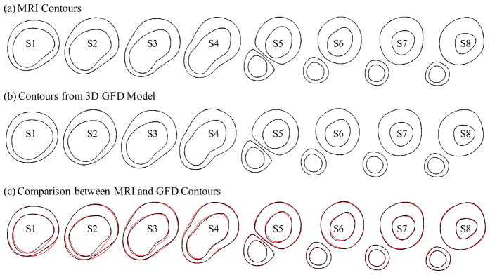
Comparison of MRI contours and GFD results after the shrink-stretch process. (a) MRI contour plots; (b) Contours from GFD model; (c) Comparison between MRI and GFD contours. Black: MRI; Red: GFD.

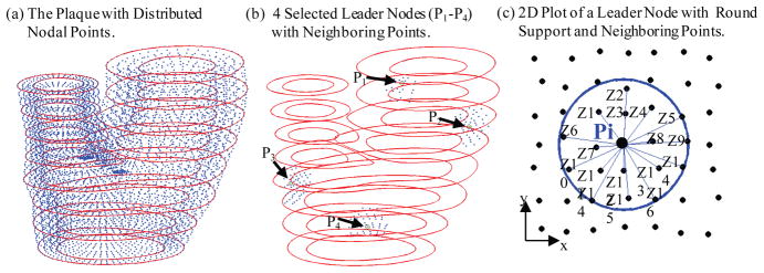
The GFD concept and derivation of the generalized finite difference schemes are explained by the following example. Fig. 3(a) gives the carotid plaque with distributed nodal points. Fig. 3(b) gives 4 leader-nodes (Pi) with their neighbor nodes (Zj). One leader node was a boundary node. The other 3 were inner nodes. The neighbor nodes were selected using a sphere support with radius: R = s*max (dx, dy, dz). The support size control data s = 3.0 was determined numerically to reach best agreement with solutions obtained by ADINA. Fig. 3(c) shows a simplified 2D plot of a leader node with its neighboring points, illustrating the derivation process of GFD scheme.

Figure 3.

Schematic drawing of meshless GFD scheme derivation and nodal point distributions. (a) The plaque with distributed nodal points; (b) 4 selected leader nodes with round support and neighboring points; (c) 2D plot of a leader node with round support and neighboring points (Zj) for easy viewing.

For inner nodes, we use 2^nd order GFD scheme. For boundary nodes, we use 1^st order GFD scheme. For each leader node Pi with Ni neighbor nodes Z_j, j = 1, …, N_i (see Fig. 3(c)), the 2^nd order Taylor expansion of f (x, y, z) at P_i is given by:

$$f_j=f_{Pi}+{dx}_j{\frac{\partial f}{\partial x_1}|}_{Pi}+{dy}_j{\frac{\partial f}{\partial x_2}|}_{Pi}+{dz}_j{\frac{\partial f}{\partial x_3}|}_{Pi}+{\frac{{dx}_j^2}{2}\frac{{\partial }^{2}f}{\partial x_1^2}|}_{Pi}+{\frac{{dy}_j^2}{2}\frac{{\partial }^{2}f}{\partial x_2^2}|}_{Pi}+{\frac{\partial z_j^2}{2}\frac{{\partial }^{2}f}{\partial x_3^2}|}_{Pi}+{dx}_j{dy}_j{\frac{{\partial }^{2}f}{\partial x_1{x}_2}|}_{Pi}+{dy}_j{dz}_j{\frac{{\partial }^{2}f}{\partial x_2{x}_3}|}_{Pi}+{dx}_j{dz}_j{\frac{{\partial }^{2}f}{\partial x_1{x}_3}|}_{Pi}+o({dx}_j^2+{dy}_j^2+{dz}_j^2),$$ (18)

where the subscript j = 1… Ni is the subscript for the neighbor nodes Zj of Pi. f is u₁, u₂, u₃ in displacement formula, f_j = f (Zj). Dropping the last term, we have:

$$\left(\begin{array}{ccccccccc}d{x}_1& d{y}_1& d{z}_1& \frac{d{x}_1^2}{2}& \frac{d{y}_1^2}{2}& \frac{d{z}_1^2}{2}& d{x}_{1}d{y}_1& d{y}_{1}d{z}_1& d{x}_{1}d{z}_1\\ ⋮& ⋮& ⋮& ⋮& ⋮& ⋮& ⋮& ⋮& ⋮\\ d{x}_{Ni}& d{y}_{Ni}& d{z}_{Ni}& \frac{d{x}_{Ni}^2}{2}& \frac{d{y}_{Ni}^2}{2}& \frac{d{z}_{Ni}^2}{2}& d{x}_{Ni}d{y}_{Ni}& d{y}_{Ni}d{z}_{Ni}& d{x}_{Ni}d{z}_{Ni}\end{array}\right)·{\left(\begin{array}{c}{f}_{,1}\\ f_{,2}\\ f_{,3}\\ f_{,11}\\ f_{,22}\\ f_{,33}\\ f_{,12}\\ f_{,23}\\ f_{,13}\end{array}\right)}_{Pi}=\left(\begin{array}{c}{f}_1-f_{Pi}\\ ⋮\\ f_{Ni}-f_{Pi}\end{array}\right)$$ (19)

where f_j = f (Zj), $f_{,k}=\frac{\partial f}{\partial x_k}·f_{,kl}=\frac{{\partial }^{2}f}{\partial x_k\partial x_l}$. GFD schemes for all the first and second order derivatives are determined from (19) using function values at the Ni neighbor nodes and least-square approximation techniques.

The first-order Taylor expansion is given by:

$$f_j=f_{Pi}+d{x}_j{\frac{\partial f}{\partial x_1}|}_{Pi}+d{y}_j{\frac{\partial f}{\partial x_2}|}_{Pi}+d{z}_j{\frac{\partial f}{\partial x_3}|}_{Pi}+o(d{x}_j+d{y}_j+d{z}_j).$$ (20)

The first order GFD schemes can be obtained similarly from the following system:

$$\left(\begin{array}{ccc}d{x}_1& d{y}_1& d{z}_1\\ ⋮& ⋮& ⋮\\ d{x}_{Ni}& d{x}_{Ni}& d{x}_{Ni}\end{array}\right)·{\left(\begin{array}{c}{f}_{,1}\\ f_{,2}\\ f_{,3}\end{array}\right)}_{Pi}=\left(\begin{array}{c}{f}_1-f_{Pi}\\ ⋮\\ f_{Ni}-f_{Pi}\end{array}\right)$$ (21)

2^nd order center difference scheme was used for the time derivative term:

$$\frac{{\partial }^{2}f}{\partial t^2}=\frac{f^{n+1}-2f^n+f^{n-1}}{\mathrm{\Delta }{t}^2}+o(\mathrm{\Delta }{t}^2)$$ (22)

Substituting all the GFD schemes and (22) into (12)–(14), we obtained the final linear system for the displacement function:

$$K\overrightarrow{u}=\overrightarrow{f}.$$ (23)

The vector = (u₁, u₂, u₃)^T is the displacement solution at time step (n + 1).

2.4 3D Re-Construction, Shrink-Stretch Process, and GFD Method Validation

Under the in vivo condition, the artery is axially stretched and pressurized, thus axial and circumferential shrinking was needed a priori to generate the starting plaque geometry for the computational model. The shrinkage in axial direction was 9% so that the vessel would regain its in vivo length with a 10% axial stretch. Circumferential shrinkage for lumen and outer wall was determined so that: 1) total mass volume was conserved; 2) plaque geometry after 10% axial stretch and pressurization had the best match with the original in vivo geometry. Steady pressure condition Pin = 100 mm Hg was used in the model. The Young’s modulus was set to E = 3.6e + 6 = 360 KPa based on our experimental data [Kobayashi, Tsunoda, Fukuzawa, Morikawa, Tang, Ku (2003); Tang et al. (2008); Tang, Yang, Zheng, Woodard, Saffitz, Petruccelli, Sicard and Yuan (2005)] and current literature [Fung (1993); Humphrey (2002)]. Fig. 4 compares the contours obtained from the GFD model with MRI contours. While some variation can be observed due to the stretch and pressurization, the net wall thickness errors (averaged over all 1200 data points) were less than 2%.

A commercial finite element software package ADINA (ADINA R & D, Inc., Watertown, MA) was used to validate our GFD model. ADINA has been validated by hundreds of realistic engineering and real life applications and is well accepted in the industry and research communities [Bathe (1996); Bathe (2002)]. We have been using ADINA in the past 12 years to construct and solve 2D/3D artery models which were validated by experimental measurements [Tang et al. (2005, 2008)]. Finite element ADINA models were constructed for all three time points T1, T2 and T3 following the same procedures using in [Tang et al. (2005)]. Comparisons of results from the two models are given in Section 3.

2.5 Vessel Wall Thickness Definition and Quantification of Plaque Growth Functions

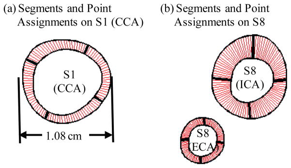
Plaque GFD models were constructed based on in vivo MRI data at Time 1 (T1), Time 2 (T2) and Time 3 (T3) and solved to get 3D plaque geometry (which matched in vivo MRI geometry with errors less than 2%) and stress/strain data. Slices from the three scans (T1, T2 and T3) were matched using the carotid bifurcation as the registration point (see Fig. 2). In this paper, vessel wall thickness (WT) was selected as the measure for plaque progression. For each matched slice, 100 evenly-spaced points from the lumen were selected and a piecewise equal-step method was introduced to calculate wall thickness (Fig. 5). Each slice was divided into several segments according to its geometry (4 for this plaque sample). For each segment, equal step is used for inner and outer boundaries respectively to choose equal number of nodal points. The corresponding points on the inner and out boundaries are paired and the distance between the paired points are defined as vessel wall thickness at the given lumen point (Fig. 5). This method is sufficient for the cases covered in this paper.

Figure 5.

Piecewise equal-step method for vessel wall thickness definition. (a) Segments and point assignments on Slice 1; (b) Segments and point assignments on Slice 8. CCA = common carotid artery. ECA = external carotid artery. ICA = internal carotid artery.

Using the plaque geometry and stress data at T1 and T2, four plaque growth functions (GF1, …, GF4) were introduced to predict “next time step” plaque geometry:

$$GF1(i,j)=a_0(j)+a_1(j)\times f_{T2}(i,j)+a_2(j)\times {\frac{df}{dt}|}_{T2}(i,j)·\mathrm{\Delta }t,$$ (24)

$$GF2(i,j)=a_0(j)+a_1(j)\times f_{T2}(i,j)+a_2(j)\times f_{T2}(i-1,j)+a_3(j)\times f_{T2}(i+1,j)+a_4(j)\ast {\frac{df}{dt}|}_{T2}(i,j)·\mathrm{\Delta }t,$$ (25)

$$GF3(i,j)=a_0(j)+a_1(j)\times f_{T2}(i,j)+a_2(j)\times {\frac{df}{dt}|}_{T2}(i,j)·\mathrm{\Delta }t+a_3(j)\times {\sigma }_{T2}(i,j)+a_4(j)\times {\frac{d\sigma }{dt}|}_{T2}(i,j)·\mathrm{\Delta }t,$$ (26)

$$GF4(i,j)=a_0(j)+a_1(j)\times f_{T2}(i,j)+a_2(j)\times f_{T2}(i-1,j)+a_3(j)\times f_{T2}(i+1,j)+a_4(j)\times {\frac{df}{dt}|}_{T2}(i,j)·\mathrm{\Delta }t+a_5(j)\times {\sigma }_{T2}(i,j)+a_6(j)\times {\frac{d\sigma }{dt}|}_{T2}(i,j)·\mathrm{\Delta }t,$$ (27)

where a_k(j) are coefficients of the growth functions to be determined using T3 data, f can be displacement variables or wall thickness, σ is the maximum principal stress at the nodal point, ${\frac{df}{dt}|}_{T2}(i,j)=\frac{f_{T2}(i,j)-f_{T1}(i,j)}{T2-T1}$ which could also be calculated using numerical steps in the simulation, Δt = time step in simulation, j = 1, 2, … 8 is the slice number, i is the index for the points on each slice. GF1 uses wall thickness at one nodal point x_i only. GF2 added neighboring points x_i−1 and x_{i + 1} to GF1. GF3 included both WT and stress. GF4 added neighboring points x_i−1 and x_{i + 1} to GF3.

Nodal positions of the selected 1200 nodal point pairs (100 per lumen including CCA, ECA and ICA) on plaque inner and outer boundaries obtained from the GFD model at T3 were used to determined the coefficients a_k(j) in GF1-GF4. Least square approximations were used to reach the best fit. R² values of the fitting results are given in Table 1.

Table 1.

R² values of the least-squares fitting results using the four growth functions. (x-in, y-in) are coordinates of inner (lumen) boundary points. (x-out, y-out) are coordinates of out boundary points.

GF	Feature	x-in	y-in	x-out	y-out
GF1	WT	0.997308	0.997525	0.996558	0.994908
GF2	WT + Neighbor	0.999483	0.999425	0.999225	0.999375
GF3	WT + Stress	0.998392	0.998283	0.997542	0.996850
GF4	WT + Stress + Neighbor	0.999742	0.999600	0.999533	0.999592

2.6 Plaque Progression Simulation

Starting from the plaque geometry at T2 and using the plaque growth functions determined in 2.5, the following procedure was used to simulate plaque progression and try to reach best agreement with plaque geometry at T3 obtained from GFD model (called the target T3 geometry from here on):

• Step 1. Start from the original in vivo MRI geometry at T2, use proper shrinkage to get the zero-pressure numerical starting geometry;

• Step 2. Discretize the geometry using the meshless GFD method, solve the model to get plaque geometry and stress/strain distributions under specified pressure conditions;

• Step 3. Set

  $$f_{T2\_0}(i,j)=f_{T2}(i,j),$$ (28)

  $$f_{T2\_1}(i,j)=f_{T2}(i,j)+(f_{T3}(i,j)-f_{T2}(i,j))/m,$$ (29)

• Step 4. We use m time steps to go from T2 to T3. For K = 1, …, m−1, do the following (use GF1 as an example, GF2–GF4 are similar)

• Step 4-1:

  $$f_{T2\_(k+1)}(i,j)=a_0(j)+a_1(j)\times [w\ast f_{T2\_k}(i,j)+(1-w)f_{T2}(i,j)]+a_2(j)\ast {\frac{df}{dt}|}_{T2\_k}(i,j)·\mathrm{\Delta }{t}_k],$$ (30)

  where ${\frac{df}{dt}|}_{T2\_k}(i,j)=\frac{f_{T2\_k}(i,j)-f_{T2\_\text{(}k-1)}(i,j)}{t_k-t_{k-1}},\mathrm{\Delta }{t}_k=t_{k+1}-t_k=\frac{T3-T2}{m}$, f is the x and y coordinates of nodal points of inner and outer boundaries for each slice.

• Step 4-2. Adjust internal nodal points as needed;

• Step 4-3. Solve the plaque model using the updated plaque geometry;

• Step 4-4. Repeat Steps 4-1 to 4-3 till numerical time reaches T3.

The neighboring points and stress terms in GF2–GF4 were handled in similar ways. The w-value in the simulation formula was determined numerically to have the best matching with plaque T3 geometry. Results obtained from the simulation code are presented in next section.

3 Results

One patient data with three time point MRI scans was used to construct the GFD models and demonstrate the simulation process. Results from GFD models were compared with that from ADINA models for model and method validation. Simulation errors from the four selected growth functions were compared. Details are given below.

3.1 3D Meshless GFD Methods Provided Good Agreement with ADINA Solutions

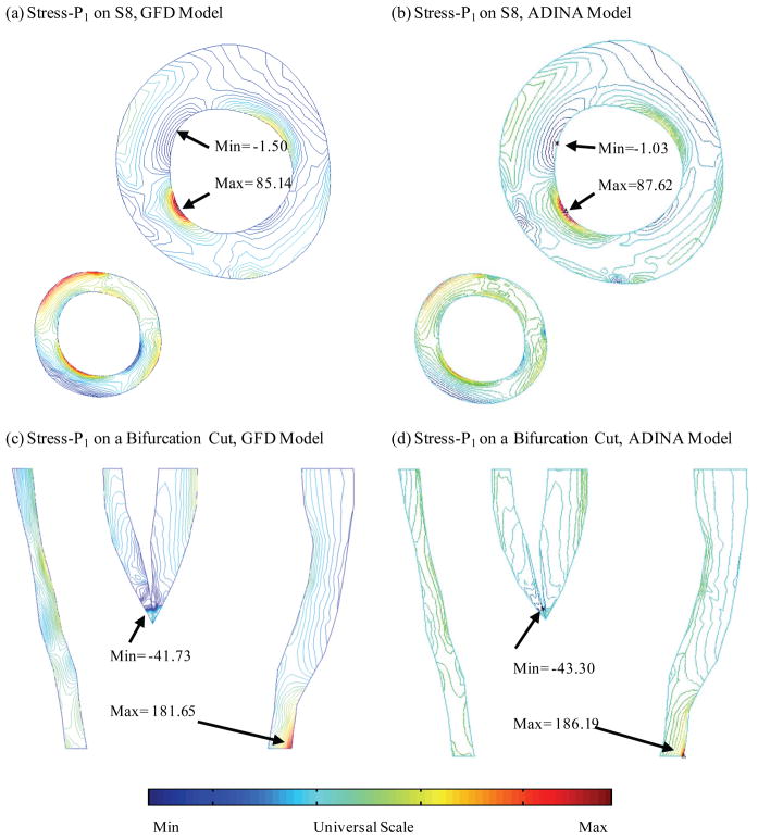
Figure 6 compares plaque maximum principal stress (Stress-P₁) obtained from both GFD and ADINA models on slice S8 and on a bifurcation cut surface. GFD results agreed well with ADINA results (error < 3%).

Figure 6.

GFD model validation: Comparison of plaque maximum principal stress (Stress-P1) from GFD and ADINA models on Slice 8 and a bifurcation cut surface indicates that GFD Stress-P1 solution has a good agreement with that from ADINA model (error < 3%).

3.2 Plaque Progression Simulation Using Growth Function GF1

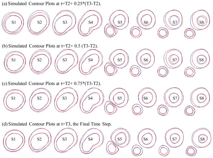
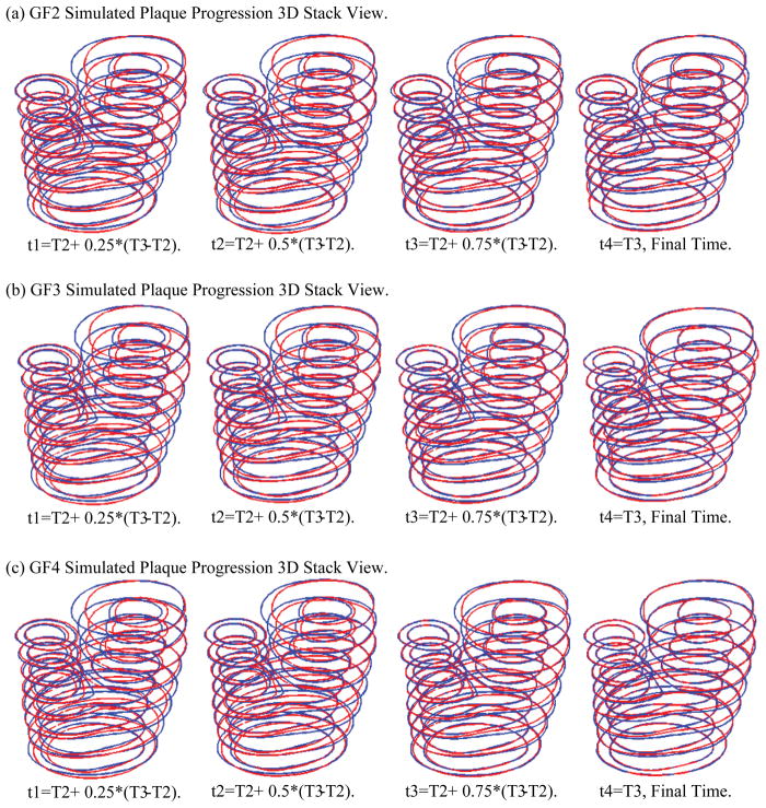
Four growth functions were used to simulate plaque progression from T2 to T3 following the procedure described in 3.3. Fig. 7 gives the overlapping contour plots of the simulated results at t = T2 + (T3 − T2)/4, T2 + (T3 − T2)/2, T2 + 3*(T3 − T2)/4, and T3, showing good agreement between simulated and actual plaque progression. Fig. 8 gives the 3D stacked view of the simulated plaque geometries at 4 time steps.

Figure 7.

Simulated contour plots at 4 intermediate time steps compared with the target T3 plaque contours as T3. Blue: target contours (plaque geometry at T3 obtained from GFD model); Red: simulated plaque contours converging to the target contours).

Figure 8.

3D view of simulated plaque geometries converging to the target geometry.

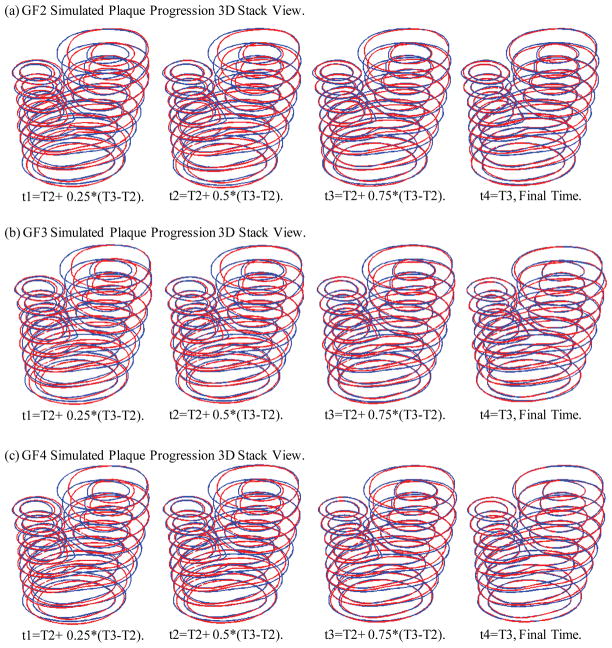
Fig. 9 shows 3D stack views of simulated plaque progression using GF2, GF3, and GF4. It is clear that GF2 and GF4 (with neighboring points) provided better agreement with the target T3 geometry, compared to GF1 and GF3, respectively. Similarly, GF3 and GF4 using both wall thickness and stress data led to better match with target T3 geometry than that given by GF1 and GF2.

Figure 9.

3D stack view of simulated plaque progression geometries using three growth functions GF2, GF3, and GF4 showing including neighboring points and stress terms led to better match with target T3 geometry.

To quantitatively compare the errors associated the four growth functions, we define the absolute and relative errors as:

$$\text{Absolute}\text{Error}=\mathrm{\sum }\mid \text{Simulated}WT(i)-\text{Target}WT\_T3(i)\mid /1200,$$ (31)

$$\text{Relative}\text{Error}=\text{Absolute}\text{Error}/\text{Average}\text{Wall}\text{Thick}\text{at}T3,$$ (32)

$$\text{Average}\text{Wall}\text{Thickness}=\mathrm{\sum }WT\_T3(i)/1200,$$ (33)

where 1200 = total number of nodal points selected from inner boundary, target WT_T3 is the plaque wall thickness at T3 obtained from GFD model with axial stretch and pressure applied to reach best match with MRI geometry. The errors for the simulated plaque geometries using GF1–GF4 are given by Table 2. GF4 gave the best match with the target T3 geometry, which is 4.45%, only about 1/3 of the error given by GF1.

Table 2.

Growth function with neighboring points and stress terms provided much better agreement with the target T3 geometry.

Growth Function	GF1	GF2	GF3	GF4
Average T3 WT (cm)	0.15857	0.15857	0.15857	0.15857
Absolute Error (cm)	0.01833	0.01014	0.01307	0.00706
Relative Error	11.56%	6.39%	8.24%	4.45%

4 Discussion

4.1 Mechanisms Governing Plaque Progression and Computational Simulation

It is well-known that atherosclerotic plaque progression is a multi-faceted process involving not only mechanical factors, but also plaque type, component size and location, inflammation and lumen surface condition, biological processes including many different cell activities, blood conditions such as cholesterol level, diabetes, changes caused by medication, diet, life styles, exercise, emotions, etc. To reproduce the realistic plaque progression process accurately, we need to know the real mechanisms governing the progression and real-time information about all the factors involved in the process. To be honest, little is known about real human plaque progression mechanisms based on patient-tracking data. And it is absolutely impossible to have complete real-time patient-tracking data for the duration of plaque progression to its maturity (up to 50 years). Investigations and findings from all the channels, modalities and disciplines could be integrated together to obtain better and more thorough understanding of the complicated atherosclerotic progression process. Our computational simulation approach takes the actual multi-year plaque progression data to simulate future growth, based on the assumptions that the trend that led to the current state would continue into the future. In other words, the governing mechanisms (whether we know them or not) would remain the same: the contributing factors would continue to contribute the same way as they did in the past, with the changes taken into consideration by the terms included in the plaque growth function.

Our results indicated that the growth function with neighboring points and structural stress included provided better matching with the target geometry, with an error of 4.45%, compared to an error of 11.56% given by a growth function without neighboring points and structural stress terms. It is reasonable to expect that growth functions including flow shear stress, blood chemical conditions, cholesterol level and other related factors may lead to better progression simulation results.

4.2 Significance of the Meshless GFD Method

Human atherosclerotic plaques have complex geometries. Mesh generation will take considerable effort to build a finite element plaque model. Plaque progression simulation requires that plaque geometry be adjusted for each numerical time step. One major limitation of finite element models or other similar models which involve mesh generation is that re-meshing of the structure domain is extremely time consuming and hard to be automated. This makes mesh-based simulation code for progression simulation near impossible. By using the meshless GFD method, we can adjust computational nodes in the plaque anyway we want to grow the plaque as the growth function dictates. And this can be written into the computational code so that it is done automatically. The method and model developed in this paper can be applied to many other biological and engineering processes where the computational domain changes in the process being investigated.

4.3 Model limitations

Clearly the current model is very limited and serves as initial demonstrations of the GFD method and the potential significant contributions from the progression simulation model. The material model needs to be extended to 3D nonlinear models to reflect artery stiffening behaviors. Plaque components should be included in the model. Fluid-structure interactions should be added. And the growth functions need to be adjusted to include fluid shear stress, blood chemical conditions, and the proper terms that can represent the plaque growth trend. Better understanding of the biological and mechanical factors will help us to better formulate the growth function.

5 Conclusion

We believe that this is the first time that 3D human carotid atherosclerotic plaque progression was simulated based on patient-specific plaque morphology and pointwise plaque growth functions derived from multi-year MRI data. Our results indicated that our proposed progression simulation process was able to accurately predict future plaque morphology if the current progression trend was continued. The 3D meshless GFD method worked well for the progression model. The predicted progression by the growth function including neighboring points and structural stress terms was considerably more accurate than that given by other growth functions. The current 3D structure model can be extended to 3D model with fluid-structure interactions and more terms can be added to the growth functions for better predictions. More case studies are needed to validate our findings. Accurate plaque progression simulation adds the time dimension to plaque vulnerability assessment strategies and should improve our predicting accuracies.

References

- Ahrem R, Beckert A, Wendland H. A meshless spatial coupling scheme for large-scale fluid-structure-interaction problems. CMES: Computer Modeling in Engineering & Sciences. 2006;12(2):121–136. [Google Scholar]
- Atluri SN. Methods of Computer Modeling in Engineering & the Sciences-Part I. Tech Science Press; Forsyth, GA: 2005. [Google Scholar]
- Atluri SN. The Meshless Local-Petrov-Galerkin Method for Domain & BIE Discretizations. Tech Science Press; Forsyth, GA: 2004. [Google Scholar]
- Atluri SN, Han ZD, Rajendran AM. A new implementation of the meshless finite volume method, through the MLPG “Mixed” approach. CMES: Computer Modeling in Engineering & Sciences. 2004;6(6):491–513. [Google Scholar]
- Atluri SN, Liu HT, Han ZD. Meshless local Petrov-Galerkin (MLPG) mixed collocation method for elasticity problems. CMES: Computer Modeling in Engineering & Sciences. 2006a;14(3):141–152. [Google Scholar]
- Atluri SN, Liu HT, Han ZD. Meshless local Petrov-Galerkin (MLPG) mixed finite difference method for solid mechanics. CMES: Computer Modeling in Engineering & Sciences. 2006b;15(1):1–16. [Google Scholar]
- Atluri SN, Yagawa G, Cruse TA, editors. Computational Mechanics ’95. I & II. Springer-Verlag; New York: 1995. [Google Scholar]
- Bathe KJ. Finite Element Procedures. Prentice Hall, Inc; New Jersey: 1996. [Google Scholar]
- Bathe KJ, editor. Theory and Modeling Guide. I & II. ADINA and ADINA-F, ADINA R & D, Inc; Watertown, MA: 2002. [Google Scholar]
- Cai YC, Zhu HH. A local meshless Shepard and least square interpolation method based on local weak form. CMES: Computer Modeling in Engineering & Sciences. 2008;34(2):179–204. [Google Scholar]
- Colli S, Gei M, Bigoni D. A boundary element formulation for incremental nonlinear elastic deformation of compressible solids. CMES: Computer Modeling in Engineering & Sciences. 2009;40(1):29–62. [Google Scholar]
- Friedman MH, Bargeron CB, Deters OJ, Hutchins GM, Mark FF. Correlation between wall shear and intimal thickness at a coronary artery branch. Atherosclerosis. 1987;68:27–33. doi: 10.1016/0021-9150(87)90090-6. [DOI] [PubMed] [Google Scholar]
- Friedman MH, Giddens DP. Blood flow in major blood vessels - modeling and experiments. Annals of Biomedical Engineering. 2005;33(12):1710–1713. doi: 10.1007/s10439-005-8773-1. [DOI] [PubMed] [Google Scholar]
- Fung YC. A First Course in Continuum Mechanics. 3. Englewood Cliffs; New Jersey: 1994. [Google Scholar]
- Fung YC. Biomechanics: Mechanical properties of Living Tissues. Springer-Verlag; New York: 1993. p. 68. [Google Scholar]
- Fuster V. The Vulnerable Atherosclerotic Plaque: Understanding, Identification, and Modification. In: Fuster V, Cornhill JF, Dinsmore RE, Fallon JT, Insull W, Libby P, Nissen S, Rosenfeld ME, Wagner WD, editors. AHA Monograph series. Futura Publishing; Armonk NY: 1998. [Google Scholar]
- Fuster V, Stein B, Ambrose JA, Badimon L, Badimon JJ, Chesebro JH. Atherosclerotic plaque rupture and thrombosis, evolving concept. Circulation. 1990;82(Supplement II):II-47–II-59. [PubMed] [Google Scholar]
- Gibson CM, Diaz L, Kandarpa K, Sacks FM, Pasternak RC, Sandor T, Feldman C, Stone PH. Relation of vessel wall shear stress to atherosclerosis progression in human coronary arteries. Arterioscler Thromb. 1993;13(2):310–5. doi: 10.1161/01.atv.13.2.310. [DOI] [PubMed] [Google Scholar]
- Giddens DP, Zarins CK, Glagov S. The role of fluid mechanics in the localization and detection of atherosclerosis. Journal of Biomechanical Engineering. 1993;115:588–594. doi: 10.1115/1.2895545. [DOI] [PubMed] [Google Scholar]
- Han ZD, Atluri SN. Meshless local Petrov-Galerkin (MLPG) approaches for solving 3D problems in elasto-statics. CMES: Computer Modeling in Engineering & Sciences. 2004a;6(2):169–188. [Google Scholar]
- Han ZD, Atluri SN. A meshless local Petrov-Galerkin (MLPG) approach for 3-dimensional elasto-dynamics. CMC: Computers, Materials & Continua. 2004b;1(2):129–140. [Google Scholar]
- Han ZD, Atluri SN. A Systematic Approach for the Development of Weakly–Singular BIEs. CMES: Computer Modeling in Engineering & Sciences. 2007;21(1):41–52. [Google Scholar]
- Han ZD, Liu HT, Rajendran AH, Atluri SN. The Applications of Meshless Local Petrov-Galerkin (MLPG) Approaches in High-Speed Impact, Penetration and Perforation Problems. CMES: Computer Modeling in Engineering & Sciences. 2006;14(2):119–128. [Google Scholar]
- Han ZD, Rajendran AM, Atluri SN. Meshless local Petrov-Galerkin (MLPG) approaches for solving nonlinear problems with large deformations and rotations. CMES: Computer Modeling in Engineering & Sciences. 2005;10(1):1–12. [Google Scholar]
- Hu SP, Young DL, Fan CM. FDMFS for Diffusion Equation with Unsteady Forcing Function. CMES: Computer Modeling in Engineering & Sciences. 2008;24(1):1–20. [Google Scholar]
- Humphrey JD. Cardiovascular Solid Mechanics. Springer-Verlag; New York: 2002. [Google Scholar]
- Kerwin W, Hooker A, Spilker M, Vicini P, Ferguson M, Hatsukami T, Yuan C. Quantitative magnetic resonance imaging analysis of neovasculature volume in carotid atherosclerotic plaque. Circulation. 2003;107(6):851–856. doi: 10.1161/01.cir.0000048145.52309.31. [DOI] [PubMed] [Google Scholar]
- Kleiber M. Handbook of Computational Solid Mechanics. Springer-Verlag; New York: 1998. [Google Scholar]
- Kobayashi S, Tsunoda D, Fukuzawa Y, Morikawa H, Tang D, Ku DN. Flow and compression in arterial models of stenosis with lipid core. Proceedings of 2003 ASME Summer Bioengineering Conference; Miami, FL. 2003. pp. 497–498. [Google Scholar]
- Ku DN, Giddens DP, Zarins CK, Glagov S. Pulsatile flow and atherosclerosis in the human carotid bifurcation: positive correlation between plaque location and low and oscillating shear stress. Arteriosclerosis. 1985;5:293–302. doi: 10.1161/01.atv.5.3.293. [DOI] [PubMed] [Google Scholar]
- Li S, Atluri SN. The MLPG mixed collocation method for material orientation and topology optimization of anisotropic solids and structures. CMES: Computer Modeling in Engineering & Sciences. 2008;30(1):37–56. [Google Scholar]
- Ling XW, Atluri SN. Stability analysis for inverse heat conduction problems. CMES: Computer Modeling in Engineering & Sciences. 2006;13(3):219–228. [Google Scholar]
- Liszka T, Orkisz J. The finite difference method at arbitrary irregular grids and its application in applied mechanics. Computers and Structures. 1980;11:83–95. [Google Scholar]
- Liu YH, Chen SS, Li J, Cen ZZ. A meshless local natural neighbor interpolation method applied to structural dynamic analysis. CMES: Computer Modeling in Engineering & Sciences. 2008;31(3):145–156. [Google Scholar]
- Lucas P, van Zuijlen AH, Bijl H. An automated approach for solution based mesh adaptation to enhance numerical accuracy for a given number of grid cells applied to steady flow on hexahedral grids. CMES: Computer Modeling in Engineering & Sciences. 2009;41(2):147–176. [Google Scholar]
- Ma QW. A New Meshless Interpolation Scheme for MLPG_R Method. CMES: Computer Modeling in Engineering & Sciences. 2008;23(2):75–90. [Google Scholar]
- Mai-Duy N, Tran-Cong T. Boundary integral-based domain decomposition technique for solution of Navier-Stokes equations. CMES: Computer Modeling in Engineering & Sciences. 2004;6(1):59–76. [Google Scholar]
- Masuda S, Noguchi H. Analysis of Structure with Material Interface by Meshfree Method. CMES: Computer Modeling in Engineering & Sciences. 2006;11(3):131–144. [Google Scholar]
- Naghavi M, Libby P, Falk E, Casscells SW, Litovsky S, Rumberger J, Badimon JJ, Stefanadis C, Moreno P, Pasterkamp G, Fayad Z, Stone PH, Waxman S, Raggi P, Madjid M, Zarrabi A, Burke A, Yuan C, Fitzgerald PJ, Siscovick DS, de Korte CL, Aikawa M, Juhani KE, Airaksinen KE, Assmann G, Becker CR, Chesebro JH, Farb A, Galis ZS, Jackson C, Jang IK, Koenig W, Lodder RA, March K, Demirovic J, Navab M, Priori SG, Rekhter MD, Bahr R, Grundy SM, Mehran R, Colombo A, Boerwinkle E, Ballantyne C, Insull W, Jr, Schwartz RS, Vogel R, Serruys PW, Hansson GK, Faxon DP, Kaul S, Drexler H, Greenland P, Muller JE, Virmani R, Ridker PM, Zipes DP, Shah PK, Willerson JT. From vulnerable plaque to vulnerable patient: a call for new definitions and risk assessment strategies: Part I. Circulation. 2003a;108(14):1664–72. doi: 10.1161/01.CIR.0000087480.94275.97. [DOI] [PubMed] [Google Scholar]
- Naghavi M. From vulnerable plaque to vulnerable patient: a call for new definitions and risk assessment strategies: Part II. Circulation. 2003b;108(15):1772–8. doi: 10.1161/01.CIR.0000087481.55887.C9. (co-authors are the same as above) [DOI] [PubMed] [Google Scholar]
- Perko J, Sarler B. Weight Function Shape Parameter Optimization in Meshless Methods for Non-uniform Grids. CMES: Computer Modeling in Engineering & Sciences. 2007;19(1):55–68. [Google Scholar]
- Scotti CM, Shkolnik AD, Muluk SC, Finol EA. Fluid-structure interaction in abdominal aortic aneurysms: effects of asymmetry and wall thickness. Biomed Eng Online. 2005;4:64–70. doi: 10.1186/1475-925X-4-64. [DOI] [PMC free article] [PubMed] [Google Scholar]
- Sellountos EJ, Sequeira A, Polyzos D. Elastic transient analysis with MLPG(LBIE) method and local RBFs. CMES: Computer Modeling in Engineering & Sciences. 2009;41(3):215–242. [Google Scholar]
- Shu C, Ding H, Yeo KS. Computation of incompressible Navier-Stokes equations by local RBF-based differential quadrature method. CMES: Computer Modeling in Engineering & Sciences. 2005;7(2):195–206. [Google Scholar]
- Sladek J, Sladek V, Solek P, Atluri SN. Modeling of intelligent material systems by the MLPG. CMES: Computer Modeling in Engineering & Sciences. 2008;34(3):273–300. [Google Scholar]
- Sladek J, Sladek V, Tan CL, Atluri SN. Analysis of transient heat conduction in 3D anisotropic functionally graded solids, by the MLPG Method. CMES: Computer Modeling in Engineering & Sciences. 2008;32(3):161–174. [Google Scholar]
- Song R, Chen W. An investigation on the regularized meshless method for irregular domain problems. CMES: Computer Modeling in Engineering & Sciences. 2009;42(1):59–70. [Google Scholar]
- Tang D, Chen XK, Yang C, Kobayashi K, Ku DN. A viscoelastic model and meshless GFD method for Blood Flow in collapsible Stenotic Arteries, Advances in Computational Engineering & Sciences. International Conference on Computational Engineering and Sciences.Tech Science Press; 2002. [Google Scholar]
- Tang D, Yang C, Kobayashi K, Ku DN. A Generalized Finite Difference Method for 3-D Viscous Flow in Stenotic Tubes with Large Wall Deformation and Collapse. Applied Num Math. 2001;38:49–68. [Google Scholar]
- Tang D, Yang C, Mondal S, Liu F, Canton G, Hatsukami TS, Yuan C. A Negative Correlation between Human Carotid Atherosclerotic Plaque Progression and Plaque Wall Stress: In Vivo MRI-Based 2D/3D FSI Models. J Biomechanics. 2008;41(4):727–736. doi: 10.1016/j.jbiomech.2007.11.026. [DOI] [PMC free article] [PubMed] [Google Scholar]
- Tang D, Yang C, Zheng J, Woodard PK, Saffitz JE, Petruccelli JD, Sicard GA, Yuan C. Local maximal stress hypothesis and computational plaque vulnerability index for atherosclerotic plaque assessment. Annals of Biomedical Engineering. 2005;33(12):1789–1801. doi: 10.1007/s10439-005-8267-1. [DOI] [PMC free article] [PubMed] [Google Scholar]
- Wacher A, Givoli D. Remeshing and Refining with Moving Finite Elements. Application to Nonlinear Wave Problems. CMES: Computer Modeling in Engineering & Sciences. 2006;15(3):147–164. [Google Scholar]
- Wu XH, Shen SP, Tao WQ. Meshless Local Petrov-Galerkin Collocation Method for Two-dimensional Heat Conduction Problems. CMES: Computer Modeling in Engineering & Sciences. 2007;22(1):65–76. [Google Scholar]
- Yang C, Tang D, Yuan C, Hatsukami TS, Zheng J, Woodard PK. In Vivo/Ex Vivo MRI-Based 3D Models with Fluid-Structure Interactions for Human Atherosclerotic Plaques Compared with Fluid/Wall-Only Models. CMES: Computer Modeling in Engineering & Sciences. 2007;19(3):233–245. [PMC free article] [PubMed] [Google Scholar]
- Yang C, Tang D, Yuan C, Kerwin W, Liu F, Canton G, Hatsukami TS, Atluri S. Meshless Generalized Finite Difference Method and Human Carotid Atherosclerotic Plaque Progression Simulation Using Multi-Year MRI Patient-Tracking Data. CMES: Computer Modeling in Engineering & Sciences. 2008;28(2):95–107. [PMC free article] [PubMed] [Google Scholar]
- Young DL, Chen KH, Liu TY, Shen LH, Wu CS. Hypersingular meshless method for solving 3D potential problems with arbitrary domain. CMES: Computer Modeling in Engineering & Sciences. 2009;40(3):225–270. [Google Scholar]
- Yuan C, Kerwin WS. MRI of atherosclerosis. Journal of Magnetic Resonance Imaging. 2004;19(6):710–719. doi: 10.1002/jmri.20070. [DOI] [PubMed] [Google Scholar]
- Yuan C, Mitsumori LM, Beach KW, Maravilla KR. Special review: carotid atherosclerotic plaque: noninvasive MR characterization and identification of vulnerable lesions. Radiology. 2001;221:285–299. doi: 10.1148/radiol.2212001612. [DOI] [PubMed] [Google Scholar]
- Zhang Y, Wang W, Liang X, Bazilevs Yuri, Hsu MC, Kvamsdal T, Brekken R, Isaksen J. High-fidelity tetrahedral mesh generation from medical imaging data for fluid-structure interaction analysis of cerebral aneurysms. CMES: Computer Modeling in Engineering & Sciences. 2009;42(2):131–150. [Google Scholar]
- Zheng J, Long S, Xiong Y, Li G. A Finite Volume Meshless Local Petrov-Galerkin Method for Topology Optimization Design of the Continuum Structures. CMES: Computer Modeling in Engineering & Sciences. 2009;42(1):19–34. [Google Scholar]
- Zohouri S, Pirooz MD, Esmaeily A. Predicting wave run-up using full ALE finite element approach considering moving boundary. CMES: Computer Modeling in Engineering & Sciences. 2004;7(1):107–118. [Google Scholar]