Estimation of Cortical Connectivity From EEG Using State-Space Models

Abstract

A state-space formulation is introduced for estimating multivariate autoregressive (MVAR) models of cortical connectivity from noisy, scalp recorded EEG. A state equation represents the MVAR model of cortical dynamics while an observation equation describes the physics relating the cortical signals to the measured EEG and the presence of spatially correlated noise. We assume the cortical signals originate from known regions of cortex, but that the spatial distribution of activity within each region is unknown. An expectation maximization algorithm is developed to directly estimate the MVAR model parameters, the spatial activity distribution components, and the spatial covariance matrix of the noise from the measured EEG. Simulation and analysis demonstrate that this integrated approach is less sensitive to noise than two-stage approaches in which the cortical signals are first estimated from EEG measurements, and next an MVAR model is fit to the estimated cortical signals. The method is further demonstrated by estimating conditional Granger causality using EEG data collected while subjects passively watch a movie.

I. Introduction

Multivariate autoregressive (MVAR) models [1]–[3] have been successfully applied to analyze cortical connectivity using invasive electrophysiological recordings (e.g., [4]–[6]) and can be used to obtain several different measures of connectivity [7]–[10]. MVAR models are linear in the parameters and relatively parsimonious – hence they can be easily identified – yet they are also capable of describing fairly complex network behavior. However, estimating cortical connectivity from EEG or MEG data is challenging because a noisy mixture of the cortical signals is measured at the scalp. Conventional approaches to cortical MVAR modeling using EEG/MEG involves three steps. First, cortical regions of interest (ROIs) are identified. Next, cortical signals associated with each ROI are estimated from the scalp EEG/MEG. Finally, the estimated cortical signals are used to identify an MVAR model and connectivity measures are derived from the MVAR model parameters.

In this paper we propose a method for estimating the MVAR model directly from the EEG/MEG data and knowledge of the cortical ROIs. Selection of ROIs is assumed to proceed as in conventional approaches: by source localizing the data, e.g., [11], or using anatomy and the result of other neuroimaging studies, such as fMRI, to identify ROIs, e.g., [12]–[14]. Our contribution is a state-space framework for integration of the cortical signal and MVAR model estimation steps. A state equation represents the MVAR model for the cortical signals while an observation equation describes how the cortical signals are observed at the scalp in the presence of noise. Uncertainty in the spatial distribution of activity associated with each cortical ROI is accommodated in a very parsimonious manner. An expectation-maximization (EM) algorithm is developed to obtain maximum likelihood estimates of the MVAR model parameters, the observation noise covariance matrix, and the spatial activity patterns within each region. This integrated approach results in dramatically improved estimates of connectivity compared to conventional two-stage approaches where MVAR models are identified from independently estimated cortical signals, especially at the low signal to noise ratios (SNRs) typical of EEG and MEG data. Analysis and simulations support these assertions. The effectiveness of the method on human EEG data is illustrated by showing that cortical connectivity estimates for different segments of data are consistent.

Examples of two-stage MVAR modeling approaches are reported in [11]–[15]. Hui, et al. [15] use a spatial filter to estimate multiple source time courses corresponding to apriori specified ROIs and the estimated time courses are then used to estimate MVAR model parameters. Ding, et al. [11] fit an MVAR model to cortical signals estimated via a least squares approach. Babiloni, et al. [12] and Astolfi, et al. [13], [14] use a linear minimum norm inverse problem solution to estimate cortical currents for a distributed source model of about 5000 dipoles. Next they collapse these 5000 time series into a single “net” time series for each region of interest (ROI) by averaging the magnitudes of all dipole currents within the ROI. An MVAR model is then fit to the average magnitudes and used to assess connectivity. At sufficiently high SNRs, two-stage approaches are able to obtain high quality cortical signal estimates and consequently the estimated MVAR models are also accurate. However, at typical low SNRs the cortical signal estimates are noisy which produces severe bias in the MVAR models.

Our state-space approach does not circumvent the limitations of EEG and MEG physics, but works within them by using parsimonious source models, explicitly representing observation noise, and directly solving for MVAR parameters from the data using the maximum likelihood criterion. Maximum likelihood (ML) estimates are known to be asymptotically unbiased with variance approaching the Cramer-Rao lower bound as data length increases [16]. Consequently, the state-space approach is effective at lower SNR than two-stage methods. Another benefit of our approach is the accommodation of unknown spatial activity distribution within each ROI. Averaging dipole current magnitudes as in [12] is a nonlinear step that potentially alters the inherent cortical interactions in the data.

Spatio-temporal state-space methods involving indirect observation of noisy dynamic networks have been applied in diverse engineering and scientific applications, e.g., [17]–[19]. Nalatore, et al. [20] employ a state-space approach to MVAR model estimation for invasive electrophysiological recordings and show that explicitly modeling noise results in improved connectivity estimates. Shumway and Stoffer [21] developed an EM approach to maximum likelihood parameter estimation in state-space MVAR models. Our approach differs from this previous work in that we estimate cortical connectivity from scalp EEG or MEG and our observation equation involves the product of a known matrix and a set of unknown spatial activity distribution parameters.

The following section motivates the state-space approach by analyzing the effect of noise on MVAR parameter estimates in conventional, two-stage approaches. In Section III we introduce the MVAR state equation and our observation equation. Section IV presents the EM algorithm for maximum likelihood estimation of the MVAR parameters and Section V describes computation of conditional Granger causality metrics from the MVAR parameters. Simulations illustrating the effectiveness of our state-space approach are given in Section VI and application to human EEG data in Section VII. The paper concludes with a discussion in Section VIII.

Boldface lower and upper case symbols represent vectors and matrices, respectively while superscript T denotes matrix transpose and superscript −1 matrix inverse. Subscripts n, j denote sample n from trial or epoch j, while integer superscripts index matrix or vector elements. The trace of the matrix A is written as tr{A} and the determinant is |A|. E{a} denotes the expectation of the random variable a. A preliminary version of this work appeared in [22].

II. Two-Stage Approaches to MVAR Model Estimation

Two stage approaches first estimate cortical signals from the measured data by solving a variant of the inverse problem. Next an MVAR model is fit to the estimated cortical signals (see, e.g., [11]–[15]). We show in this section that two stage approaches result in biased MVAR model estimates –particularly at moderate and low SNR. Such biases can lead to false connectivity conclusions.

We assume that the forward model for each cortical source is known and that the sources are related by a first-order MVAR model to simplify the analysis. Let y_n be the L by 1 vector of measured data and $x_n^i$ denote the i^th cortical signal at time n. Defining ${\mathbf{x}}_n={[x_n^1,x_n^2,\dots ,x_n^M]}^T$, we may write

$$\begin{array}{l}{\mathbf{y}}_n=\mathbf{\Gamma }{\mathbf{x}}_n+{\mathbf{v}}_n\\ {\mathbf{x}}_n=\mathbf{A}{\mathbf{x}}_{n-1}+{\mathbf{w}}_n\end{array}$$ (1)

where the columns of Γ contain the forward models for each cortical source. The measurement and background brain noise v_n is assumed zero-mean, independent from sample to sample and has covariance matrix $E\{{\mathbf{v}}_n{\mathbf{v}}_n^T\}=\mathbf{R}$. The matrix A of MVAR parameters is M by M and w_n is an M by 1 vector representing the component of x_n that cannot be predicted from x_n−1. The matrix A satisfies the Yule-Walker equations

$$\mathbf{A}\mathbf{\Delta }=\mathbf{P}$$ (2)

where $\mathbf{P}=E\{{\mathbf{x}}_n{\mathbf{x}}_{n-1}^T\}$ and $\mathbf{\Delta }=E\{{\mathbf{x}}_{n-1}{\mathbf{x}}_{n-1}^T\}$. In practice, Δ and P are approximated using sample estimates obtained by averaging over the available data.

If a linear method is used to estimate x_n, such as minimum norm inversion [13] or linear constrained minimum variance (LCMV) beamforming [15], [23], then the estimated cortical signals can be expressed as

$${\widehat{\mathbf{x}}}_n={\mathbf{W}}^T{\mathbf{y}}_n$$ (3)

where W is an N by M matrix. Substitute Eq. (1) for y_n to obtain

$${\widehat{\mathbf{x}}}_n={\mathbf{W}}^T\mathbf{\Gamma }{\mathbf{x}}_n+{\mathbf{W}}^T{\mathbf{v}}_n.$$ (4)

Hence, unbiased estimation of x̂_n requires W satisfy W^TΓ = I. LCMV nulling beamformers can be designed to satisfy this condition [15] provided M ≤ L and Γ is full rank. If W^T Γ has nonzero off-diagonal values, then the estimated cortical signals will be biased due to cross talk between sources.

Ensuring x̂_n is an unbiased estimate of x_n does not result in unbiased MVAR model parameter estimates due to the presence of the noise term, W^Tv_n. Since $E\{{\mathbf{v}}_{n-1}{\mathbf{v}}_{n-1}^T\}=\mathbf{R}$, we obtain the estimated cortical signal covariance matrix

$$\begin{array}{l}\widehat{\mathbf{\Delta }}=E\{{\widehat{\mathbf{x}}}_{n-1}{\widehat{\mathbf{x}}}_{n-1}^T\}\\ =E\{{\mathbf{x}}_{n-1}{\mathbf{x}}_{n-1}^T+{\mathbf{W}}^T{\mathbf{v}}_{n-1}{\mathbf{v}}_{n-1}^T\mathbf{W}\}\\ =\mathbf{\Delta }+{\mathbf{W}}^T\mathbf{RW}.\end{array}$$ (5)

and cross-covariance

$$\begin{array}{l}\widehat{\mathbf{P}}=E\{{\widehat{\mathbf{x}}}_n{\widehat{\mathbf{x}}}_{n-1}^T\}\\ =E\{{\mathbf{x}}_n{\mathbf{x}}_{n-1}^T+{\mathbf{W}}^T{\mathbf{v}}_n{\mathbf{v}}_{n-1}^T\mathbf{W}\}\\ =\mathbf{P}.\end{array}$$ (6)

The term $E\{{\mathbf{W}}^T{\mathbf{v}}_n{\mathbf{v}}_{n-1}^T\mathbf{W}\}$ in the second equality is 0 because v_n and v_n−1 are assumed uncorrelated. Hence Δ̂ is a biased version of Δ and consequently the MVAR parameter estimates are biased. The bias depends on W^T RW. If the SNR is sufficiently high, i.e., R is small, then the bias may be negligible. Clearly the gain of W to the noise affects the bias through the matrix W^T RW in Eq. (5). The LCMV beamformer chooses W to minimize output power subject to the constraint W^T Δ = I and thus attempts to make the term W^TRW as small as possible.

If W satisfies W^T Γ = I, then the gain of W to the noise is a function of the degree of linear dependence in the columns of Γ. The gain to noise can be quite large if two source forward models are very similar. To see this, suppose R = σ²I and there are two cortical sources with forward models g and h, respectively, and assume g^T g = h^Th = 1 for convenience. In this case the LCMV nulling beamformer is W = Γ (Γ^T Γ)⁻¹ and W^TRW = σ²(Γ^T Γ)⁻¹. Use Γ = [g h] and define cos θ = g^T h as the angle between the source forward model vectors g and h to obtain

$${\mathbf{W}}^T\mathbf{RW}=\frac{{\sigma }^2}{1-{cos}^2\theta }\left[\begin{array}{cc}1& -cos\theta \\ -cos\theta & 1\end{array}\right].$$ (7)

We see that the noise in the estimate x̂_n is correlated, and the original noise power σ² is amplified by $\frac{1}{1-{cos}^2\theta }$. If the source forward models are similar, cos² θ can be close to one and x̂_n will be very noisy, even if σ² is small. This implies the SNR required to reliably estimate the MVAR model using the nulling beamformer depends on the degree of similarity in the source forward models. Similar source forward models require much higher SNR than dissimilar ones. High noise gain in an LCMV beamformer can be reduced by relaxing the nulling requirement W^TΓ = I. For example, minimum norm imaging solutions do not enforce this condition. However, as discussed extensively in [15], this leads to cross talk in the estimated cortical signals and biased MVAR model estimates – even at high SNR.

III. State-Space Cortical MVAR Model For EEG

Our state-space model consists of a state equation representing the cortical MVAR model and an observation equation describing the EEG measurement of cortical signals.

A. MVAR Model for Cortical Signals

Let $x_{n,j}^i$, j = 1, 2, …, J, i = 1, 2, …, M represent the j^th observation or epoch of the cortical signal from region i at time n and collect the cortical signals from all regions into an M by 1 state vector ${\mathbf{x}}_{n,j}={[x_{n,j}^1,x_{n,j}^2,\dots ,x_{n,j}^M]}^T$. A P^th order MVAR model [1] for the cortical signals x_n,j is expressed as

$${\mathbf{x}}_{n,j}=\sum _{p=1}^P{\mathbf{A}}^p{\mathbf{x}}_{n-p,j}+{\mathbf{w}}_{n,j}$$ (8)

where A^p, p = 1, 2, …, P are M by M matrices whose (k, l) elements describe the influence of the past P values from region $l(x_{n-1,j}^l,x_{n-2,j}^l,\dots ,x_{n-P,j}^l)$ on the present value $x_{n,j}^k$ from region k. The M by 1 vector w_n,j represents the errors in predicting present cortical signals using the past ones. We model w_n,j as a sequence of independent and identically distributed Gaussian random vectors with zero mean and covariance matrix Q.

It is convenient to rewrite Eq. (8) in the form

$${\mathbf{x}}_{n,j}=\mathbf{A}{\mathbf{z}}_{n-1,j}+{\mathbf{w}}_{n,j}$$ (9)

by defining A = [A¹, A², …, A^P] as an M by MP matrix of MVAR coefficients and ${\mathbf{z}}_{n-1,j}={[{\mathbf{x}}_{n-1,j}^T,{\mathbf{x}}_{n-2,j}^T,\dots ,{\mathbf{x}}_{n-P,j}^T]}^T$ as an MP by 1 vector containing the past P state vectors. Our estimation procedure assumes that the initial vector z_0,j is Gaussian distributed with unknown mean μ₀ and unknown covariance matrix Σ₀.

B. Observation Model for Spatially Extended Cortical Sources

As in previously proposed MVAR methods, the cortical regions of interest (ROIs) are assumed known from prior analysis, for example, based on anatomical information, neuroimaging, or source localization studies.

We derive the observation model for a single ROI for simplicity of presentation. Let Ω denote the spatial extent of the ROI (see Fig. 6 for an example) and assume Ω is sampled by a dense grid of Q dipoles. A distributed source model [24] for the activity in Ω represents the L by 1 measured EEG at time n, y_n as

Fig. 6.

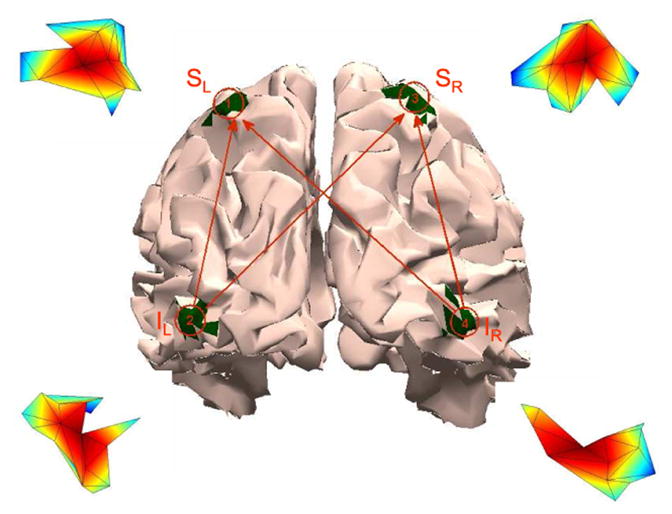
Inferior occipital gyrii (I_L and I_R) and superior parietal lobules (S_L and S_R) are shown in green on a rear view of the brain. The line drawing superimposed on the brain illustrates the causal influences simulated in Examples 3 and 4 while the insets near each ROI depict the simulated spatial activity distribution

$${\mathbf{y}}_n=\sum _{i=1}^Q{\mathbf{h}}^i{\alpha }_n^i$$ (10)

where hⁱ is the leadfield for a dipole at the i^th grid location and ${\alpha }_n^i$ is the corresponding current source density. Rewrite this expression in matrix notation as

$${\mathbf{y}}_n=\mathbf{H}{\mathit{\alpha }}_n$$ (11)

where H = [h¹, h², …, h^Q] is the collection of leadfields in the ROI and ${\mathit{\alpha }}_n={[{\alpha }_n^1,{\alpha }_n^2,\dots ,{\alpha }_n^Q]}^T$ describes the current source spatial distribution over Ω.

At typical SNR and values of Q we cannot see all Q spatial degrees of freedom in the measurement y_n because of ill-conditioning in the forward physics. That is, in practice H is a low-rank matrix. Let the singular value decomposition of H be UΣV^T and represent the K largest singular values and corresponding singular vectors of H using the matrices U^K, Σ^K and V^K, where U^K and V^K contain the first K columns of U and V, respectively, and Σ^K is the K by K upper left block of Σ. Hence, a rank K approximation to H is H ≈ U^KΣ^KV^KT. Limpiti, et al. [25] found that H was well modeled as rank 4 or less for ROIs as big as 590 mm² and termed the columns of U^K cortical patch bases. We define the L by K matrix C = U^KΣ^K and K by 1 vector λ_n = V^KT α_n to approximate Eq. (11) in terms of the K degrees of freedom in the measurement as

$${\mathbf{y}}_n=\mathbf{C}{\mathbf{\lambda }}_n.$$ (12)

Thus, although an ROI may involve a spatial sampling of several hundred grid points, a very small number of these degrees of freedom are visible in the measured data. The visible spatial degrees of freedom are represented by the K entries in λ_n. The current source density distribution α_n associated with Eq. (12) is of the form α_n = V^Kλ_n. This follows from V^KT V^K = I and Cλ_n ≈ Hα_n. Hence, the left singular vectors in V^K are a basis for spatial patterns α_n that are measurable at the scalp. Note that Eq. (12) also applies to dipolar source models with unknown moment orientation. In this case C is the L by 3 leadfield matrix for the dipole location and λ_n is the dipole moment.

In general the spatial pattern within the i^th ROI varies with time, as indicated by the notation ${\mathit{\alpha }}_n^i$ and ${\mathbf{\lambda }}_n^i$. The EM algorithm presented in Section IV is applicable to this case, however, for simplicity we assume here that the spatial pattern does not vary with time. That is, ${\mathbf{\lambda }}_n^i={\mathbf{\lambda }}^i{x}_n^i$ where λⁱ describes the pattern and $x_n^i$ the amplitude as a function of time. In the case of a dipolar source model, this implies the moment orientation is fixed (λⁱ) while the amplitude $x_n^i$ varies with time.

The measured signal is expressed as a sum of the activity due to each ROI plus a noise term v_n,j that accounts for measurement noise and unmodeled source activity. Let the activity due to the i^th ROI be represented as ${\mathbf{C}}^i{\mathbf{\lambda }}^i{x}_{n,j}^i$ and write

$${\mathbf{y}}_{n,j}=\sum _{i=1}^M{\mathbf{C}}^i{\mathbf{\lambda }}^i{\mathbf{x}}_{n,j}^i+{\mathbf{v}}_{n,j}.$$ (13)

The ROIs are assumed known but the spatial patterns are unknown, so Cⁱ is known but λⁱ is unknown. We rewrite Eq. (13) in terms of x_n,j as

$${\mathbf{y}}_{n,j}=\mathbf{C}\mathbf{\Lambda }{\mathbf{x}}_{n,j}+{\mathbf{v}}_{n,j}$$ (14)

where C = [C¹, C², …, C^M] is now an L by MK matrix and

$$\mathbf{\Lambda }=\left[\begin{array}{cccc}{\mathbf{\lambda }}^1& 0& 0& 0\\ 0& {\mathbf{\lambda }}^2& 0& ⋮\\ ⋮& 0& \ddots & 0\\ 0& \cdots & 0& {\mathbf{\lambda }}^M\end{array}\right]$$ (15)

is MK by M. Note that it is not necessary to assume each ROI uses the same number of spatial degrees of freedom K; we have done so for notational convenience. We assume the noise v_n,j is multivariate Gaussian distributed with mean zero and covariance matrix R and is independent across samples and epochs.

C. The State-Space Model

The observation equation (14) and MVAR model (9) combine to provide a state-space representation for the measured data

$$\begin{array}{l}{\mathbf{x}}_{n,j}=\mathbf{A}{\mathbf{z}}_{n-1,j}+{\mathbf{w}}_{n,j}\\ {\mathbf{y}}_{n,j}=\mathbf{C}\mathbf{\Lambda }{\mathbf{x}}_{n,j}+{\mathbf{v}}_{n,j}\end{array}$$ (16)

where w_n,j ~ N(0, Q) and v_n,j ~ N(0, R). We assume C is known, but A, Q, x_n,j, Λ, R are unknown. Furthermore, z_0,j ~ N (μ₀, Σ₀) with μ₀ and Σ₀ unknown.

The question of uniqueness is addressed by considering whether y_n,j is invariant to any transformation of the state x_n,j. If transformations of the state do not affect y_n,j, then there are many models capable of describing identical measured data. Let x̃_n,j = Ψx_n,j where Ψ is a nonsingular state transformation. Assuming C is full rank, uniqueness of y_n,j with respect to Ψ requires that there is no valid Λ̃ for which Λx_n,j = Λ̃x̃_n,j. That is, the model is unique if and only if Λ = Λ̃Ψ implies the matrix Ψ = I.

First note that both Λ and Λ̃ must have the block structure in Eq. (15). This implies Ψ must be a block diagonal matrix, which implies λⁱ = λ̃ⁱψⁱ where ψⁱ is the i^th diagonal element of Ψ. Hence the model of Eq. (16) is not unique with respect to the magnitude and sign of the cortical signals $x_{n,j}^i$; an increase in the magnitude of $x_{n,j}^i$ is offset by a decrease in λⁱ. The magnitude ambiguity is eliminated by requiring λ^iT λⁱ = 1, that is, by normalizing the cortical signals $x_{n,j}^i$ to be proportional to the corresponding cortical current density. The sign ambiguity implies λⁱ = − λ̃ⁱ and $x_{n,j}^i=-{\stackrel{\sim }{x}}_{n,j}^i$ produce equivalent measurements. This sign ambiguity leads to sign ambiguities in the entries of A; however such ambiguities do not alter the connectivity structure of the MVAR model and will not be considered further.

IV. An EM Algorithm for Maximum Likelihood Estimation of Model Parameters

ML estimates have the desirable properties of being unbiased and attaining the Cramer-Rao lower bound on variance in the asymptotic case of increasing data length/epochs [16]. EM algorithms are used in a variety of incomplete-data problems when closed-form expressions for ML estimates are not available. They monotonically increase likelihood at each iteration and are guaranteed to converge to a maximum of the likelihood surface [26]. EM algorithms have been developed for state-space models by Shumway and Stoffer [21] and others. Our algorithm differs from previously proposed approaches because the state x_n,j is observed through the product of a known matrix C and unknown, structured matrix Λ.

The EM algorithm computes the ML estimates of Θ = {A, Q, R, μ₀, Σ₀, Λ} for the state-space model described in Eq. (16). We assume N time samples are available in each of J epochs. Let {Y, X} denote the so-called complete data, where Y = {y_1,1, …, y_N,1, …, y_1,J, …, y_N,J} is the observed data and X = {x_1,1, …, x_N,1, …, x_1,J, …, x_N,J} is the hidden data. The complete data likelihood function can be written in the form

$$p(\mathbf{Y},\mathbf{X};\mathbf{\Theta })=\prod _{j=1}^{J}p({\mathbf{z}}_{0,j})\prod _{n=1}^{N}p({\mathbf{y}}_{n,j}\mid {\mathbf{x}}_{n,j})p({\mathbf{x}}_{n,j}\mid {\mathbf{z}}_{n-1,j}).$$ (17)

The probability densities p(z_0,j), p(y_n,j|x_n,j) and p(x_n,j|z_n−1,j) are given by the Gaussian distributions N(μ₀, Σ₀), N(CΛx_n,j, R) and N(Az_n−1,j, Q), respectively.

The EM algorithm iteratively maximizes the conditional expectation of the log-likelihood of the complete data using a series of two steps in each iteration. In the first step, known as the expectation step (E-step), the expectation of the log likelihood of the complete data

$$q(\mathbf{\Theta }\mid {\mathbf{\Theta }}^r)=E\{logp(\mathbf{Y},\mathbf{X};\mathbf{\Theta })\mid \mathbf{Y}\mid {\mathbf{\Theta }}^r\}$$ (18)

is computed conditioned on the measured data and the estimated parameters at the previous iteration, denoted as ${\mathbf{\Theta }}^r=\{{\mathbf{A}}^r,{\mathbf{Q}}^r,{\mathbf{R}}^r,{\mathit{\mu }}_0^r,{\mathbf{\sum }}_0^r,{\mathbf{\Lambda }}^r\}$. The second step, known as the maximization step (M-step), finds new parameter estimates Θ^r+1 by maximizing q(Θ|Θ^r) with respect to Θ. These two steps are repeated until the likelihood of the observed data converges to a maximum value.

The log likelihood of the observed data is proportional to

$$logp(\mathbf{Y}\mid {\mathbf{\Theta }}^r)=-\frac{1}{2}\sum _{j=1}^J\sum _{n=1}^{N}log\mid {\mathbf{P}}_{e_{n,j}}({\mathbf{\Theta }}^r)\mid +{\mathbf{e}}_{n,j}^T({\mathbf{\Theta }}^r){\mathbf{P}}_{e_{n,j}}^{-1}({\mathbf{\Theta }}^r){\mathbf{e}}_{n,j}({\mathbf{\Theta }}^r)$$ (19)

where e_n,j(Θ^r) is the prediction error and P_en,j(Θ^r) is the error covariance matrix, both of which can be obtained from the Kalman filter [27] as described in [28]. The EM iterations are terminated when the relative change in the likelihood of Eq. (19) drops below 10⁻⁵. Since the EM algorithm is guaranteed to converge to a local maximum of the log likelihood function [26], we start the algorithm from multiple randomized initial conditions and select the solution with the largest likelihood. Additional details of the EM algorithm and the choice of initial conditions are given in the Appendix.

V. Cortical Connectivity via Conditional Granger Causality

Multiple measures of connectivity between cortical signals can be obtained from the MVAR model parameters including directed transfer function [9] and partial directed coherence [10]. In this manuscript we employ the conditional Granger causality metric introduced by Geweke [8] to illustrate the merits of our state-space approach. Consider three vector time-series u_n, v_n and z_n and define the past of each time series as U_n−1 = {u₁, u₂, …, u_n−1}, V_n−1 = {v₁, v₂, …, v_n−1} and Z_n−1 = {z₁, z₂, …, z_n−1} respectively. The Granger causality from v_n to u_n conditioned on z_n is given by [8]

$$F_{\mathbf{V}\to \mathbf{U}\mid \mathbf{Z}}=log\frac{\mid {\mathbf{\sum }}_1\mid }{\mid {\mathbf{\sum }}_2\mid }$$ (20)

where Σ₁ is the error covariance matrix for predicting u_n using both U_n−1 and Z_n−1, and Σ₂ is the error covariance matrix for predicting u_n using U_n−1, V_n−1 and Z_n−1. It is easy to show |Σ₂| ≤ |Σ₁| [29]. This implies F_V→U|Z ≥ 0 with F_V→U|Z increasing as the ability of V_n−1 to improve the prediction of u_n increases. Note that F_V→U|Z differentiates the direct influence of V_n−1 on u_n from the indirect influence of V_n−1 mediated through Z_n−1.

In the context of MVAR modeling, the error covariance matrix Σ₁ is replaced by Q₁, the error covariance matrix based on an MVAR model using u_n and z_n, and Σ₂ is replaced by Q₂, the error covariance matrix for an MVAR model employing u_n, z_n and v_n. This requires estimating two MVAR models and can produce negative values of F_V→U|Z due to estimation errors [30]. Furthermore, the potential for F_V→U|Z to be negative is exacerbated with the state-space formulation when two distinct models are estimated because the cortical signals are measured in the presence of observation noise and the observation noise covariance matrix is estimated separately for each model. Differences in the two MVAR models may be obscured by changes in the estimated noise covariance matrix. Chen, et al., [30] introduce a partitioned matrix approach for computing F_V→U|Z based on one MVAR model that is guaranteed to produce a nonnegative metric and we employ this approach here. The partitioned matrix approach is also beneficial with our state-space formulation as it avoids the computational cost of estimating multiple MVAR models.

VI. Simulation Results

Four examples based on simulated data are presented to illustrate the effectiveness and performance attributes of our state-space approach when the true connectivity is known. We compare the results of our state-space approach to the two-stage nulling beamformer (NBF) approach proposed by Hui, et al. in [15]. The NBF is based on same singular vectors used to construct the Cⁱ in (13), so equivalent source models are employed. In each example we use N = 200 samples and J = 15 epochs and run the example over 100 different signal and noise realizations to estimate the mean and variance of the Granger causality metric. The observation equation assumes a 56-channel EEG system. Spatially white observation noise is simulated and we define SNR as

$$\frac{\text{tr}\{{\sum }_{j=1}^J{\sum }_{n=1}^N{\sum }_{i=1}^M({\mathbf{H}}^i{\mathit{\alpha }}_{n,j}^i){({\mathbf{H}}^i{\mathit{\alpha }}_{n,j}^i)}^T\}}{\text{tr}\{{\sum }_{j=1}^J{\sum }_{n=1}^N({\mathbf{v}}_{n,j}){({\mathbf{v}}_{n,j})}^T\}}$$

where Hⁱ is the collection of leadfields in the i^th ROI and ${\mathit{\alpha }}_{n,j}^i={\mathit{\alpha }}^i{x}_{n,j}^i$ is the corresponding spatial-temporal source activity. Example 1 presents a scenario to support the analysis given in Section II while Example 2 to 4 introduce various modeling errors for studying the robustness of our approach.

Example 1: Two ROI connectivity

We assume two dipolar sources with known moments in the left hemisphere as shown by the markers in Fig. 1, and simulate cortical signals using the following first order MVAR model:

$$\begin{array}{l}{x}_{n,j}^1=0.6x_{n-1,j}^1+w_{n,j}^1\\ x_{n,j}^2=-0.2x_{n-1,j}^1+0.7x_{n-1,j}^2+w_{n,j}^2.\end{array}$$ (21)

Fig. 1.

Dipolar source locations for Example 1 (the black source is hidden in a sulcus). The blue shaded region depicts all source locations that have forward model angles equal or exceeding cos θ = 0.8 with respect to the red source.

The covariance matrix Q used to simulate the data is diagonal with Q¹¹ = 0.6 and Q²² = 0.2. Note that this model involves causal influence from source 1 to source 2, and no influence in the reverse direction. Both the EM algorithm and NBF approach are used to estimate the MVAR parameters to support the analysis in Section II.

Fig. 2 depicts the true and estimated MVAR model coefficients A²¹ and A¹² and the Granger causality between the dipoles marked in red and green in Fig. 1 as a function of SNR. Here the angle between the source forward models (see Section II) is cos θ = 0.8. The EM approach produces unbiased estimates of MVAR model coefficients and Granger causality across the entire range of SNRs. In contrast, the bias in the NBF increases significantly as the SNR decreases. In this example the EM approach obtains performance comparable to the NBF approach with over 15 dB less SNR.

Fig. 2.

EM and NBF approach performance as a function of SNR estimated over 100 runs. Error bars denote one standard deviation. (a) MVAR cross coupling coefficients A¹² and A²¹. (b) Granger causality metric from source 1 to source 2 and source 2 to source 1.

The influence of the angle between the source forward models on the EM and NBF approaches is depicted in Fig. 3 assuming SNR = −5 dB. The angle cos θ = 0.2 is obtained using sources at the red and black (arrow in Fig. 1) markers, cos θ = 0.5 is obtained using sources at the red and magenta markers, and cos θ = 0.8 is obtained using sources at red and green markers in Fig. 1. Angles cos θ ≥ 0.8 with respect to the red source are not unusual; the blue shaded regions in Fig. 1 depict all sources that satisfy cos θ ≥ 0.8. The performance of the EM approach is insensitive to the angle between the forward models, while, as predicted in Section II, the NBF approach performance degrades significantly as the angle decreases.

Fig. 3.

EM and NBF approach performance as a function of the angle between source forward models estimated over 100 runs at SNR = −5 dB. Error bars denote one standard deviation. (a) MVAR cross coupling coefficients A¹² and A²¹. (b) Granger causality metric from source 1 to source 2 and source 2 to source 1.

Example 2: Two ROI Connectivity with Interference

In this example we simulate two spatially distributed sources (ROI 1 and ROI 2) whose cortical signals follow the MVAR model in Eq. (21). The activity simulated in each ROI has a raised cosine distribution with 10 mm geodesic radius. A third, independent spatially distributed and temporally random source is introduced as an interferer. The contributions from the i^th ROI are simulated using Eq. (11) where ${\mathit{\alpha }}_{n,j}^i={\mathit{\alpha }}^i{x}_{n,j}^i$. Here αⁱ implements the raised cosine distribution and $x_{n,j}^i$ is the cortical signal from the i^th ROI at time n and epoch j. The interfering source is not modeled in the state equation (Eq. (9)) when the simulated data is processed, and thus contributes to the observation noise v_n,j in Eq. (14). The two sources of interest are represented in the observation equation (Eq. (14)) by designing C assuming only the ROI extent is known and using K = 3 basis vectors to represent each ROI. The SNR in the absence of the interfering source is 5 dB. Fig. 4 shows source and interferer locations for two cases: where the angle between source 1 and interferer is cos θ = 0.5, and where the interferer and source 1 satisfy cos θ = 0.8. The interferer and source 2 are at identical locations in each scenario. When cos θ = 0.5 the interferer and source 1 are well separated.

Fig. 4.

Two-source and interferer scenarios for Example 2. The green patch is the interferer while the purple patch is source 2. The red and blue patches depict the locations of source 1 for two different scenarios.

Fig. 5 compares the estimated and true Granger causality from source 1 to source 2 as a function of the signal to interference (SIR) level for both scenarios. The results for Granger causality from source 2 to source 1 are close to 0 in both EM and NBF approaches and are not shown in Fig. 5. The SIR is defined as

Fig. 5.

Estimated and true Granger causality from source 1 to source 2 for a simulated two-node network in the presence of an interfering source as a function of SIR and the angle between the interferer and source 1 forward models at SNR = 5 dB. Error bars denote one standard deviation.

$$\frac{\text{tr}\{{\sum }_{j=1}^J{\sum }_{n=1}^N{\sum }_{i=1}^2({\mathbf{H}}^i{\mathit{\alpha }}_{n,j}^i){({\mathbf{H}}^i{\mathit{\alpha }}_{n,j}^i)}^T\}}{\text{tr}\{{\sum }_{j=1}^J{\sum }_{n=1}^N(\stackrel{\sim }{\mathbf{H}}{\stackrel{\sim }{\mathit{\alpha }}}_{n,j}){(\stackrel{\sim }{\mathbf{H}}{\stackrel{\sim }{\mathit{\alpha }}}_{n,j})}^T\}}$$

The matrix H̃ is the collection of leadfields in the interfering cortical patch and α̃_n,j is the spatial-temporal activity of cortical interferer. SIR = ∞ implies the interferer is not present, while SIR = −10 dB implies the interferer power is 10 times as large as the source power in the measured data. The results indicate that the presence of the interferer causes only a slight shift in the mean estimated Granger causality from source 1 to source 2 that is nearly independent of the interferer strength. The EM approach is robust to unmodeled, independent source activity because such activity is represented in the state-space model by the observation noise. NBF is also robust to interfering source activity because output power is minimized, although it exhibits some sensitivity to the angle between source 1 and the interferer.

Example 3: Four Spatially Distributed Sources

This example is inspired by the properties of the human subject example presented in Section VII. The four ROIs are the inferior occipital gyrii (IOG) and the superior parietal lobules (SPL) in each hemisphere as illustrated in Fig. 6. The activity simulated in each ROI has a raised cosine distribution with 10 mm geodesic radius as shown by the insets in Fig. 6. A P = 4 order MVAR model is simulated to generate the back-to-front causal influences depicted by the line drawing superimposed on the cortical surface in Fig. 6.

The matrix C in the observation equation (Eq. (14)) is designed assuming the ROI extent is known, but the spatial distribution of activity within each ROI is unknown as described in Section III.B. The results obtained using K = 2 and K = 3 singular vectors for each ROI at SNR = 5 dB are depicted in Fig. 7. Note that as K increases, the number of spatial degrees of freedom estimated and the ability to represent spatial detail for each ROI increases. Hence we observe that at high SNR the K = 3 based solution provides better quality estimates of Granger causality than K = 2. At lower SNR (not shown) the K = 2 based solution results in less bias than K = 3 because the spatial detail is less visible at lower SNR and the additional spatial degrees of freedom associated with K = 3 are more difficult to estimate. The NBF significantly underestimates Granger causality.

Fig. 7.

Estimated and true conditional Granger causality for the simulated four-node network of Example 3 as depicted in Fig. 6 at SNR = 5 dB. The observation equation (Eq. 14) is designed using either K = 2 or K = 3 basis vectors for each ROI. Error bars denote one standard deviation.

Example 4: Four ROIs with Spatial Mismatch

This example uses two MVAR models with order P = 4 corresponding to the scenario in Fig. 6 to explore the effects of errors in assumed ROI location and extent. Three different observation models are considered. The first assumes the true ROIs (10 mm geodesic radius) are used in the observation equation (Eq. (14)). In the second case the centers of the assumed ROIs used in the observation equation are 10 mm from the true centers. The third case assumes the ROI centers are 10 mm from the true centers and the geodesic radius of each ROI is 20 mm instead of the true value of 10 mm. Each ROI is represented in the observation equation using K = 3 singular vectors. The results are depicted in Fig. 8 for SNR = 5 dB. Note that ROI location mismatch and location/size mismatch result in relatively small errors in the estimated Granger causality relative to the case of no mismatch for the EM approach. NBF significantly underestimates Granger causality and exhibits greater sensitivity to mismatch.

Fig. 8.

Estimated and true conditional Granger causality corresponding to the simulated four-node network depicted in Fig. 6 with ROI mismatch at SNR = 5 dB. Error bars denote one standard deviation.

VII. Application To Real EEG Data

We apply the EM algorithm to 56 channels of EEG data collected from three healthy subjects passively watching a 30-minute portion of an engrossing movie (The Good, The Bad, and The Ugly). The data were zero-phase filtered using a Chebyshev type II filter with passband 1Hz - 20Hz and then down sampled to a 62.5 Hz sampling rate. Three artifact free segments were selected from EEG recordings for each subject to gauge consistency of the estimated connectivity. For Subject 1 each segment consists of one contiguous 16-sec epoch, while for Subjects 2 and 3 each segment consists of four 3-sec epochs. Connectivity between IOG and SPL regions in both hemispheres is evaluated because these regions are likely to be activated by visual simulation [31], [32]. Fig. 6 depicts these four regions on a cortical surface reconstruction of the average brain from the Montreal Neurological Institute (MNI). Each of the four ROIs is modeled using K = 3 singular vectors. Forward models for the dipoles in each ROI are computed within the Geosource software package (EGI, Eugene, OR) using a four-shell spherical head model with locations derived from the MNI probabilistic atlas. Dipoles are constrained to 7mm cortical voxels of the average MNI brain and consist of three orthogonal source orientations (xyz). The MVAR model order P is selected based on the Bayesian information criterion (BIC) [33]

$$\mathit{BIC}(p)=-2logp(\mathbf{Y}\mid {\mathbf{\Theta }}_p)+{\varphi }_{p}log(T)$$ (22)

where log p(Y|Θ_p) is the maximum observed data log-likelihood defined in Eq. (19), ϕ_p is the number of free parameters estimated by EM and T = N × J is the total number of samples. The BIC curves vary; however, P = 12 is the exact or near minimum BIC in each subject.

An order P = 12 MVAR model is estimated using the EM algorithm and the conditional Granger causality metric between the two IOG and SPL regions is computed. Fig. 9 depicts the results of processing each segment for Subject 1. Only significant conditional Granger causality values are shown. We determined a significance threshold for each connection using random temporal permutation of the measured data to destroy cortical interactions. One hundred random permutations of the data over time and epochs for each subject/segment are generated using MATLAB’s “randperm” command and an order P = 12 MVAR model is fit to each permutation using the EM algorithm to obtain a histogram of conditional Granger causality under the hypothesis that the interactions are zero. Significance thresholds are determined such that only 5% of the permuted cases exceed the threshold. Connection S_L → I_R is not significant in all three segments for Subject 1. In Subject 2 and 3 all non-homologous connections are significant for all three segments.

Fig. 9.

Subject 1 conditional Granger causality metrics estimated during movie viewing for three different segments of data.

We assess the consistency of the estimated conditional Granger causality values across the three independent segments in all three subjects by computing the coefficient of variation (CV). CV is the ratio of the sample standard deviation to the sample mean expressed as a percentage [34]. Hence, a CV of 0% indicates the three values are identical, while a CV of 100% indicates the sample standard deviation is equal to the mean. For example, the CV for I_L → S_L in Fig. 9 is 12.5% while S_R → I_R is 29.4%. A histogram of CV values for the 23 significant non-homologous connections in all three subjects is shown in Fig. 10. Fifteen of the 23 CV values are less than 20% and the maximum CV is 34.4%. This indicates general consistency in the estimated conditional Granger causality metric across different segments of data.

Fig. 10.

Histogram of the coefficient of variation for non-homologous connections in all three subjects.

The results reveal general patterns of consistency between the three segments for each subject. The true connectivity pattern for each subject is unknown and likely varies some between segments. The consistency of the estimates between segments and significance relative to that of temporally permuted data suggest that this approach is identifying genuine cortical interactions.

VIII. Discussion

The state-space formulation of Eq. (16) integrates the MVAR cortical connectivity model with the EEG measurement physics and explicitly accounts for the presence of noise in the measured data. The presence of noise is not explicitly addressed when estimating MVAR parameters via two-stage approaches that attempt to first estimate cortical signals and then fit an MVAR model to the estimated cortical signals. Our analysis reveals that noise in the estimated cortical signals from two-stage approaches leads to biased MVAR parameter estimates, and that the effect of the noise depends strongly on the cosine of the angle between the forward models associated with different sources. In contrast, the EM algorithm provides a means for obtaining ML estimates of the MVAR model parameters in the state-space formulation. ML methods are known to be asymptotically unbiased, and thus, given sufficient data, our EM approach is expected to yield unbiased MVAR model parameter estimates.

Simulated examples support our analysis of two-stage approaches. Bias in estimated Granger causality is evident at all but the highest SNRs and this bias depends on the similarity of the forward models associated with different cortical sources. Simulations also show that our EM approach yields unbiased Granger causality estimates at significantly lower SNRs and is relatively insensitive to varying similarity between forward models. The NBF is sensitive to the similarity between forward models and the performance degrades significantly as SNR decreases. The NBF significantly underestimates Granger causality in the four ROI examples, even at a relatively high SNR of 5 dB. The robustness of our state-space approach to noise is a significant advantage given the relatively low SNR of typical EEG data.

Explicitly modeling noise with unknown spatial covariance also endows our approach with robustness to artifacts and brain activity that is not from an ROI of interest, as shown in Fig. 5. The estimated Granger causality is relatively insensitive to the power of a spatially distributed interfering source for two different source/interferer configurations.

The observation model of Eq. (14) describes extended cortical sources with unknown spatial activity distribution in a very parsimonious fashion by only representing the components of the spatial activity that are measurable via EEG physics. This significantly reduces the number of unknown parameters that must be estimated compared to approaches that tessellate the cortical ROIs with dipoles and estimate the strength of each dipole. At high SNR fine structure in the spatial activity distribution is more visible and a larger number of bases are recommended. At low SNR the fine structure of the cortical source spatial distributions is buried in the noise and fewer bases should be used since the estimated coefficients of higher order bases will be dominated by noise. These conclusions are supported by the results given in Fig. 7. The number of bases appropriate for a given source is also proportional to the spatial extent of the ROI. Given our experience with these bases in this and source localization applications [25], [35], we anticipate that between two and five bases per ROI will be appropriate in most MVAR modeling applications.

Our source model also provides a principled way of associating a single time series with a ROI while allowing the spatial activity distribution within the ROI to be unknown. In contrast, the two-stage approach of [12] averages magnitudes of each dipole in the ROI – a nonlinear step that may alter the estimated cortical interactions, while the NBF approach of [15] can only return a single time series for an ROI. It is possible to employ conditional Granger causality to estimate connectivity when more than one time series is associated with each ROI. Use of a single time series implies that the spatial activity distribution is constant, i.e., it varies only in amplitude. Our approach is easily extended to represent time varying spatial activity patterns by using a second time series for a ROI. In this case the spatial activity in the ROI is the sum of the patterns associated with the first and second time series and this sum varies with time. We have focused here on the constant spatial pattern case because reliable estimation of time-varying spatial patterns is likely to require higher SNR and fairly large ROIs to compensate for the additional complexity in the spatial and MVAR models.

The requirement that C is full rank ultimately determines the maximum number and locations of ROIs that can be studied. Linear dependence between the columns of C implies that activity in one ROI cannot be distinguished from activity in another ROI. In practice, the noise covariance matrix and singular values of C determine the number and locations of ROIs for which it is reasonable to estimate an MVAR model. since the singular values of C represent the strength with which the corresponding cortical signal component can be measured. We recommend that users evaluate the singular values of C and exercise caution with scenarios involving relatively small singular values. Similar limitations apply to the NBF.

Use of spatial bases with unknown coefficients (the λⁱ in Eq. (14)) for describing source activity provides some measure of robustness to uncertainty in the source forward models, e.g., due to use of a template brain, errors in assumed source locations, and various errors in cortical surface extraction, coregistration, and electrical properties. The robustness results because the unknown coefficients are chosen to provide the best fit to the true spatial distribution of the source. These conclusions are supported by the results shown in Fig. 8 –the connectivity estimates are not significantly affected by errors in the ROI locations and extent. Note, however, that this implies care must be exercised when estimating connectivity between ROIs that have very similar (nearly linearly dependent) bases, because the coefficients for each ROI may extract the identical (or very similar) underlying source activity.

We have assumed the locations of the cortical sources of interest are known, as is typical for previously proposed MVAR modeling approaches. For example, Hui, et al., [15] also assume ROIs are known. Babiloni, et al. [12] and Astolfi, et al. [13], [14] select ROIs based on anatomy, as we have done in Section VII. Ding, et al. [11] use a source localization technique to identify ROIs. Note that use of source localization to identify ROIs does not eliminate the advantages of the state-space formulation relative to two-stage connectivity estimation methods. The disadvantage of two-stage methods lies in decoupling the estimation of cortical signals from estimation of MVAR model parameters.

Clear validation of cortical connectivity estimation algorithms using human data is very difficult because the true connectivity is rarely known to reasonable precision. Hence, we have assessed consistency of connectivity estimates across three distinct segments of data in three subjects. All three segments lead to either significant (23/24) or insignificant (1/24) connectivity estimates using thresholds obtained after connectivity is destroyed via random temporal shuffling of the data. Second, the patterns in estimated conditional Granger causality for different connections within each subject are consistent across segments. For example, Subject 1 (Fig. 9) shows I_L → S_L as the strongest connection in each segment, while S_L → I_L and I_L → S_R are consistently of moderate strength and S_R → I_L and I_R → S_L are consistently the weakest significant connections. Third, the CV for each connection in each subject is relatively small. The maximum CV is 34.4% and 15 of the 23 significant connections have CV’s less than 20%. This high level of consistency within each subject across independent data segments strongly suggests that our estimated models are reflecting underlying physiological interactions and not noise. The movie viewing experimental paradigm was not designed to assess consistency between subjects; this will be the subject of future research.

Although the focus of this paper is EEG, it is straightforward to apply the state-space formulation and EM algorithm to MEG data. The only modification to the procedure is that the observation matrix C in Eq. (14) is designed using MEG forward models.

Biographies

Patrick Cheung Bing Leung Patrick Cheung (S’00-M’02) received the B.A.Sc. degree with honors in computer engineering from the University of British Columbia, Vancouver, BC, Canada, in 2000 and the M.S. degree in electrical engineering from Virginia Tech, Blacksburg, VA, in 2002. He is currently working towards the Ph.D. degree at the University of Wisconsin, Madison.

From 2002 to 2006, he worked as a wireless system engineer specialized in radio algorithm development and digital signal processing at Nortel Networks in Canada. His research interests include system identification, statistical signal processing and time series analysis for biomedical applications.

Mr. Cheung received a Natural Sciences and Engineering Research Council of Canada (NSERC) Postgraduate Scholarship for 2008–2010.

Brady Riedner Brady Alexander Riedner received a B.S. degree in philosophy and history from the University of Wisconsin, Madison in 1996. Since 2005, he has been working towards a Ph.D. in the Neuroscience Training Program at that institution.

His research primarily involves using high-density EEG to study sleep. Particularly, he has done considerable work characterizing the spatiotemporal dynamics of EEG sleep slow waves.

Mr. Riedner was awarded the Clinical Neuroengineering Training Program award in 2006.

Giulio Tononi Giulio Tononi is a psychiatrist and neuroscientist who has held faculty positions in Pisa, New York, San Diego and Madison, Wisconsin, where he is Professor of Psychiatry. Dr. Tononi and collaborators have pioneered several complementary approaches to study sleep. These include genomics, proteomics, fruit fly models, rodent models employing multiunit/local field potential recordings in behaving animals, in vivo voltammetry and microscopy, high-density EEG recordings and transcranial magnetic stimulation in humans, and large-scale computer models of sleep and wakefulness. This research has led to a comprehensive hypothesis on the function of sleep, the synaptic homeostasis hypothesis. According to the hypothesis, wakefulness leads to a net increase in synaptic strength, and sleep is necessary to reestablish synaptic homeostasis. The hypothesis has implications for understanding the effects of sleep deprivation and for developing novel diagnostic and therapeutic approaches to sleep disorders and neuropsychiatric disorders. Another focus of Dr. Tononi’s work is the integrated information theory of consciousness: a scientific theory of what consciousness is, how it can be measured, how it is realized in the brain and, of course, why it fades when we fall into dreamless sleep and returns when we dream. The theory is being tested with neuroimaging, transcranial magnetic stimulation, and computer models. In 2005, Dr. Tononi received the NIH Director’s Pioneer Award for his work on sleep mechanism and function, and in 2008 he was made the David P. White Chair in Sleep Medicine and is a Distinguished Chair in Consciousness Science.

Barry Van Veen Barry D. Van Veen (S’81-M’86-SM’97-F’02) was born in Green Bay, WI. He received the B.S. degree from Michigan Technological University in 1983 and the Ph.D. degree from the University of Colorado in 1986, both in electrical engineering. He was an ONR Fellow while working on the Ph.D. degree.

In the spring of 1987 he was with the Department of Electrical and Computer Engineering at the University of Colorado-Boulder. Since August of 1987 he has been with the Department of Electrical and Computer Engineering at the University of Wisconsin-Madison and currently holds the rank of Professor. His research interests include signal processing for sensor arrays and biomedical applications of signal processing.

Dr. Van Veen was a recipient of a 1989 Presidential Young Investigator Award from the National Science Foundation and a 1990 IEEE Signal Processing Society Paper Award. He served as an associate editor for the IEEE Transactions on Signal Processing and on the IEEE Signal Processing Society’s Statistical Signal and Array Processing Technical Committee and the Sensor Array and Multichannel Technical Committee. He is a Fellow of the IEEE and received the Holdridge Teaching Excellence Award from the ECE Department at the University of Wisconsin in 1997. He coauthored “Signals and Systems,” (1st Ed. 1999, 2nd Ed., 2003 Wiley) with Simon Haykin.

Appendix

EM Algorithm: E-step and M-step

Following [21], we expand Eq. (18) and write the result of the E-step as

$$q(\mathbf{\Theta }\mid {\mathbf{\Theta }}^r)=E\{logp(\mathbf{Y},\mathbf{X};\mathbf{\Theta })\mid \mathbf{Y},{\mathbf{\Theta }}^r\}\propto -\frac{J}{2}log\mid {\mathbf{\sum }}_0\mid -\frac{1}{2}\text{tr}\left\{{\mathbf{\sum }}_0^{-1}\sum _{j=1}^J({\mathbf{P}}_{0\mid N,j}+({\mathbf{z}}_{0\mid N,j}-{\mu }_0){({\mathbf{z}}_{0\mid N,j}-{\mu }_0)}^T)\right\}-\frac{JN}{2}log\mid \mathbf{Q}\mid -\frac{1}{2}\text{tr}\left\{{\mathbf{Q}}^{-1}(\mathbf{D}-\mathbf{E}{\mathbf{A}}^T-\mathbf{A}{\mathbf{E}}^T+\mathbf{AF}{\mathbf{A}}^T)\right\}-\frac{JN}{2}log\mid \mathbf{R}\mid -\frac{1}{2}\text{tr}\left\{{\mathbf{R}}^{-1}\left[\sum _{j=1}^J\sum _{n=1}^N({\mathbf{y}}_{n,j}-\mathbf{C}\mathbf{\Lambda }{\mathbf{x}}_{n\mid N,j})\times {({\mathbf{y}}_{n,j}-\mathbf{C}\mathbf{\Lambda }{\mathbf{x}}_{n\mid N,j})}^T+\mathbf{C}\mathbf{\Lambda }{\mathbf{P}}_{n\mid N,j}{(\mathbf{C}\mathbf{\Lambda })}^T\right]\right\}$$ (23)

where

$$\mathbf{D}=\sum _{j=1}^J\sum _{n=1}^N{\mathbf{P}}_{n\mid N,j}+{\mathbf{x}}_{n\mid N,j}{\mathbf{x}}_{n\mid N,j}^T$$ (24)

$$\mathbf{E}=\sum _{j=1}^J\sum _{n=1}^N{\mathbf{P}}_{n,n-1\mid N,j}+{\mathbf{x}}_{n\mid N,j}{\mathbf{z}}_{n-1\mid N,j}^T$$ (25)

$$\mathbf{F}=\sum _{j=1}^J\sum _{n=1}^N{\mathbf{P}}_{n-1\mid N,j}+{\mathbf{z}}_{n-1\mid N,j}{\mathbf{z}}_{n-1\mid N,j}^T$$ (26)

and the quantities

$${\mathbf{x}}_{n\mid N,j}=E\{{\mathbf{x}}_{n,j}\mid \mathbf{Y},{\mathbf{\Theta }}^r\}$$ (27)

$${\mathbf{z}}_{n-1\mid N,j}=E\{{\mathbf{z}}_{n-1,j}\mid \mathbf{Y},{\mathbf{\Theta }}^r\}$$ (28)

$${\mathbf{P}}_{n\mid N,j}=E\{({\mathbf{x}}_{n,j}-{\mathbf{x}}_{n\mid N,j})\times {({\mathbf{x}}_{n,j}-{\mathbf{x}}_{n\mid N,j})}^T\mid \mathbf{Y},{\mathbf{\Theta }}^r\}$$ (29)

$${\mathbf{P}}_{n,n-1\mid N,j}=E\{({\mathbf{x}}_{n,j}-{\mathbf{x}}_{n\mid N,j})\times {({\mathbf{z}}_{n-1,j}-{\mathbf{z}}_{n-1\mid N,j})}^T\mid \mathbf{Y},{\mathbf{\Theta }}^r\}$$ (30)

$${\mathbf{P}}_{n-1\mid N,j}=E\{({\mathbf{z}}_{n-1,j}-{\mathbf{z}}_{n-1\mid N,j})\times {({\mathbf{z}}_{n-1,j}-{\mathbf{z}}_{n-1\mid N,j})}^T\mid \mathbf{Y},{\mathbf{\Theta }}^r\}$$ (31)

are obtained using the fixed interval smoother [36].

For the M-step step, setting the derivative of q(Θ|Θ^r) with respect to each unknown parameter equal to zero yields (see [21])

$${\mathbf{A}}^{r+1}=\mathbf{E}{\mathbf{F}}^{-1}$$ (32)

$${\mathbf{Q}}^{r+1}=\frac{1}{JN}(\mathbf{D}-\mathbf{E}{\mathbf{F}}^{-1}{\mathbf{E}}^T)$$ (33)

$${\mathbf{R}}^{r+1}=\frac{1}{JN}\sum _{j=1}^J\sum _{n=1}^N({\mathbf{y}}_{n,j}-\mathbf{C}{\mathbf{\Lambda }}^{r+1}{\mathbf{x}}_{n\mid N,j})\times {({\mathbf{y}}_{n,j}-\mathbf{C}{\mathbf{\Lambda }}^{r+1}{\mathbf{x}}_{n\mid N,j})}^T+\mathbf{C}{\mathbf{\Lambda }}^{r+1}{\mathbf{P}}_{n\mid N,j}{(\mathbf{C}{\mathbf{\Lambda }}^{r+1})}^T$$ (34)

$${\mu }_0^{r+1}=\frac{1}{J}\sum _{j=1}^J{\mathbf{x}}_{0\mid N,j}$$ (35)

$${\mathbf{\sum }}_0^{r+1}=\frac{1}{J}\sum _{j=1}^J{\mathbf{P}}_{0\mid N,j}.$$ (36)

The estimate of the spatial patterns λⁱ, i = 1, 2, …, M is derived as follows. The expectation of joint log-likelihood for the complete data q(Θ|Θ^r) at the (r + 1)^th iteration in Eq. (23) depends on the λⁱ only through the last term and is thus proportional to

$$\begin{array}{l}q(\mathbf{\Theta }\mid {\mathbf{\Theta }}^r)\propto -\frac{1}{2}\text{tr}\left\{{\mathbf{R}}^{-1}\left[\sum _{j=1}^J\sum _{n=1}^N({\mathbf{y}}_{n,j}-\mathbf{C}\mathbf{\Lambda }{\mathbf{x}}_{n\mid N,j})\times {({\mathbf{y}}_{n,j}-\mathbf{C}\mathbf{\Lambda }{\mathbf{x}}_{n\mid N,j})}^T+\mathbf{C}\mathbf{\Lambda }{\mathbf{P}}_{n\mid N,j}{(\mathbf{C}\mathbf{\Lambda })}^T\right]\right\}\\ =-\frac{1}{2}\text{tr}\left\{{\mathbf{R}}^{-1}\left[\sum _{j=1}^J\sum _{n=1}^{N}E\left\{\left({\mathbf{y}}_{n,j}-\sum _{i=1}^M{\mathbf{C}}^i{\mathbf{\lambda }}^i{x}_{n,j}^i\right)\times {\left({\mathbf{y}}_{n,j}-\sum _{i=1}^M{\mathbf{C}}^i{\mathbf{\lambda }}^i{x}_{n,j}^i\right)}^T|\mathbf{Y},{\mathbf{\Theta }}^r\right\}\right]\right\}.\end{array}$$ (37)

Take the derivative q(Θ|Θ^r) with respect to λⁱ and set it to zero to obtain

$$\sum _{j=1}^J\sum _{n=1}^N{\mathbf{C}}^{i^T}{\mathbf{R}}^{-1}E\{{\mathbf{y}}_{n,j}{x}_{n,j}^i\mid \mathbf{Y},{\mathbf{\Theta }}^r\}-{\mathbf{C}}^{i^T}{\mathbf{R}}^{-1}\sum _{k=1}^M{\mathbf{C}}^k{\mathbf{\lambda }}^{k}E\{x_{n,j}^k{x}_{n,j}^i\mid \mathbf{Y},{\mathbf{\Theta }}^r\}=0.$$ (38)

If we define

$$\begin{array}{l}{s}_{xx}^{k,i}=\sum _{j=1}^J\sum _{n=1}^{N}E\{x_{n,j}^k{x}_{n,j}^i\mid \mathbf{Y},{\mathbf{\Theta }}^r\}\\ =\sum _{j=1}^J\sum _{n=1}^N{x}_{n\mid N,j}^k{x}_{n\mid N,j}^i+P_{n\mid N,j}^{k,i}\\ {\mathbf{s}}_{yx}^i=\sum _{j=1}^J\sum _{n=1}^{N}E\{{\mathbf{y}}_{n,j}{x}_{n,j}^i\mid \mathbf{Y},{\mathbf{\Theta }}^r\}\\ =\sum _{j=1}^J\sum _{n=1}^N{\mathbf{y}}_{n,j}{x}_{n\mid N,j}^i\end{array}$$ (39)

we can combine the condition in Eq. (38) for each of the M ROIs to obtain the following system of MK equations in MK unknowns

$$\left[\begin{array}{ccc}{\mathbf{C}}^{1^T}{\mathbf{R}}^{-1}{\mathbf{C}}^1{s}_{xx}^{1,1}& \cdots & {\mathbf{C}}^{1^T}{\mathbf{R}}^{-1}{\mathbf{C}}^M{s}_{xx}^{M,1}\\ {\mathbf{C}}^{2^T}{\mathbf{R}}^{-1}{\mathbf{C}}^1{s}_{xx}^{1,2}& \cdots & {\mathbf{C}}^{2^T}{\mathbf{R}}^{-1}{\mathbf{C}}^M{s}_{xx}^{M,2}\\ ⋮& \ddots & ⋮\\ {\mathbf{C}}^{M^T}{\mathbf{R}}^{-1}{\mathbf{C}}^1{s}_{xx}^{1,M}& \cdots & {\mathbf{C}}^{M^T}{\mathbf{R}}^{-1}{\mathbf{C}}^M{s}_{xx}^{M,M}\end{array}\right]\left[\begin{array}{c}{\mathbf{\lambda }}^1\\ {\mathbf{\lambda }}^2\\ ⋮\\ {\mathbf{\lambda }}^3\end{array}\right]=\left[\begin{array}{c}{\mathbf{C}}^{1^T}{\mathbf{R}}^{-1}{\mathbf{s}}_{yx}^1\\ {\mathbf{C}}^{2^T}{\mathbf{R}}^{-1}{\mathbf{s}}_{yx}^2\\ ⋮\\ {\mathbf{C}}^{M^T}{\mathbf{R}}^{-1}{\mathbf{s}}_{yx}^M\end{array}\right]$$ (40)

which is solved to obtain the unknown λⁱ, i = 1, 2, …, M. The solutions to Eq. (40) are then normalized to satisfy λ^iT λⁱ = 1.

Furthermore, the estimates of λⁱ in Eq. (40) can be decoupled from the estimate of R in the (r + 1)^th iteration as follows. Rewrite the expression of R in Eq. (34) as

$$\begin{array}{l}\mathbf{R}=\frac{1}{JN}\sum _{j=1}^J\sum _{n=1}^{N}E\{({\mathbf{y}}_{n,j}-\mathbf{C}\mathbf{\Lambda }{\mathbf{x}}_{n,j}){({\mathbf{y}}_{n,j}-\mathbf{C}\mathbf{\Lambda }{\mathbf{x}}_{n,j})}^T\mid \mathbf{Y},{\mathbf{\Theta }}^r\}\\ =\frac{1}{JN}\sum _{j=1}^J\sum _{n=1}^N{\mathbf{y}}_{n,j}{\mathbf{y}}_{n,j}^T-\mathbf{C}\mathbf{\Lambda }E\{{\mathbf{x}}_{n,j}{\mathbf{y}}_{n,j}^T\mid \mathbf{Y},{\mathbf{\Theta }}^r\}-E\{{\mathbf{y}}_{n,j}{\mathbf{x}}_{n,j}^T\mid \mathbf{Y},{\mathbf{\Theta }}^r\}{\mathbf{\Lambda }}^T{\mathbf{C}}^T+\mathbf{C}\mathbf{\Lambda }E\{{\mathbf{x}}_{n,j}{\mathbf{x}}_{n,j}^T\mid \mathbf{Y},{\mathbf{\Theta }}^r\}{\mathbf{\Lambda }}^T{\mathbf{C}}^T.\end{array}$$ (41)

Substituting Eq. (14) for the expression of ${\mathbf{y}}_{n,j}^T$ in the second and third terms of Eq. (41), we have

$$\mathbf{R}=\frac{1}{JN}\sum _{j=1}^J\sum _{n=1}^N{\mathbf{y}}_{n,j}{\mathbf{y}}_{n,j}^T-\mathbf{C}\mathbf{\Lambda }E\{{\mathbf{x}}_{n,j}{\mathbf{x}}_{n,j}^T\mid \mathbf{Y},{\mathbf{\Theta }}^r\}{\mathbf{\Lambda }}^T{\mathbf{C}}^T.$$ (42)

Since

$$\begin{array}{l}\mathbf{C}\mathbf{\Lambda }E\{{\mathbf{x}}_{n,j}{\mathbf{x}}_{n,j}^T\mid \mathbf{Y},{\mathbf{\Theta }}^r\}=E\{(\mathbf{C}\mathbf{\Lambda }{\mathbf{x}}_{n,j}+{\mathbf{v}}_{n,j}){\mathbf{x}}_{n,j}^T\mid \mathbf{Y},{\mathbf{\Theta }}^r\}\\ =E\{{\mathbf{y}}_{n,j}{\mathbf{x}}_{n,j}^T\mid \mathbf{Y},{\mathbf{\Theta }}^r\}\\ ={\mathbf{y}}_{n,j}{\mathbf{x}}_{n\mid N,j}^T,\end{array}$$ (43)

Eq. (42) can be written independent of Λ as

$$\begin{array}{l}\mathbf{R}=\frac{1}{JN}\sum _{j=1}^J\sum _{n=1}^N{\mathbf{y}}_{n,j}{\mathbf{y}}_{n,j}^T-{\mathbf{y}}_{n,j}{\mathbf{x}}_{n\mid N,j}^{T}E{\{{\mathbf{x}}_{n,j}{\mathbf{x}}_{n,j}^T\mid \mathbf{Y},{\mathbf{\Theta }}^r\}}^{-1}{\mathbf{x}}_{n\mid N,j}{\mathbf{y}}_{n,j}^T\\ =\frac{1}{JN}\sum _{j=1}^J\sum _{n=1}^N{\mathbf{y}}_{n,j}{\mathbf{y}}_{n,j}^T-{\mathbf{y}}_{n,j}{\mathbf{x}}_{n\mid N,j}^T{\mathbf{D}}^{-1}{\mathbf{x}}_{n\mid N,j}{\mathbf{y}}_{n,j}^T\end{array}$$ (44)

where D is defined in Eq. (24).

At the beginning of the EM algorithm, the matrices A^p, p = 1, 2, …, P are initialized to diagonal matrices with randomly chosen entries in each diagonal element and are checked for stability. Q is set to a diagonal matrix with randomly chosen positive entries. Initial values for R and Λ are chosen using an LCMV beamformer designed to estimate Λx_n,j in Eq. (14), that is, using weights $\mathbf{W}={\mathbf{R}}_{yy}^{-1}\mathbf{C}{({\mathbf{C}}^T{\mathbf{R}}_{yy}^{-1}\mathbf{C})}^{-1}$ where ${\mathbf{R}}_{yy}=\frac{1}{JN}{\sum }_{j=1}^J{\sum }_{n=1}^N{\mathbf{y}}_{n,j}{\mathbf{y}}_{n,j}^T$. Following [37] we set the initial λⁱ equal to the eigenvector corresponding to the maximum eigenvalue of (W^TR_yyW)ⁱ where (W^TR_yyW)ⁱ denotes the i^th diagonal M by M block of W^TR_yyW. Lastly, we initialize R as a diagonal matrix based on the variance in the data y_n,j after removing estimated variance due to CΛx_n,j, that is, R = diag{R_yy − CΛR_xxΛ^TC^T} where R_xx = Λ^TW^TR_yyWΛ. MATLAB software for implementing the EM algorithm is available [38].

References

- 1.Lutkepohl H. Introduction to Multiple Time Series Analysis. 2. Berlin: Springer-Verlag; 1993. [Google Scholar]
- 2.Bressler S, Richter C, Chen Y, Ding M. Cortical functional network organization from autoregressive maodeling of local field potential oscillations. Statist Med. 2007;26:3875–3885. doi: 10.1002/sim.2935. [DOI] [PubMed] [Google Scholar]
- 3.Ding M, Chen Y, Bressler L. Granger causality: Basic theory and application to neuroscience. In: Schelter B, Winterhalder M, Timmer J, editors. Handbook of Time Series Analysis. Vol. 17. Weinheim: Wiley; 2006. pp. 437–459. [Google Scholar]
- 4.Bernasconi C, Konig P. On the directionality of cortical interactions studied by structural analysis of electrophysiological recordings. Biol Cybern. 1999 Sept;81(3):199–210. doi: 10.1007/s004220050556. [DOI] [PubMed] [Google Scholar]
- 5.Brovelli A, Ding M, Ledberg A, Chen Y, Nakamura R, Bressler S. Beta oscillations in a large-scale sensorimotor cortical network: Directional influences revealed by granger causality. PNAS. 2004 June;101(26):9849–9854. doi: 10.1073/pnas.0308538101. [DOI] [PMC free article] [PubMed] [Google Scholar]
- 6.Winterhalder M, Schelter B, Hesse W, Schwab K, Leistritz L, Klan D, Bauer R, Timmer J, Witte H. Comparison of linear signal processing techniques to infer directed interactions in multivariate neural system. Signal Processing. 2005 Nov;85:2137–2160. [Google Scholar]
- 7.Geweke J. Measurement of linear dependence and feedback between multiple time series. J of the American Statistical Association. 1982 June;77(378):304–313. [Google Scholar]
- 8.Geweke J. Measures of conditional linear dependence and feedback between time series. J of the American Statistical Association. 1984 Dec;79(388):907–915. [Google Scholar]
- 9.Kaminski M, Ding M, Truccolo W, Bressler S. Evaluating causal relations in neural systems: Granger causality, directed transfer function and statistical assessment of significance. Biol Cybern. 2001 Aug;85(2):145–157. doi: 10.1007/s004220000235. [DOI] [PubMed] [Google Scholar]
- 10.Baccala L, Sameshima K. Partial directed coherence: a new concept in neural structure determination. Biol Cybern. 2001 May;84(6):463–474. doi: 10.1007/PL00007990. [DOI] [PubMed] [Google Scholar]
- 11.Ding L, Worrell G, Lagerlund T, He B. Ictal source analysis: Localization and imaging of causal interactions in humans. NeuroImage. 2007 Jan;34:575–586. doi: 10.1016/j.neuroimage.2006.09.042. [DOI] [PMC free article] [PubMed] [Google Scholar]
- 12.Babiloni F, Cinoctti F, Babiloni C, Carducci F, Mattia D, Astolfi L, Basilisco A, Rossini P, Ding L, Ni Y, Cheng J, Christine K, Sweeney J, He B. Estimation of the cortical functional connectivity with the multimodal integration of high resolution EEG and fMRI data by directed transfer function. NeuroImage. 2005 Jan;24:118–131. doi: 10.1016/j.neuroimage.2004.09.036. [DOI] [PubMed] [Google Scholar]
- 13.Astolfi L, Cincotti F, Mattia D, Marciani M, Baccala L, Fallani F, Salinari S, Ursino M, Zavaglia M, Ding L, Edgar J, Miller G, He B, Babiloni F. Comparison of different cortical connectivity estimators for high-resolution EEG recordings. Human Brain Mapping. 2007 Feb;28:143–157. doi: 10.1002/hbm.20263. [DOI] [PMC free article] [PubMed] [Google Scholar]
- 14.Astolfi L, Cincotti F, Mattia D, Fallani F, Tocci A, Colosimo A, Salinari A, Salinari S, Marciani M, Hesse W, White H, Ursino M, Zavaglia M, Babiloni F. Tracking the time-varying cortical connectivity patterns by adaptive multivariate estimators. IEEE Trans Biomed Eng. 2008 March;55:902–913. doi: 10.1109/TBME.2007.905419. [DOI] [PubMed] [Google Scholar]
- 15.Hui H, Pantazis D, Bressler S, Leahy R. Identifying true cortical interactions in MEG using the nulling beamformer. NeuroImage. 2010 Feb;49:3161–3174. doi: 10.1016/j.neuroimage.2009.10.078. [DOI] [PMC free article] [PubMed] [Google Scholar]
- 16.Kay S. Fundamentals of Statistical Signal Processing: Estimation Theory. Upper Saddle River, NJ: Prentice Hall PTR; 1993. [Google Scholar]
- 17.Clement L, Thas O. Estimating and modeling spatio-temporal correlation structures for river monitoring networks. J of Agricultural, Biological, and Environmental Statistics. 2007;12(2):161–176. [Google Scholar]
- 18.Xu K, Wikle C. Estimation of parameterized spatio-temporal dynamic models. J of Statistical Planning and Inference. 2007 Feb;137:567–588. [Google Scholar]
- 19.Yamaguchi R, Yoshida R, Imoto S, Higuchi T, Miyano S. Finding module-based gene networks with state-space models. IEEE Signal Process Mag. 2007 Jan;:37–48. [Google Scholar]
- 20.Nalatore H, Ding M, Rangarajan G. Denoising neural data with state-space smoothing: Method and application. J of Neuroscience Methods. 2009 April;179:131–141. doi: 10.1016/j.jneumeth.2009.01.013. [DOI] [PMC free article] [PubMed] [Google Scholar]
- 21.Shumway R, Stoffer D. An approach to time series smoothing and forecasting using the EM algorithm. J of Time Series Analysis. 1982;3(4):253–264. [Google Scholar]
- 22.Cheung B, Riedner B, Tononi G, Van Veen B. State-space multivariate autoregressive models for estimation of cortical connectivity from EEG. Engineering in Medicine and Biology Society 2009 (EMBC 2009); Annual International Conference of the IEEE; Minneapolis, MN. Sept 2009; pp. 61–64. [DOI] [PubMed] [Google Scholar]
- 23.Van Veen B, van Drongelen W, Yuchtman M, Suzuki A. Localization of brain electrical activity via linearly constrained minimum variance spatial filtering. IEEE Trans Biomed Eng. 1997 Sept;44(9):867–880. doi: 10.1109/10.623056. [DOI] [PubMed] [Google Scholar]
- 24.Baillet S, Mosher J, Leahy R. Electromagnetic brain mapping. IEEE Signal Process Mag. 2001 Nov;18:14–30. [Google Scholar]
- 25.Limpiti T, Van Veen B, Wakai R. Cortical patch basis model for spatially extended neural activity. IEEE Trans Biomed Eng. 2006 Sept;:1740–1754. doi: 10.1109/TBME.2006.873743. [DOI] [PubMed] [Google Scholar]
- 26.Dempster A, Laird N, Rubin D. Maximum likelihood from incomplete data via the EM algorithm. Journal of the Royal Statistical Society, Series B. 1977;39(1):1–38. [Google Scholar]
- 27.Kalman R. A new approach to linear filtering and prediction problems. Trans ASME, Series D, J Basic Eng. 1960 March;82:35–45. [Google Scholar]
- 28.Gupta N, Mehra R. Computational aspects of maximum likelihood estimation and reduction in sensitivity function calculations. IEEE Trans Automatic Control. 1974;AC-19:774–783. [Google Scholar]
- 29.Granger C. Investigating causal relations by econometric models and cross-spectral methods. Econometrica. 1969;37:424–438. [Google Scholar]
- 30.Chen Y, Bressler S, Ding M. Frequency decomposition of conditional granger causality and application to multivariate neural field potential data. J of Neuroscience Methods. 2006 Jan;150:228–237. doi: 10.1016/j.jneumeth.2005.06.011. [DOI] [PubMed] [Google Scholar]
- 31.Ganis G, Thompson W, Kosslyn S. Brain areas underlying visual mental imagery and visual perception: an fmri study. Cognitive Brain Research. 2004 July;20:226–241. doi: 10.1016/j.cogbrainres.2004.02.012. [DOI] [PubMed] [Google Scholar]
- 32.Mechelli A, Price C, Friston K, Ishai A. Where bottom-up meets top-down: neuronal interactions during perception and imagery. Cerebral Cortex. 2004 June;14:1256–1265. doi: 10.1093/cercor/bhh087. [DOI] [PubMed] [Google Scholar]
- 33.Akaike H. A bayesian analysis of the minimum AIC procedure. Ann Inst Statist Math. 1978 Dec;30(1):9–14. [Google Scholar]
- 34.Miller I, Freund J. Probability and Statistics for Engineers. 2. Englewood Cliffs, NJ: Prentice Hall; 1977. [Google Scholar]
- 35.Bolstad A, Van Veen B, Nowak R. Space-time event sparse penalization for magneto-/electroencephalography. NeuroImage. 2009 July;46:1066–1081. doi: 10.1016/j.neuroimage.2009.01.056. [DOI] [PMC free article] [PubMed] [Google Scholar]
- 36.Rauch H, Tung F, Stiebel C. Maximum likelihood estimates of linear dynamic systems. AIAA Journal. 1965;3:1445–1450. [Google Scholar]
- 37.Pezeshki A, Van Veen B, Scharf L, Cox H, Nordenvaad M. Eigenvalue beamforming using a multi-rank MVDR beamformer and subspace selection. IEEE Trans Signal Process. 2008 May;56(5):1954–1967. [Google Scholar]
- 38.http://www.ece.wisc.edu/~vanveen/Pubs.