Introduction To Monte Carlo Simulation

Abstract

This paper reviews the history and principles of Monte Carlo simulation, emphasizing techniques commonly used in the simulation of medical imaging.

Introduction

Monte Carlo simulation uses random sampling and statistical modeling to estimate mathematical functions and mimic the operations of complex systems. This paper gives an overview of its history and uses, followed by a general description of the Monte Carlo method, discussion of random number generators, and brief survey of the methods used to sample from random distributions, including the uniform, exponential, normal, and Poisson distributions.

History of Monte Carlo Simulation

“Do random events ever lead to concrete results? Seems unlikely – after all, they're random.” [1] Clearly, if we want to know how likely heads and tails are for a particular coin, flipping the coin thousands of times would give us an estimate. However, it is somewhat counterintuitive to think that flipping the coin millions, billions or trillions of times could give us insight into what is happening in a nuclear reactor, into tomorrow's weather, or into our current recession. And yet Monte Carlo simulation, which is, essentially, a series of coin flips, is used to explore these areas and many, many more. The idea of using randomness in a determinative manner was revolutionary. It can be traced back at least to the eighteenth century, to Georges Louis LeClerc, Comte de Buffon (1707-1788), an influential French scientist. He used random methods in a number of studies, most famously “Buffon's needle,” a method using repeated needle tosses onto a lined background to estimate π (Fig. 1). LeClerc proved that for a needle the same length as the distance between the lines, the probability of the needle intersecting a line was 2/π. He tested this by tossing baguettes over his shoulder onto a tile floor. (There are websites that will perform this experiment for you, e.g. [2].) Some consider LeClerc's experiment the first instance of Monte Carlo simulation.

FIGURE 1.

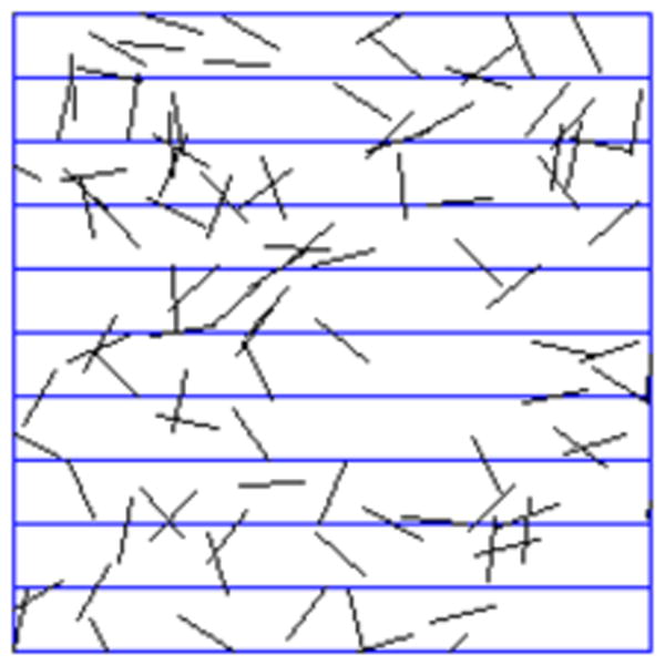
Buffon's Needle: after N tosses, the estimate for pi is (2N/X), where X is the number of times the needle intersects a line [2].

In the nineteenth and early twentieth centuries, simulation was increasingly used as an experimental means of confirming theory, analyzing data, or supplementing intuition in mathematical statistics. For example, E. L. De Forest (1834-1888), used a specially labeled card deck to develop and test a method of smoothing mortality tables; G. H. Darwin (1845-1912; Charles Darwin's son) used a spinner in an algorithm to smooth curves; F. Galton (1822-1911; C. Darwin's nephew) described a general simulation method using modified dice to generate a normal distribution; and W. S. Gosset (1876-1937) used labeled cards to help develop and test the t-test (under the penname A. Student), a means of testing the statistical significance of the difference between two sample means. [3]

These were seminal studies, but there is a significant difference between them and typical modern Monte Carlo simulations studying problems that are otherwise intractable, e.g. galaxy formation modeling. The early simulations dealt with previously understood deterministic problems. Modern simulation “inverts” the process, “treating deterministic problems by first finding a probabilistic analog” and “solving” the problem probabilistically [4].

This form of simulation was first developed and used systematically during the Manhattan Project, the American World War II effort to develop nuclear weapons. John von Neumann and Stanislaw Ulam suggested it to investigate properties of neutron travel through radiation shielding, and named the method after the Monte Carlo Casino in Monaco. They, along with others, used simulation for many other nuclear weapon problems and established most of the fundamental methods of Monte Carlo simulation.

Monte Carlo simulation is now a much-used scientific tool for problems that are analytically intractable and for which experimentation is too time-consuming, costly, or impractical. Researchers explore complex systems, examine quantities that are hidden in experiments, and easily repeat or modify experiments. Simulation also has disadvantages: it can require huge computing resources; it doesn't give exact solutions; results are only as good as the model and inputs used; and simulation software, like any software, is prone to bugs. Some feel it is overused, that people take it as a lazy way out, instead of analytical or experimental approaches. Analytic and experimental alternatives should be considered before committing to simulation.

The Monte Carlo Method

There is no single Monte Carlo method – any attempt to define one will inevitably leave out valid examples – but many simulations follow this pattern:

• - model a system as a (series of) probability density functions (PDFs);

• - repeatedly sample from the PDFs;

• - tally/compute the statistics of interest.

Defining The Model

In the case of Buffon's Needle, the model is based on a proof that shows the probability of the needle intersecting a line. To model the system one needs probability density functions for random positions in the lined space and random angles for the needle. It is a very simple simulation. Another paper in this volume, Monte Carlo Simulation Of Emission Tomography And Other Radiation-Based Medical Imaging Techniques, describes a more complicated model used to simulate emission tomography.

Key points to consider in defining a model are:

• - what are our desired outputs?

• - what will these outputs be used for?

• - how accurate/precise must the outputs be?

• - how exactly can/must we model?

• - how exactly can/must we define the inputs?

• - how do we model the underlying processes?

The outputs are key. What questions are we trying to answer? For instance, in a weather simulation we might want to predict high/low temperatures, likelihood/intensity of precipitation, and wind speed and direction for five days. The accuracy/precision needed will vary with use: predicting precipitation for picnic planning requires specifying which days rain is likely; for a farmer it may be more important to know how much rain will fall over the five days.

In addition to the desired outputs, the computing power available is often important in determining the inputs. For the most accurate weather simulation one would simulate all the interactions down to the subatomic level, but this is clearly far beyond both our computational capabilities and our ability to measure the inputs. Instead, weather simulations use fluid dynamics and thermodynamics, and the inputs are measured weather conditions at many locations around the globe. In the past several decades, weather simulations have gone from being useless for weather prediction (too slow, too imprecise) to being regularly used for forecasting as computers have gotten faster and inputs have become more exact (more weather measurement stations and increasing ability to measure conditions at multiple points vertically). Researchers see quite clearly the limits that input measurements place on their prediction abilities, as forecasts in areas in the middle of densely sampled regions (lots of weather stations, satellites, balloons, etc.) are more accurate than those near poorly sampled regions.

The final step in defining the model is determining how to process the inputs to generate the outputs. This is done deterministically in some simulations, for instance a weather simulation given the same inputs might always produce the same forecast. However, a Monte Carlo simulation always involves an element of randomness, often at many points in the model. In the weather simulation, one might include some randomness to account for the measurement error in the inputs; and the temperature, wind, and precipitation forecast for a given area might be time series for which each point is a random function of both the measurements and earlier time point forecasts in nearby areas. By running a Monte Carlo forecast multiple times, one could determine the variability of the forecast for the measured inputs.

Sampling From Probability Density Functions (PDFs)

At the base of a Monte Carlo simulation are the PDFs, functions that define the range of possibilities and the relative probability of those possibilities for a given step in the simulation. A PDF must be a non-negative real-valued function, and its integral over its range must be 1. For example, the PDF for the distance a photon will travel before interacting in an emission tomography simulation has a range of 0 to infinity; the probability for each distance is given by an exponential distribution, discussed below.

The uniform distribution with range from R to S, where R<S are real numbers, has a simple PDF: it gives equal probability to every number in its range

$$p(x)=\frac{1}{S-R},R\le x\le S$$ (1)

(the interval can also be open or half open as needed).

For sampling purposes we often use the cumulative distribution function (CDF), which is defined as an integral of the PDF, for the uniform distribution:

$$P(x)=\underset{R}{\overset{x}{\int }}p(x)=\frac{x-R}{S-R},R\le x\le S$$ (2)

The CDF tells us the probability that a number sampled randomly from the PDF will be ≤ x.

Random Number Generators (RNGs)

How can a computer generate a random number?

In general they don't. There are sources of truly random numbers, e.g. time between (detected) decays from a radioactive source (also see [5]). However, good ways have been found to generate pseudo-random numbers, with the advantage that sequences can be reproduced when testing or debugging.

A pseudo-random number generator, usually called an RNG (with the pseudo left out), is a deterministic computer algorithm that produces a series of numbers that shares many of the characteristics of truly random samples. There are many very good pseudo-RNGs available, and many tests have been developed to check how “random” they are (e.g. the Diehard tests [6] and TestU01 [7]). Most RNGs uniformly sample positive integer values between 0 and N. To sample the uniform distribution on [0,1], a sample, u, from the RNG is divided by N. Most RNGs allow N to be large enough that the double precision numbers between 0 and 1 are quite uniformly sampled using this method.

A very common RNG is the linear congruential generator (LCG). It is easy to understand and implement. Given the n^th sample, I_n, the next sample is

$$I_{n+1}=(a{I}_n+c)\text{mod}m$$ (3)

where a, c, and m must be carefully chosen for best performance. However, LCG is an older generator that even with the best choice of these constants doesn't do well on many tests in the Diehard suite or similar tests.

A more modern RNG, the Mersenne Twister, is rapidly becoming the generator of choice [8]. It is complicated but fast, passes most tests except for some that are for RNGs used in encryption, and has freely available source code [9].

Sampling From The Exponential Distribution Using The Inversion Method

The inversion method is one method to convert a uniform distribution sample to a sample from another distribution. It uses the uniform sample to “look up” a number on the other distribution's CDF. We'll demonstrate using the exponential distribution.

This distribution is very useful; it is, for instance, the distribution for the time between decays in a radioactive sample or the distance a photon travels before an interaction in a uniform medium.

The PDF (Fig. 2) of the exponential distribution is

FIGURE 2.

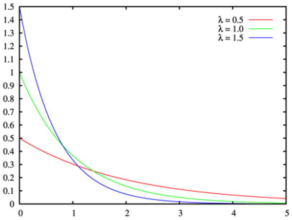
PDF For The Exponential Distribution [10].

$$f(x;\lambda )=\lambda e^{-\lambda x},x\ge 0$$ (4)

where λ adjusts the exponential decay. The CDF (Fig. 3) is

FIGURE 3.

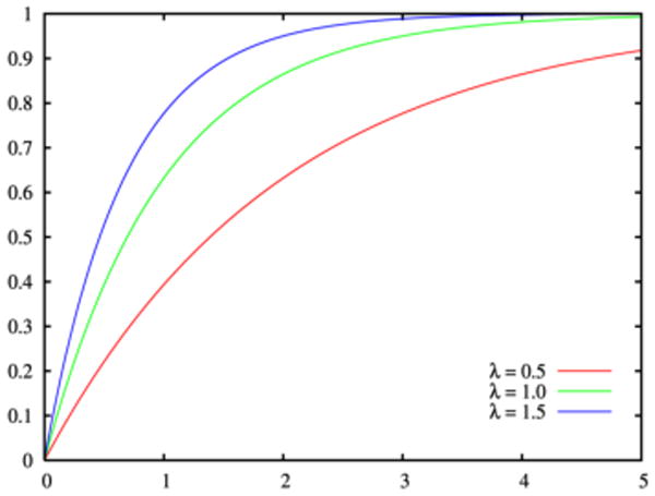
CDF For The Exponential Distribution [10].

$$F(x;\mu )=1-e^{-\lambda x},x\ge 0$$ (5)

To sample from the exponential distribution we use the following algorithm (Fig. 4):

FIGURE 4.

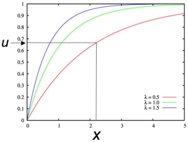
Sampling The Exponential Distribution. Given u from the uniform distribution, find x such that F(x)=u.

• - Sample u from the uniform distribution on [0,1);

• - Locate u on the y-axis of the CDF;

• - The x-value that corresponds to u is the random sample from the exponential distribution,

$$x=F^{-1}(u)\Rightarrow x=-\frac{\text{ln}(1-u)}{\lambda }$$ (6)

This method can be used to sample from any distribution that has an invertible CDF.

Sampling From Distributions: Other Methods

The acceptance-rejection method is often used when a CDF cannot be analytically inverted or the inversion is computationally burdensome. It is an exact sampling method, not an approximation. Its main disadvantage is that it requires two uniform random number samples for each sample in the target simulation. To sample from PDF f(x):

1. Choose PDF g(x) (with invertible CDF) and constant c such that c*g(x) ≥ f(x) for all x.

2. Generate a random number v from g(x) using the inversion method.

3. Generate a random number u from the uniform distribution on (0,1).

4. If c*u ≤ f(v)/g(v), v is the random sample

5. else reject v and go to 2.

In words, once a v is sampled from g(x), we accept or reject it in proportion to how much c*g(x) overestimates f(x) at v (Fig. 5). On average the method requires c iterations (steps 2-5) to produce a sample.

FIGURE 5.

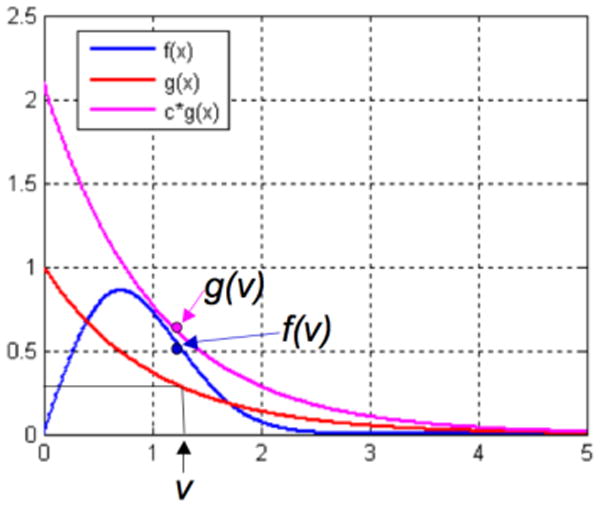
Acceptance-Rejection Method. Sample v from g(x) using method from the previous section, sample u from the uniform distribution, accept v if c*u ≤ f(v)/g(v) [11].

One can also sample from a distribution that approximates the desired distribution, for instance a piecewise-linear approximation. Such approximations often require a table lookup and an interpolation, and correctly implemented can be one of the fastest sampling methods. However, the approximation will add bias. If necessary, this bias can be removed by combining the approximation with the acceptance-rejection method, though the extra random number sample will negate any speed advantage in most cases.

Sampling From The Normal and Poisson Distributions

Two other PDFs that show up in many simulations are the normal and Poisson distributions.

The normal distribution (also known as a Gaussian or bell curve) is often used to approximate distributions when the true distribution is not known. This is not necessarily unjustified. An important statistical theorem, the central limit theorem, states that in the limit, a sum of independent random variables is approximately normally distributed. The PDF of the normal distribution (Fig. 6) is

FIGURE 6.

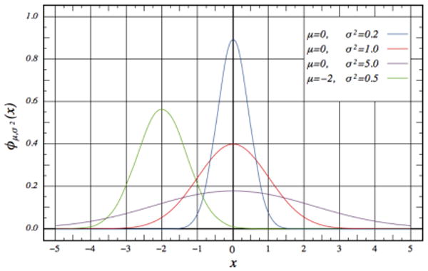
PDF For The Normal Distribution [12].

$$\phi (x;\mu ,{\sigma }^2)=\frac{1}{\sigma \sqrt{2\pi }}{e}^{-\frac{{(x-\mu )}^2}{2{\sigma }^2}}$$ (7)

where the parameters μ and σ give the mean and standard deviation respectively.

The CDF of the normal distribution is an invertible, but complicated function. As a result, the inversion method is slow and is not usually used for sampling. Fast acceptance-rejection algorithms have been developed, and are available in most numerical computing environments and libraries (e.g. [13]).

The Poisson distribution (Fig. 7) is a discrete distribution, with non-negative integer values. It gives the probability for how many events will occur in a fixed period if they occur randomly at known average rate, e.g., the number of decays from a radioactive sample in a second. The probability mass function (PMF, the discrete equivalent of the PDF) is

FIGURE 7.

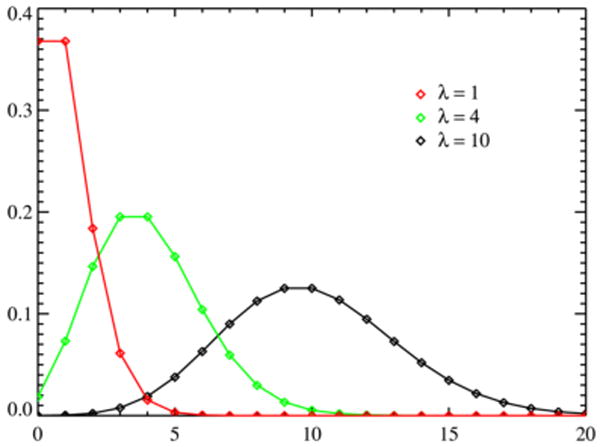
PMF For The Poisson Distribution [14]. The lines between the points are for clarity only; the PMF is a function of the non-negative integers only.

$$f(k;\lambda )=\frac{{\lambda }^k{e}^{-\lambda }}{k!}$$ (8)

where λ is both the mean rate and variance.

The Poisson distribution is related to the exponential distribution, which gives the time between events that occur at a fixed rate. The exponential distribution can be used to sample from the Poisson distribution: sample repeatedly from the exponential distribution until the sum of the samples is greater than the Poisson distribution's time period. The Poisson distribution sample is the number of exponential samples minus one. This is not a quick way to generate a sample, however. As with the normal distribution, we suggest that you use a library function.

Tallying Simulation Results

The final step of a simulation is to track the results. In general, Monte Carlo simulations repeat the same processes over and over, producing a series of events. The events are then recorded by their properties. For an example, see the paper Monte Carlo Simulation Of Emission Tomography And Other Radiation-Based Medical Imaging Techniques, also in this volume.

Summary

Monte Carlo simulation is a key tool for studying analytically intractable problems. Its history dates back to the eighteenth century, but it came into its modern form in the push to develop nuclear weapons during World War II.

Often a single ‘event’ in a simulation will require sampling from many different PDFs, some many times, and be tallied in many ways. Each sample will require one or more random numbers, and may require converting a uniform random number into a sample from another distribution using the inversion or acceptance-rejection methods.

References

- 1.Burger EB, Starbird MP. The Heart of Mathematics: an Invitation to Effective Thinking. New York: Springer-Verlag; 2005. p. 546. [Google Scholar]
- 2.Buffon's Needle. http://www.metablake.com/pi.swf.
- 3.Stigler SM. Statistics on the table: the history of statistical concepts and methods. Cambridge, Massachusetts: Harvard University Press; 2002. pp. 141–156. [Google Scholar]
- 4.Monte Carlo method. Wikipedia. http://en.wikipedia.org/wiki/Monte_Carlo_method.
- 5.Random.org. http://www.random.org.
- 6.Diehard tests. Wikipedia. http://en.wikipedia.org/wiki/Diehard_tests.
- 7.L'Ecuyer P, Simard R. TestU01: A C Library for Empirical Testing of Random Number Generators. ACM Trans Mathem Softw. 2007;33(4) Article Number: 22. [Google Scholar]
- 8.Mersenne Twister. Wikipedia. http://en.wikipedia.org/wiki/Monte_Carlo_method.
- 9.Mersenne Twister: A Random Number Generator. http://www.math.sci.hiroshima-u.ac.jp/∼m-mat/MT/emt.html.
- 10.Exponential distribution. Wikipedia. http://en.wikipedia.org/wiki/Exponential_distribution.
- 11.Acceptance-Rejection Methods. Statistics Toolbox – Documentation. http://www.mathworks.com/access/helpdesk/help/toolbox/stats/bqttfc1.html.
- 12.Normal distribution. Wikipedia. http://en.wikipedia.org/wiki/Normal_distribution.
- 13.Press WH, et al. Numerical Recipes In C: The Art Of Scientific Computing. 2nd. Cambridge: Cambridge University Press; 1992. pp. 288–290. [Google Scholar]
- 14.Poisson distribution. Wikipedia. http://en.wikipedia.org/wiki/Poisson_distribution.