PeakSeq: Systematic Scoring of ChIP-Seq Experiments Relative to Controls

Abstract

Chromatin immunoprecipitation followed by tag sequencing (ChIP-Seq) using high-throughput next-generation instrumentation is replacing ChIP-chip for mapping of sites of transcription-factor binding and chromatin modification. To develop a scoring approach for this new technique, we produce two deeply sequenced datasets for human RNA polymerase II and STAT1 with matching input-DNA controls. In these, we observe that signal peaks corresponding to sites of potential binding are strongly correlated with peaks in the control, likely revealing features of open chromatin. Based on these observations, we develop a two-pass approach for scoring ChIP-Seq relative to controls. The first pass identifies putative binding sites and compensates for genomic variation in the mappability of sequences. The second pass filters sites not significantly enriched compared to the normalized control, computing precise enrichments and significances. Using our scoring we investigate optimal experimental design – i.e. depth of sequencing and value of replicas (showing marginal information gain beyond two).

With the advent of new high-throughput sequencing technologies (Helicos HeliScope, Illumina Genome Analyzer, ABI SOLiD, Roche 454), most genome scale assays that previously could only be done cost-effectively using genomic tiling microarrays can now be performed using DNA sequencing. One of the most common uses of tiling microarrays is for performing ChIP-chip^1-3. In ChIP-chip, DNA associated with a protein of interest is immunoprecipitated using an antibody specific to that protein (chromatin immunoprecipitation or ChIP) and the resulting DNA is labeled and hybridized to a genomic tiling microarray. Early adaptations of ChIP sequencing (e.g. STAGE⁴, ChIP-PET^5,6) used Sanger-based sequencing, which generally provided limited tags and/or was expensive. The new analog of this experiment is called ChIP-Seq^7,8, in which millions of short tags are sequenced from the immunoprecipitated DNA fragments. More than 100 ChIP-chip experiments were performed during the pilot phase of the ENCODE project⁹; however, in the scale up to the whole human genome almost all ChIP experiments are being done utilizing ChIP-Seq. Moreover, ChIP-Seq is being used extensively for the modENCODE project.

Short tag sequencing platforms yield sequence reads of sufficient length to uniquely map most tags and their associated DNA fragments to the genome of interest. The Illumina Genome Analyzer platform, formerly Solexa, was the first truly high-throughput sequencing technology to gain widespread usage for ChIP-Seq. Each lane of data typically generates several million ~30 nt sequence tags. Mapping these tags against the genome, we can identify regions that are overrepresented in the number of mapped tags or fragments, which might correspond to genomic locations of transcription factor binding. However, there are a number of issues that make scoring more complicated. In this paper we develop a general methodology for analyzing ChIP-Seq data using two deeply (as compared to previously published) sequenced ChIP-Seq datasets: human RNA polymerase II (Pol II) and STAT1. Pol II, a component of the general transcriptional machinery and STAT1, a representative sequence-specific transcription factor, both bind primarily to punctate regions of DNA in what is typically called point-source binding. To help determine experimental design we further analyze target identification as a function of sequencing depth (i.e. saturation) and the number biological replicas required.

RESULTS

Characteristics of ChIP-Seq Data

ChIP-Seq datasets were generated for both Pol II in unstimulated HeLa S3 cells (an immortalized cervical cancer derived cell line) as well as STAT1 in interferon-γ stimulated HeLa S3 cells (STAT1 is induced when a cell is stimulated by interferon-γ). Matching control input DNA-Seq datasets were obtained for both stimulated and unstimulated cells (see Methods). Although we chose to use input DNA as the control, we could have used a ChIP-Seq with a different antibody (i.e. IgG) or a ChIP-Seq sample under a different cellular condition (i.e. unstimulated STAT1 ChIP).

In the first and third tracks of Figure 1a we see the signal maps for both HeLa S3 Pol II and STAT1 for a region on chromosome 22. The vertical axis is the count of overlapping mapped DNA fragments at each nucleotide position. Peaks (large numbers of overlapping mapped fragments) in this track correspond to regions of DNA where either Pol II or STAT1 has potentially bound in the HeLa S3 cell-line being studied. Ideally the background to this experimentally generated signal map would be a randomly generated map with the same number of mapped fragments (i.e. a uniform background distribution). If this were the case, peaks in the random background would follow Poisson statistics and could be computed either theoretically or by simulation. A peak threshold could then be set based on a false discovery rate determined by the number of peaks from the background distribution compared to the actual data⁷.

Figure 1. ChIP-Seq Characteristics.

1a) The first and third signal tracks are plots of mapped fragment density for Pol II (in blue) and STAT1 (in red), respectively. The second and fourth tracks correspond to the input DNA tracks for unstimulated (in blue) and interferon-γ stimulated HeLa S3 cells (in red). The vertical axis for the first four tracks is the count of the number of overlapping DNA fragments at each nucleotide position (peaks in the top track indicated with a star have been truncated). The fifth track shows the fraction of uniquely mappable bases plotted in 1 kb bins (in green). We observe that many of the peaks in the Pol II and STAT1 tracks match corresponding peaks in the input DNA controls, only some of which are enriched in their height relative to the control. 1b) Here we see the signal for Pol II (solid blue line), STAT1 (solid red line) ChIP-Seq and corresponding unstimulated (dashed blue line) and interferon-γ stimulated (dashed red line) input DNA controls aggregated over regions proximal to all human CCDS transcription start sites (± 2.5 Kb) plotted in 100 bp bins. We observe significant enrichment for both transcription factors as well as the input DNA controls over TSSs. The aggregated signal for the fraction of mappable bases is also plotted (green line) and we also observe a smaller but significant enhancement over TSSs (see insert where the vertical scale is from 0.95 to 1.15), though not as pronounced as the sequencing results.

Unfortunately, the background distribution for a ChIP-Seq experiment is not this simple¹⁰. There are multiple effects that contribute to the signal map from a ChIP-Seq experiment. Firstly, since sequence tags from certain genomic locations are not unique to the genome, sequenced reads from these regions would not be included, as they do not align uniquely to the genome. Thus the distribution of uniquely mappable bases in the genome is not uniform (see the fifth track of Fig. 1a).

Secondly, genomic DNA isolated from cells is in the form of chromatin: DNA tightly wound around nucleosomes. The structure of chromatin might bias the amount of DNA that is experimentally observable from different regions of the genome. In the second and fourth tracks of Figure 1a we observe that there are also peaks in the signal maps for unstimulated and interferon-γ stimulated HeLa S3 input DNA in the vicinity of promoters of known genes, which may correspond to regions of open chromatin¹¹. This can also be seen in Figure 1b, in which the signal maps have been aggregated proximal to transcription start sites (TSSs), i.e. within ±2.5 Kb, for all annotated CCDS genes (a consensus set of gene annotation¹², uniformly agreed upon by Ensembl, NCBI and UCSC) in the human genome.

Thus the signal map of aligned fragments for a given transcription factor is actually the “convolution” of a number of effects: the density of mappable bases in a region, the underlying chromatin structure and the actual signal from transcription factor binding. Therefore some fraction of the peaks in the ChIP-Seq signal map for a transcription factor might be due to the nature of the chromatin structure in those regions, i.e. regions of open chromatin. In order to ascertain that the signal for any region is enriched due to the presence of transcription factor binding it is necessary to compare the signal against that from a control such as a matching sequenced input DNA experiment.

Mappability Map of a Genome Sequence

A significant advantage of using tag-based sequencing instead of tiling microarrays for unbiased genomic experiments is that it is possible to cover a significantly greater fraction of the genome. This is especially true for the more complex mammalian genomes that are almost equally comprised of repetitive and non-repetitive sequence. In Table 1 we compute the fraction of the genomes of four well-studied organisms (worm, fruit fly, mouse and human) that are assayable using either tiling arrays or tag sequencing based technologies. For human we find that even though only 47.5% of the genome is non-repetitive, 79.6% of the genome is uniquely mappable using 30 nt sequence tags. Even for more compact genomes such as the worm, which has significantly less repetitive sequence than human, a significant gain in coverage is achieved by using a tag-sequencing based approach (86.8% to 93.0% coverage with 30 nt tags). As next generation sequencing technologies improve longer sequence reads become possible. We find that the fraction of the human genome that is uniquely mappable increases from 79.6% to 89.3% as the length of the sequenced tag is increased from 30 to 70 nt.

Table 1. Genome Mappability Fraction.

For four common model organisms; worm, fruit fly, mouse and human we have determined the fraction of each genome sequence that is non-repetitive as well as the fraction that is mappable using 30 nt sequence tags. The genome coverage achievable from genomic tiling arrays corresponds to the non-repetitive fraction of a genome while the mappable coverage is what is achievable by tag-based sequencing approaches. We also determined that as the length of the sequence tags is increased beyond 30 the number of nucleotides in the genomes that are uniquely mappable is 2,452 Mb (79.6%) for 30nt reads, 2,586 Mb (84.0%) for 40 nt, 2,669 Mb (86.7%) for 50 nt, 2,720 Mb (88.3%) for 60 nt and 2,750 Mb (89.3%) for 70 nt.

Organism	Genome Size (Mb)	Non-Repetitive Sequence		Mappable Sequence
		Size (Mb)	Percentage	Size (Mb)	Percentage
C.elegans	100.28	87.01	86.8%	93.26	93.0%
D.melanogaster	168.74	117.45	69.6%	121.40	71.9%
M.musculus	2,654.91	1,438.61	54.2%	2,150.57	81.0%
H.sapiens	3,080.44	1,462.69	47.5%	2,451.96	79.6%

We have developed code for efficiently indexing an entire genome and then determining at each nucleotide position the number of locations at which a sequence tag of length k appears in the entire genome (see Supplementary Material). Analysis of the idealized achievable genome coverage from short tag sequencing has previously been investigated¹³. The output from the code is a binary file for each chromosome containing a table that maps from a position on the chromosome to the number of occurrences in the whole genome of the k-mer starting at that position. The mappability map that we construct only accounts for sequence tags that are located multiple places in the genome and that are identical, i.e. no mismatches are allowed. We have also investigated the effect of allowing for mismatches in the mappability map (see Supplementary Material).

As shown in the fifth track of Figure 1a, we have determined the fraction of uniquely mappable nucleotide positions using genomic windows of 1 Kb. We also have generated a profile of the fraction of alignable bases aggregated across all CCDS TSSs in the human genome and note a small but statistically significant enrichment in the fraction of alignable bases proximal to known TSSs (inset in Fig. 1b). The enhancement in mappable bases proximal to TSSs of genes is likely due to the increased complexity of DNA sequences in promoter regions.

Input DNA

In order to determine that a “peak” in the signal map of DNA fragments actually corresponds to a site of transcription factor binding, it is necessary to show that the signal obtained is enriched compared to a matched control sample such as input DNA isolated from the same cell line under the same cellular conditions that the ChIP experiment is performed, i.e. HeLa S3 cells stimulated by interferon-γ for the case of STAT1. Observing the signal maps (tracks 2 and 4 of Fig. 1a) for input DNA we first observe that the distribution is not the “flat” distribution one would expect from a random Poisson process. We observe more significant “peaks” than would be expected from a random distribution. By analyzing the number of sites as a function of peak height it has been shown that this distribution cannot arise from a uniform background distribution¹⁰. There is a significant correlation between the locations of peaks present in the input DNA signal map and the matching ChIP-Seq results (Supplementary Material).

Using the signal maps of DNA fragments we created profiles of the aggregated signal maps proximal to the TSSs of well-annotated CCDS genes (see Figure 2). In addition we created profiles for both Pol II and STAT1. Although the aggregated profiles for HeLa S3 input DNA are not as pronounced as the aggregated signals from Pol II and STAT1, the input DNA under both conditions exhibits distinctive enrichments of signal proximal to TSSs. This again demonstrates that the peaks in the input DNA signal do not arise from a random background distribution. We also note that the aggregated signals yield a higher definition profile with finer resolution as compared with the aggregated ENCODE ChIP-chip profiles⁹.

Figure 2. PeakSeq Scoring Schematic.

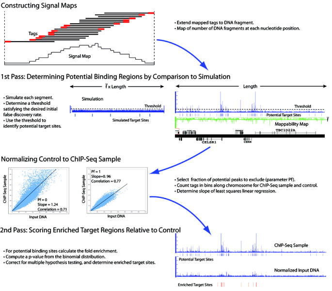
We present a schematic of the scoring procedure. 1) Mapped reads are extended to have the average DNA fragment length (reads on either strand are extended in the 3’ direction relative to that strand) and then accumulated to form a fragment density signal map. 2) In the first pass of the PeakSeq scoring procedure potential binding sites are determined. The threshold is determined by comparison of putative peaks with a simulated segment with the same number of mapped reads. The length of the simulated segment is scaled by the fraction of uniquely mappable starting bases. 3) After selecting the fraction of potential targets sites that should be excluded from the normalization, P_f, a scaling factor is determined by linear regression of the ChIP-Seq sample against the input DNA control in 10 Kb bins. Bins that overlap the potential targets regions selected for exclusion are not used for regression. The fitted slopes as well as the Pearson correlations are displayed for P_f set to either 0 or 1. 4) Enrichment and significance are computed for putative binding regions.

The aggregated profiles for the input DNA samples proximal to TSSs are substantially more enriched than the relatively minor enrichment coming from the profiles of mappable bases (insert in Fig. 1b). This shows that although the mappability map is a component of the input DNA signal, it only explains a relatively small portion of the enrichment proximal to TSSs. However, if one views the genome at a more coarse-grained level (averaged over 10 Kb windows) then we observe that when we scale the coarser-grained input DNA signals by the fraction of mappable bases, the signal is more uniform than the signal before scaling. This shows that the fraction of mappable bases plays a substantial role in modulating the signal we observe.

PeakSeq: Scoring ChIP-Seq Data

Based on these observations and our experience with scoring of ChIP-chip experiments¹⁴, we develop an approach, called PeakSeq, for scoring the results of ChIP-Seq experiments by compensating for the mappability map and comparing against a normalized matching control dataset. For computational efficiency we adopt a two-pass approach for scoring ChIP-Seq data relative to a control dataset. A schematic of the procedure is presented in Figure 2 (see Methods for further details of each step).

Construction of Signal Maps

In order to accommodate the large datasets that are typically generated, we process all ChIP-Seq data on a chromosome-by-chromosome basis. Using only uniquely mapping reads we generate signal maps along each chromosome for the ChIP-Seq dataset as well as the matching control dataset. Signal maps are generated by extending each mapped tag in the 3’ direction (as sequences are read from the 5’ end), to the average length of the DNA fragments in the sequenced DNA library (~200 bp). The signal map is then the integer count of the number of overlapping DNA fragments at each nucleotide position (see first panel of Fig. 2).

First Pass: Identification of Potential Target Sites

Motivated by the scoring procedure developed in Robertson et al.⁷, in the first pass of our approach we focus on the ChIP-Seq dataset and identify regions or peaks in the ChIP-Seq fragment density map that are significantly enriched compared to a simulated simple null background model. In order to capture some level of genomic variability (such as copy number variation^15,16) this analysis is done on a segment-by-segment basis along each chromosome; segments are by default 1 Mb (second panel of Fig. 2). Within each segment we use the mappability map to correct for the variation in mappability between segments. The candidate regions that are identified as potential DNA binding sites are not necessarily locations of transcription factor binding, as they may also be present in the input DNA control. The first pass of the PeakSeq procedure acts as a pre-filter in which candidate regions are selected for comparison against the input DNA control.

Normalization of Control to ChIP-Seq Sample

In order to compare the number of mapped tags to a potential binding site from the ChIP-Seq sample compared to the control we need to normalize the control against the sample. We normalize the background of the sample to the control by linear regression of the counts of tags from the control against the sample for windows (~10 Kb) along each chromosome. The slope of the linear regression α is used to scale tag counts from the control in the comparison with the ChIP-Seq sample. Since windows that contain enriched peaks will cause the slope to be larger (conservatively over-estimating the tag counts from the control) we introduce a parameter, P_f, the fraction of potential target regions that we exclude from the normalization procedure (windows that overlap excluded target regions are not used in the linear regression). In the third panel of Figure 2 we show the effect of the normalization procedure for two settings of this parameter (P_f = 0 and P_f = 1).

Second Pass: Scoring Target Sites Relative to Control

In the second pass of the procedure (last panel of Fig. 2), the ChIP-Seq signals for putative binding sites are then compared against the normalized input DNA control. Only regions that are enriched in the counts of the number of mapped sequence tags in the ChIP-Seq sample relative to the input DNA control are called binding sites. This comparison is analogous to the way enrichment is determined when validating ChIP “hits” using qPCR. We compute the statistical significance using the binomial distribution. We also correct for multiple hypothesis testing by applying a Benjamini-Hochberg correction¹⁷. We report a ranked target list sorted by q-value that also lists fold enrichment values for each binding site. Comparison of potential target binding sites in the ChIP-Seq sample against the input DNA control accounts for the non-uniform background of a ChIP–Seq experiment¹⁰.

Application of PeakSeq to Pol II and STAT1 ChIP-Seq Data

Scoring Pol II and STAT1 ChIP-Seq Data using PeakSeq

We apply PeakSeq procedure to the Pol II and STAT1 ChIP-Seq datasets (we conservatively set P_f = 0 in the following analysis). We initially identify 73,562 and 123,321 potential binding sites for Pol II and STAT1, respectively. These represent the potential targets that are found to be significant in the Pol II and STAT1 signal density maps compared to a simulated null random background. After comparison with the normalized input DNA controls (unstimulated and interferon-γ stimulated HeLa S3 cells) we find that only 24,739 and 36,998 of these target regions are significantly enriched for Pol II and STAT1, respectively (using a false discovery rate threshold of less than 0.05). In Supplementary Table 2 we demonstrate how the number of target binding sites varies for a range of different false discovery rate thresholds for each target list.

Scaling of Identified Targets

In Figure 3 we divide the putative targets identified for Pol II (left panel) and STAT1 (right panel) into targets that are enriched (blue) and those that are not significantly enriched (red). Plotted on a log-log scale the horizontal axis is the count of the number of sequence tags overlapping a putative binding region. We observe that both the enriched and unenriched (potential binding sites that are not enriched compared to the input DNA control) distributions display an approximate power-law behavior. These plots are consistent with those generated for models of different background distributions¹⁰. However, the slope of the distribution of regions that are not enriched is steeper than that of the enriched distribution.

Figure 3. ChIP-Seq Target List Scaling.

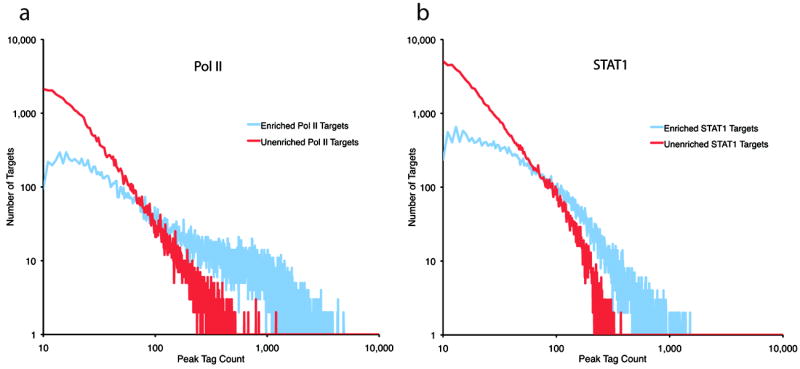
On a log-log plot we show the distribution of target regions that are enriched (blue) relative to input DNA and those that are not (red). The horizontal axis is the count of the sequence tags that are within a target peak while the vertical axis the number of target regions with that count. The left and right panel shows the results for Pol II and STAT1, respectively.

Comparison of PeakSeq Results with Published ChIP-chip and ChIP-Seq Data

We also compared the results obtained for Pol II and STAT1 ChIP-Seq against matching pilot-phase ENCODE ChIP-chip datasets⁹. We find that 1,499 Pol II binding sites of average size 275 bp and 1,164 STAT1 binding sites of average size 128 bp are present in the one percent of the genome studied. Correspondingly, for ChIP-chip 1,000 Pol II sites of average size 1,300 bp and 395 STAT1 sites of average size 507 bp were identified (ChIP-chip experiments were performed using Nimblegen ENCODE tiling microarrays). We find that 321 (32.1%) of the ENCODE Pol II ChIP-chip sites are common to the matching ChIP-Seq target lists. For the case of STAT1 many of the ChIP-chip target sites were independently tested for validation by qPCR⁶. We find that 106 of the 128 (83%) of the validated targets are common to the STAT1 ChIP-Seq target list. By comparison only 26 of the 282 (9%) regions were not validated by qPCR are present on the ChIP-Seq target list. In both cases, ChIP-Seq was able to detect more binding sites (substantially more for STAT1) with higher resolution (i.e. more localized binding sites). A representative example of the cytokine receptor locus on chromosome 21 comparing ChIP-Seq and ChIP-chip for Pol II and STAT1 is displayed in Figure 4.

Figure 4. ChIP-Seq vs ChIP-chip.

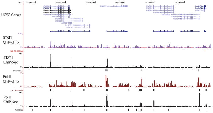
In this figure we show the signal tracks and target binding sites for Pol II and STAT1 for both ChIP-chip and ChIP-Seq. The ChIP-chip data was generated as part of the pilot-phase of the ENCODE project for one percent of the human genome. The region displayed is the cytokine receptor locus on chromosome 21. We observe that the ChIP-Seq signal has better signal to noise and is higher resolution than the corresponding ChIP-chip data. Data was obtained from the UCSC Genome Browser¹².

We find that 21,750 of the 36,998 STAT1 ChIP-Seq target sites (58.7%) are in common with the ChIP-Seq results from Robertson et al.⁷ (see Supplementary Material for details). We also ran the ChIPSeqMini⁸ software on the Pol II ChIP-Seq data produced in this paper and 9,467 target binding sites were identified with a median size of 1,939 bp. By comparison PeakSeq identified 24,739 sites with a median size of 841 bp. Using the same data and the same hardware PeakSeq ran in under 8 minutes while ChIPSeqMini required 459 minutes to run. All the regions identified by ChIPSeqMini overlap regions called by PeakSeq, which is consistent with ChIPSeqMini using a more restrictive threshold in calling peaks, even though the regions identified are broader. The most significant peaks identified in the initial peak-calling pass of PeakSeq tend to all be significantly enriched compared to the input DNA control.

Implications for the Optimal Design of ChIP-Seq Experiments

Depth of Sequencing

In order to investigate the depth of sequencing required to saturate the number of identifiable target binding sites we performed the following analysis. For both the Pol II and STAT1 ChIP-Seq datasets we shuffle the mapped sequence reads in order to remove any biases due to the variation between biological replicas or different flowcell lanes. The sequences for each of the input DNA controls were similarly shuffled.

Initially, for each transcription factor one million reads were selected from both the randomly ordered sample and control sequences. These datasets were scored, identifying both potential targets for binding as well as the subset of these that are enriched compared to the control. For increasing numbers of reads we scored putative and enriched target sites (larger sets of reads are inclusive of smaller sets).

In Figure 5c we plot the number of identified putative targets (dashed lines) and enriched targets (solid lines) for both Pol II (blue) and STAT1 (red). We observe that the number of Pol II targets is saturating as a function of sequencing depth. The number of targets for Pol II appears to be approaching an asymptotic value of ~25,000 target regions. Curiously, the number of targets identified for STAT1 initially climbs much slower than Pol II; however, the number of targets continues to rise and is only starting to show signs of plateauing once 22.5 million reads have been analyzed. This is consistent with the larger proportion of Pol II targets that show higher levels of enrichment as compared to STAT1. We note that for both Pol II and STAT1 the number of putative target regions continues to increase significantly as a function of sequencing depth. This analysis implies that the set of identified sites is approaching the total number of target sites (or that the total number of sites is saturating). However, formally this is not a proof of saturation as in principle there could be another regime after some critical number of sequence reads where it is possible to identify a novel class of enriched regions (i.e. broad-binding domains).

Figure 5. Depth of Sequencing and Value of Replicas.

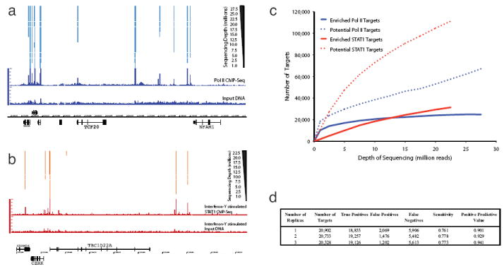
5a) Fragment density signal tracks are plotted for Pol II and the input DNA control as well as the target regions that are identified (significantly enriched) as a function of the number of mapped sequence reads. The same numbers of sequence reads are used for both sample and control. More prominent peaks are identified with fewer reads, while weaker peaks require greater depth. 5b) Similar plot with STAT1 and matching interferon-γ stimulated HeLa input DNA control. 5c) Here we plot as a function of the number of mapped sequence reads the number of putative Pol II (blue line) and STAT1 (red line) targets identified and the fraction for each of these that are enriched relative to input DNA. We see that while the number of putative targets continues to climbs for both Pol II and STAT1 the number of enriched targets begins to plateau. The number of Pol II targets appears to be saturating faster than STAT1. 5d) We summarize the results of analyzing 9 million mapped Pol II ChIP-Seq sequence reads using 1, 2 or 3 biological replicas. We calculate sensitivity and positive predictive values using the targets identified with all the available sequence reads (~29 million uniquely mapped reads) as gold standard positives and the remainder as negatives. Only a marginal gain in positive predictive value at the cost of sensitivity is gained by using 3 biological replicas instead of 2 biological replicas.

In Figure 5a and 5b we display the target binding sites that are significantly enriched as a function of the number of mapped sequence reads. We observe that the most prominent peaks are identified with only one million sequences: however, smaller peaks are only called when more sequences are included.

Number of Biological Replicas

Biological replicas in high-throughput genomic experiments are performed to achieve two disparate objectives: to ensure that experiments are reproducible and to quantify the biological variation between samples in an experiment. As part of the pilot phase of the ENCODE project⁹ it was decided that three biological replicas were necessary for ChIP-chip experiments in order to ensure reproducibility. What is the optimal number of biological replicas necessary for a ChIP-Seq experiment?

In order to quantify the gain in the number of enriched target binding sites identified by adding additional biological replicas, we performed the following analysis using the ~29 million uniquely mapped sequence reads for Pol II ChIP-Seq that were generated using three independent biological preparations. We conducted the analysis where, using the same total number of mapped reads, we separately analyzed the results using sequences coming from increasing numbers of replicas. Care needs to be taken to ensure appropriate randomization of reads and permutations of replicas and flowcells/lanes to avoid biases (see Methods).

Using the target list identified from all the available Pol II ChIP-Seq data as a gold standard set of positives (and all other regions as negatives) we compared the target lists identified using 9 million reads from only one biological replica, or from two replicas or from all three replicas and computed the sensitivity and positive predictive value for each target list. We then calculated the average sensitivity and positive predictive value for one replica (averaged over all three), two replicas (averaged over all three pairs) and three replicas (results summarized in Fig. 5d).

We observe some gain in sensitivity and positive predictive value when the number of biological replicas is increased from one to two. However, there is no further increase in sensitivity when using three replicas and the positive predictive value only increases marginally. In a ChIP-Seq experiment it is necessary to perform at least two replicas in order to be able to ensure that experimental results are reproducible (in order to identify a failed experiment); however, it is not clear that there is a significant information gain beyond two independent replicas. Consequently the ENCODE consortium currently requires greater than 90% agreement between target lists from biological replicas.

DISCUSSION

In this paper we have demonstrated that there are two main observed effects that modulate the ChIP-Seq signal profile: the genomic variation in the fraction of mappable sequence tags and differences in chromatin accessibility as evidenced in input DNA-Seq control experiments. These two effects can be contrasted with the two main biases that affect tiling array ChIP-chip experiments: probe-to-probe hybridization differences and cross-hybridization¹⁸. In reality we use the same input DNA control in ChIP-chip experiments and the same chromatin features should be present when observing the signal for the single channel input DNA control. This is typically not apparent as the other two effects that are more pronounced obscure this signal. The effect of the input DNA is the same for ChIP-chip and is normally scaled out when the ChIP-chip signal is scored in the typical two-channel fashion.

One might think that ChIP-Seq experiments are immune to the probe-specific effects and cross-hybridization that both occur for ChIP-chip; these two effects can be contrasted against the genomic variation in mappable sequence tags, which plays a similar role in the analysis of ChIP-Seq datasets. One fundamental difference between ChIP-chip and ChIP-Seq is that the signal for ChIP-chip is a continuous-valued fluorescent intensity for each oligonucleotide probe, whereas the signal for ChIP-Seq is a discrete integer-valued count of the number of mapped tags in a genomic region. This affects the analysis and the type of statistics used. Motivated by the way ChIP-chip experimental data are analyzed we have developed an approach for scoring ChIP-Seq data accounting for variation in mappability and input DNA controls. Initial analyses of ChIP-Seq^7,8 experiments did not account for these effects and target regions were not scored relative to an appropriate control experiment.

Although we have initially implemented our methodology for use with tag sequence data from the Illumina Genome Analyzer platform, it should be relatively straightforward to adapt it for use with other high-throughput sequencing platforms. We have developed the PeakSeq approach to identify peak regions in ChIP-Seq datasets that correspond to sites of transcription factor binding. Although we have used input DNA as a control in this paper, other controls can be used (e.g. unstimulated STAT1 ChIP or IgG). We have also shown that separate input DNA control samples are needed for different cellular conditions even for the same cell-line (see Supplementary Material). Even though this approach has been developed and calibrated to identify sites for more punctate point-source binding of transcription factors or proteins to DNA, it can also be used to identify broader regions of binding (such as histone modifications) that show significant enrichment relative to control. However, a more detailed procedure will be necessary for identifying extended regions of binding. A significant feature of our analysis methodology is that statistical quantities such as false discovery rates and p-values are based on the number of target regions identified rather than the number of enriched nucleotides. In our approach we treat sequence tags mapping to the forward and reverse strands equally (tags are sequenced from the 5’ ends of DNA fragments). One could compare the relative orientation of these reads in each target region compared to what would occur by chance.

For certain transcription factors ChIP-Seq surpasses ChIP-chip for identifying sites of transcription factor binding⁷. By analyzing the signal data between ChIP-Seq and ChIP-chip data it is evident that ChIP-Seq data gives finer resolution and greater signal-to-noise (see Figure 4). ChIP-Seq also achieves a significantly greater coverage of the genome of interest as compared with ChIP-chip using tiling arrays, especially for the larger mammalian genomes. The fold enrichment determined for ChIP-Seq typically shows a significantly greater range than does ChIP-chip; this is understandable as effects such as cross-hybridization tend to reduce the fold enrichment from a tiling array approach. While ChIP-Seq appears to significantly outperform ChIP-chip it is not clear that this will be the case for all transcription factors and chromatin modifications, especially those that bind to broader genomic regions where it might be necessary to sequence extremely deeply in order to achieve better results than from tiling arrays.

METHODS

Generation of Illumina Tag Sequencing Data

For this paper we generated two deeply sequenced ChIP-Seq datasets for antibodies against both human RNA polymerase II and STAT1 performed in the HeLa S3 cell line. For Pol II using the results from 24 lanes of Illumina sequencing data we obtained more than 29 million mapped reads for the Pol II ChIP-Seq as well as a matching 29 million reads for a control sample of HeLa S3 Input DNA. STAT1 ChIP was performed in HeLa S3 cells that had been stimulated using interferon-γ, producing 26 million mapped reads for IFN-γ stimulated STAT1 ChIP DNA. We obtained 24 million mapped reads for a matching control of IFN-γ stimulated HeLa S3 input DNA. See Supplementary Material for further details of experimental protocols. A complete breakdown of the ChIP-Seq reads generated is summarized in Supplementary Table 1. Raw and aligned sequence reads for all datasets have been deposited at GEO with accessions numbers: GSE12781 (Pol II) and GSE12782 (STAT1).

Illumina Data Analysis Pipeline

Raw image files from the Illumina Genome Analyzer machine are transferred to the Yale biomedical high-performance computing cluster. Data is processed following the recommended Illumina pipeline. Raw images are first processed using the Firecrest software package. Base-called sequences with confidence metrics are obtained using the Bustard software. Gerald is the last part of the pipeline. It uses the program ELAND to align the short sequence reads against the genome of interest allowing for up to 2 possible mismatches. By default ELAND only gives the locations for reads that align uniquely to the target sequence; however, with modified parameters ELAND can report the locations for reads that map to multiple locations. For the human ChIP-Seq and control datasets we aligned the sequence reads to the latest build of the human genome (hg18/NCBIv36) obtained from the UCSC Genome Browser¹². We excluded the random unassembled contigs.

Alignment of Tag Sequences

Following a typical analysis pipeline, flowcell images are analyzed, yielding base called sequences with confidence scores, which are then aligned against the appropriate genome. The standard Illumina pipeline utilizes the program Eland for aligning sequence tags, although a number of other applications have been developed for the same purpose, e.g. Maq¹⁹, Rmap (unpublished), SOAP²⁰. When aligning sequence reads against the genome, reads aligning to multiple locations are typically excluded, as they are ambiguous (see Supplementary Table 1 to see the proportion of sequence reads generated that map to multiple locations in the human genome). However, such exclusion results in portions of the genome, including highly repetitive sequences or recent segmental duplications, that are not alignable and thus not assayable.

Although the algorithm we have developed by default only utilizes sequence tags that map uniquely, it would be a relatively straightforward modification to utilize tags that map to multiple locations by capping the number of locations to which a tag is allowed to map and by weighting tags by a factor dependant on the number of locations to which it maps or randomly selecting one of the locations. Many of the mapping algorithms including Eland and Maq have options allowing for the aligning of sequence reads to multiple locations in the genome. The effect of including sequence reads that map to multiple locations in the scoring is also discussed in these Methods.

PeakSeq: First Pass Identification of Potential Target Sites

Once fragment density maps have been created for both the sample and control datasets, we initially focus on the sample density map. Each chromosome is subdivided into segments of length L_segment (typically 1 Mb) for analysis. Depending upon the genome being analyzed one might select a different size for these segments, e.g. smaller segments for more compact genomes. For each segment the number of fragments that align to that segment are counted, N_reads. In addition by using the mappability map for the genome of interest, we can precompute the fraction of uniquely alignable bases in that segment, f (see methods for further details). Using these two parameters, N_reads and f we can perform a computational simulation by randomly generating N_reads aligned DNA fragments in a scaled segment of length f×L_segment (see second panel of Figure 2 and below for details of the simulation). In order to perform an accurate simulation this is done multiple times and the results of these simulations are averaged.

Using a height threshold we can determine all the contiguous regions that are above this threshold in the sample fragment density map. Regions above threshold that are separated by genomic distances less than the average fragment length (~200 bp) are merged. This is similar to the maxgap/minrun approach that is commonly used for analyzing ChIP-chip tiling array data^14,21. For the same threshold we can determine the number of merged regions above the threshold in the simulation. For each threshold the fraction of false positives is calculated from the ratio of the estimated number of false positives above threshold from the simulation divided by the number of regions above threshold for the ChIP-Seq sample. By tuning the threshold used we can set an initial first pass false discovery rate (the false discovery rate for the final list of target binding sites will be determined after comparison with the control sample). The threshold is set independently for each segment of each chromosome, which accommodates for genomic variability along each chromosome due to e.g. structural variation^15,16.

Using this thresholding procedure we obtain candidate sets of peak regions (i.e. putative binding sites) from each chromosome that are significantly enriched compared to a null random background for each segment. However, some of these regions might be due to underlying peak signal that is present in the control sample. Thus in order to determine whether each of these putative peaks is actually bound by the transcription factor, we need to show that the number of mapped fragments from the sample dataset is significantly enriched compared the control input DNA dataset.

Estimation of False Positives by Simulation in the First Pass of PeakSeq

For each segment of length L_segment a computational simulation of N_reads tag sequences is performed using the scaled segment length f×L_segment (the length is scaled by the fraction of uniquely mappable bases in the segment). N_reads tag sequences are randomly placed along the f×L_segment segment length. The same thresholding procedure is then followed for determining false positives from the simulated data. This is shown in the second panel of Figure 2. The simulation is performed multiple times and the number of false positives is averaged over the different simulations.

We only use a simple background null distribution (Poisson) for each segment, rather than the more-complicated background model¹⁰, during the first pass of the PeakSeq procedure. This is because we are trying to identify a candidate list of potential target regions using a relatively liberal threshold. The non-uniformity of the background will be accounted for in the second pass when counts of mapped fragments for putative binding sites are compared against the input DNA control. The control captures the actual background distribution, which we do not need to model explicitly. If we were scoring the ChIP-Seq data without a reference control then the non-uniformity of the background would have to be modeled explicitly.

Application of the Mappability Map to PeakSeq Scoring

The mappability map is initially constructed for each base pair in the genome (see Supplementary Material), counting the number of locations to which a subsequence starting at that position, typically of length 30 nt, aligns. Using this we can generate a coarse-grained map of the fraction of uniquely mappable bases (corresponding to tags starting at those base pair locations) in a segment (i.e. window) of a given size. In the paper we have used coarse-grained maps for segments of size 1 Kb for illustrative purposes in Figures 1a and 1b. In addition we have generated a coarse-grained mappability map using larger 1 Mb segments. As part of the first pass filtering in the PeakSeq scoring procedure (the second panel of Figure 2) we determine a peak-height threshold determined for each 1 Mb segment in the genome. For a segment, the threshold is determined by comparison against a simulated null background using the same number of tag reads randomly mapped onto a region of length corresponding to the number of uniquely mappable bases in that 1 Mb segment (i.e. the fraction of mappable bases multiplied by the segment length).

PeakSeq: Normalization of Control to ChIP-Seq Sample

Before this comparison can be made the control dataset has to be appropriately normalized to the sample dataset. Naïvely one could use matching datasets with the same number of mapped reads by removing reads from the larger dataset. This is not the correct way to perform the normalization, as it is overly conservative. The sample dataset is composed of a portion of mapped reads that come from the background distribution whereas the remainder arises from peak regions that are genuine binding sites (see Methods for further details). Mapped reads that are part of genuine binding sites would incorrectly skew the apparent parity achieved by simply using the same number of mapped reads between sample and control. We actually want to normalize the control dataset against the background component of the sample dataset. In order to reduce the effects of peaks in the normalization, we divide each chromosome into short segments (length ~ 10 Kb) and perform the normalization using all segments that have at least one mapped fragment. We would like to exclude segments from the normalization procedure that contain peaks corresponding to binding sites; however, we do not want to exclude all putative binding sites identified in the first pass of the procedure as this would exclude segments that contain peaks that are present in the both the sample and control background distributions. Thus we introduce a parameter, P_f, which is the fraction of the peaks (ranked by peak height) that should not be included in the normalization procedure. If P_f = 0 then no peaks are excluded and all segments are used for the normalization whereas if P_f = 1, only segments that do not overlap any candidate peak are used for normalization. Using this procedure all the included segments contribute equally when computing the normalization factor rather than allowing the peaks to dominate.

For each segment (indexed by s) not overlapping the P_f fraction of putative peaks identified in the first pass, we count the number of mapped tags per segment for both the sample, $N_s^{\mathit{sample}}$ , as well as the control, $N_s^{\mathit{control}}$ . Chromosome-by-chromosome we perform least squares linear regression between these two sets of counts, $N_s^{\mathit{control}}$ and $N_s^{\mathit{sample}}$ . The slope of the regression is then a scaling factor, α, between the number of counts from the control and the sample of interest. In general, setting P_f = 0 will be more conservative because both the slope α and the normalized counts of tags from the control for each potential target binding site will be larger and thus fewer regions will be deemed enriched relative to the control (see the normalization step in Figure 2).

PeakSeq: Second Pass Scoring Target Sites Relative to Control

For each of the putative binding regions, indexed by r, we can now count the number of mapped fragments that overlap the region from both the sample dataset, $N_r^{\mathit{sample}}$ as well as the number from the control dataset, $N_r^{\mathit{control}}$ . We appropriately normalize the count from the control by multiplying by the scaling factor computed above. For each putative site we first compute the fold enrichment, i.e. the ratio of the number of mapped reads from the sample $N_r^{\mathit{sample}}$ over the scaled number of mapped reads from the control, $\alpha \times N_r^{\mathit{control}}$ . The fold enrichment is the signal normally computed for a transcription factor binding site, which should be proportional to the occupancy number for the binding site (the fraction of cells in the experiment that have the transcription factor bound at this site). Using the binomial distribution we can calculate a p-value of the significance of the region’s enrichment in the number of fragments from the sample as compared to the scaled number from the control (because the scaled number is not in general an integer, this number is rounded up to the nearest integer value). The null hypothesis is that there is no enrichment (see Methods for statistical tests used).

As is typical in high-throughput experiments that generate a large number of results, corrections need to be made in order to account for multiple hypothesis testing. Due to the large number of statistical tests being performed, for any p-value threshold used some number of false positives (potentially many) will arise by random chance. Following a standard approach for the analysis of large-scale experiments we employ a false discovery^22-24 based approach using a q-value^22-24. A Bonferroni-type correction for multiple hypothesis testing is typically overly conservative so we choose to use a Benjamini-Hochberg correction¹⁷.

Statistical Tests

In order to determine whether a given putative target region r is enriched in the number of mapped tags from the ChIP-Seq sample compared to the normalized input DNA control, we calculate the p-value from the cumulative distribution function for the binomial distribution, which corresponds to summing the tail of the distribution. The cumulative distribution function is given by

$$F\left(k,n,p\right)=\sum _{j=0}^{\lceil k\rceil }(\begin{array}{c}n\\ j\end{array})p^j{\left(1-p\right)}^{n-j}$$

where $k=\alpha \times N_r^{\mathit{control}}$ is the scaled number of sequence tags overlapping the target region from the input DNA, $N_r^{\mathit{sample}}$ is the number of tags from the sample $(n=k+N_r^{\mathit{sample}})$ and p = 0.5 which is the probability under the null hypothesis that tags should occur with equal likelihood from the sample as from the control. Once np is sufficiently large the binomial distribution can be accurately approximated by a normal distribution

$$\mathit{Norm}(\mathit{np},\mathit{np}(1-p\left)\right)$$

with mean np and variance np(1-p).

Correcting for Multiple Testing

We follow Benjamini and Hochberg¹⁷ in adjusting our p-value to correct for multiple testing. All the target regions that are tested for significance are ranked by p-value from most significant to least significant. Then for each region the q-value is then given by

$$q-\mathit{value}=p-\mathit{value}\times \frac{\mathit{Count}}{\mathit{Rank}}$$

where Count is the total number of regions tested. Enriched target regions are then selected using a q-value threshold rather than a p-value threshold.

PeakSeq Software

The scoring procedure has been implemented in C and Perl and the source code is publicly available for download (http://www.gersteinlab.org/proj/PeakSeq/).

Scoring ChIP-Seq Data Including Reads that Map to Multiple Locations

In order to investigate the effect of only including uniquely mapping reads we selected a single lane of Pol II ChIP-Seq and input DNA data and included reads that aligned to at most 10 distinct locations in the genome allowing for up to two possible mismatches per read. Alignments were performed using Eland. For reads that align to multiple locations, we randomly selected one of those locations. Scoring this data using the same PeakSeq procedure outlined below, we find that the number of binding sites identified increases by 17% compared to only using reads where the best match is unique. Thus we can use PeakSeq to score the reads that map to multiple locations; however, these binding sites are inherently ambiguous due to the nature of these sequences. Some of these regions will correspond to legitimate sites of factor binding to DNA. These results are available for download from http://www.gersteinlab.org/proj/PeakSeq/.

Analysis of ChIP-Seq Data from Biological Replicas

In order to appropriately compare sequence reads from biological replicas we subdivided the data from each of the three different biological replicas (the sequences were also randomly permuted for each replica). We first selected 9 million reads from each of the three replicas (only 8.1 million reads were available for analysis from the third biological replica). Each of these datasets was scored against 9 million reads randomly selected from the input DNA control (the same 9 million control reads were used as a control for each analysis). Second, we randomly selected 4.5 million reads from each of two different biological replicas, which were then combined to form 9 million reads and these were scored against the 9 million control reads as before. This was done for all three combinations of selecting two-of-three pairs of samples. Lastly, we selected 3 million reads from each of the three replicas, which were combined and scored against the sampled control dataset. This type of analysis can be generalized for the comparison of more than 3 replicas.

References

- 1.Ren B, et al. Genome-Wide Location and Function of DNA Binding Proteins. Science. 2000;290:2306–2309. doi: 10.1126/science.290.5500.2306. [DOI] [PubMed] [Google Scholar]
- 2.Iyer VR, et al. Genomic binding sites of the yeast cell-cycle transcription factors SBF and MBF. Nature. 2001;409:533–8. doi: 10.1038/35054095. [DOI] [PubMed] [Google Scholar]
- 3.Horak CE, Snyder M. ChIP-chip: a genomic approach for identifying transcription factor binding sites. Methods Enzymol. 2002;350:469–83. doi: 10.1016/s0076-6879(02)50979-4. [DOI] [PubMed] [Google Scholar]
- 4.Kim J, et al. Mapping DNA-protein interactions in large genomes by sequence tag analysis of genomic enrichment. Nat Methods. 2005;2:47–53. doi: 10.1038/nmeth726. [DOI] [PubMed] [Google Scholar]
- 5.Wei C, et al. A global map of p53 transcription-factor binding sites in the human genome. Cell. 2006;124:207–19. doi: 10.1016/j.cell.2005.10.043. [DOI] [PubMed] [Google Scholar]
- 6.Euskirchen GM, et al. Mapping of transcription factor binding regions in mammalian cells by ChIP: comparison of array- and sequencing-based technologies. Genome Res. 2007;17:898–909. doi: 10.1101/gr.5583007. [DOI] [PMC free article] [PubMed] [Google Scholar]
- 7.Robertson G, et al. Genome-wide profiles of STAT1 DNA association using chromatin immunoprecipitation and massively parallel sequencing. Nat Meth. 2007;4:651–657. doi: 10.1038/nmeth1068. [DOI] [PubMed] [Google Scholar]
- 8.Johnson DS, et al. Genome-Wide Mapping of in Vivo Protein-DNA Interactions. Science. 2007;316:1497–1502. doi: 10.1126/science.1141319. [DOI] [PubMed] [Google Scholar]
- 9.Birney E, et al. Identification and analysis of functional elements in 1% of the human genome by the ENCODE pilot project. Nature. 2007;447:799–816. doi: 10.1038/nature05874. [DOI] [PMC free article] [PubMed] [Google Scholar]
- 10.Zhang ZD, et al. Modeling ChIP sequencing in silico with applications. PLoS Comput Biol. 2008;4:e1000158. doi: 10.1371/journal.pcbi.1000158. [DOI] [PMC free article] [PubMed] [Google Scholar]
- 11.Giresi PG, et al. FAIRE (Formaldehyde-Assisted Isolation of Regulatory Elements) isolates active regulatory elements from human chromatin. Genome Res. 2007;17:877–85. doi: 10.1101/gr.5533506. [DOI] [PMC free article] [PubMed] [Google Scholar]
- 12.Kent WJ, et al. The human genome browser at UCSC. Genome Res. 2002;12:996–1006. doi: 10.1101/gr.229102. [DOI] [PMC free article] [PubMed] [Google Scholar]
- 13.Whiteford N, et al. An analysis of the feasibility of short read sequencing. Nucleic Acids Res. 2005;33:e171. doi: 10.1093/nar/gni170. [DOI] [PMC free article] [PubMed] [Google Scholar]
- 14.Zhang Z, et al. Tilescope: online analysis pipeline for high-density tiling microarray data. Genome Biology. 2007;8:R81. doi: 10.1186/gb-2007-8-5-r81. [DOI] [PMC free article] [PubMed] [Google Scholar]
- 15.Korbel JO, et al. Paired-EndMapping Reveals Extensive Structural Variation in the Human Genome. Science. 2007;318:420–426. doi: 10.1126/science.1149504. [DOI] [PMC free article] [PubMed] [Google Scholar]
- 16.Kidd JM, et al. Mapping and sequencing of structural variation from eight human genomes. Nature. 2008;453:56–64. doi: 10.1038/nature06862. [DOI] [PMC free article] [PubMed] [Google Scholar]
- 17.Benjamini Y, Hochberg Y. Controlling the False Discovery Rate: A Practical and Powerful Approach to Multiple Testing. Journal of the Royal Statistical Society. Series B, Methodological. 1995;57:300, 289. [Google Scholar]
- 18.Royce TE, Rozowsky JS, Gerstein MB. Assessing the need for sequence-based normalization in tiling microarray experiments. Bioinformatics. 2007;23:988–97. doi: 10.1093/bioinformatics/btm052. [DOI] [PubMed] [Google Scholar]
- 19.Li H, Ruan J, Durbin R. Mapping short DNA sequencing reads and calling variants using mapping quality scores. Genome Res. 2008;18:1851–1858. doi: 10.1101/gr.078212.108. [DOI] [PMC free article] [PubMed] [Google Scholar]
- 20.Li R, et al. SOAP: short oligonucleotide alignment program. Bioinformatics. 2008;24:713–4. doi: 10.1093/bioinformatics/btn025. [DOI] [PubMed] [Google Scholar]
- 21.Cawley S, et al. Unbiased mapping of transcription factor binding sites along human chromosomes 21 and 22 points to widespread regulation of noncoding RNAs. Cell. 2004;116:499–509. doi: 10.1016/s0092-8674(04)00127-8. [DOI] [PubMed] [Google Scholar]
- 22.Storey J. A direct approach to false discovery rates. Journal of the Royal Statistical Society: Series B (Statistical Methodology) 2002;64:498, 479. [Google Scholar]
- 23.Storey J. The Positive False Discovery Rate: A Bayesian Interpretation and the q-Value (2003) The Annals of Statistics. 2003;31:2035, 2013. [Google Scholar]
- 24.Gibbons FD, et al. Chipper: discovering transcription-factor targets from chromatin immunoprecipitation microarrays using variance stabilization. Genome Biol. 2005;6:R96. doi: 10.1186/gb-2005-6-11-r96. [DOI] [PMC free article] [PubMed] [Google Scholar]
Associated Data
This section collects any data citations, data availability statements, or supplementary materials included in this article.