Improved tomographic reconstructions using adaptive time-dependent intensity normalization

An advanced intensity normalization technique is proposed, which allows ring and wave artefacts to be suppressed in tomographic images. This is applied to data from beamline 2-BM-B of the Advanced Photon Source.

Abstract

The first processing step in synchrotron-based micro-tomography is the normalization of the projection images against the background, also referred to as a white field. Owing to time-dependent variations in illumination and defects in detection sensitivity, the white field is different from the projection background. In this case standard normalization methods introduce ring and wave artefacts into the resulting three-dimensional reconstruction. In this paper the authors propose a new adaptive technique accounting for these variations and allowing one to obtain cleaner normalized data and to suppress ring and wave artefacts. The background is modelled by the product of two time-dependent terms representing the illumination and detection stages. These terms are written as unknown functions, one scaled and shifted along a fixed direction (describing the illumination term) and one translated by an unknown two-dimensional vector (describing the detection term). The proposed method is applied to two sets (a stem Salix variegata and a zebrafish Danio rerio) acquired at the parallel beam of the micro-tomography station 2-BM at the Advanced Photon Source showing significant reductions in both ring and wave artefacts. In principle the method could be used to correct for time-dependent phenomena that affect other tomographic imaging geometries such as cone beam laboratory X-ray computed tomography.

1. Introduction

In synchrotron-based micro-tomography, it is common to observe the illumination beam motion owing to the thermal instability of the optics (Tucoulou et al., 2008 ▶; Nakayama et al., 1998 ▶; Smith et al., 2006 ▶). Together with the defects in the imaging system, it causes variations in the background recorded over time. These are known (Raven, 1998 ▶) to introduce artefacts into the resulting reconstructions. In this paper the authors propose a means of reducing such artefacts.

By way of an example case we consider such variations on 2-BM which is a dedicated X-ray micro-tomography beamline (De Carlo et al., 2006 ▶; Wang et al., 2001 ▶; De Carlo & Tieman, 2004 ▶) shown schematically in Fig. 1 ▶. Our example datasets comprise projections and white fields collected for a piece of a plant stem Salix variegata and a zebrafish Danio rerio. Typically, the flux on 2-BM is 10¹² photons s⁻¹ mm⁻² at 10 keV and the beam size is 4 mm × 25 mm (see Chu et al., 2002 ▶). Since the size of the source is very small and the distance between the sample and the source is very large, the beam could be considered as essentially parallel.

Figure 1.

A simplified scheme of the micro-tomography beamline 2-BM-B at the Advanced Photon Source, Argonne National Laboratory.

The X-ray beam delivered from the synchrotron source is very intense. Therefore, both the mirror and the multilayer monochromator are water-cooled. Owing to thermal fluctuations in the cooling system, the profiles of the mirror and the monochromator may change during data acquisition. In practice, the mirror and the multilayer monochromator are not perfect and introduce background features into the illuminating beam. The scintillator and the optical objective may also have scratches or dust on their surfaces and defects inside. The bending magnet on the APS storage ring also possesses some instability and there are small time-dependent perturbations of the CCD sensor with respect to the scintillator. All these features affect the intensity profile recorded with time by the CCD camera. Fig. 2 ▶ shows a typical white-field image recorded by the CCD camera and the associated intensity variation down a pixel column. The standard so-called flat-field correction ‘can’ be written (Stock, 2008 ▶)

where P, D and W denote a projection (with a sample in the beam), dark (the beam is switched off) and white (with no sample in the beam) field images, respectively. Unfortunately, this approach does not suppress the above-mentioned artefacts as illustrated by the white-field corrected projection in Fig. 3 ▶ and the profile of the quotient of two white fields in Fig. 4 ▶. As a result, ring and wave artefacts are evident in reconstructions (e.g. see Fig. 5 ▶). Ring artefacts often appear as concentric arcs or half-circles with changing intensity. Since the recorded perturbations fluctuate randomly but smoothly with time, the ring artefacts vary continuously along the angular coordinate. In some instances the standard flat-field correction procedure succeeds in suppressing these artefacts for several neighbouring projections and the ring structures become almost invisible. Wave artefacts appear as smooth hills and valleys over areas extending more than 10% of the width of the sinogram. By the width and the height of the sinogram the lengths along projection and angle dimensions, respectively, are meant. Their smoothness is due to the correlated nature of the perturbations.

Figure 2.

A typical white-field image (top panel) recorded on 2-BM-B by the 12-bit CCD camera. The size of the image is pixels. The inset in the top-right corner shows a magnified version of the square box in the central region. The intensity profile along the dotted line is shown in the bottom panel.

Figure 3.

A projection of a piece of a stem (Salix variegata). The flat-field correction method described by equation (1) is applied.

Figure 4.

Profile of the quotient of two white fields from 16 recorded during the acquisition time. In this case the ninth and the first images are chosen as the divisor and the dividend (reference) images. The profile is taken along the dotted vertical line of the image shown in Fig. 2 ▶.

Figure 5.

A horizontal slice reconstructed by (a) the flat-field correction method described by equation (1), (b) the proposed method. This cross section does not intersect the sample.

Ring artefact suppression is a very common task in computed tomography and several methods already exist. These methods can be divided into the following groups:

(a) Suppression is carried out before reconstruction. Assuming that a sinogram should be smooth:

(i) In Boin & Haibel (2006 ▶) the mean values for each column of a sinogram are found, the moving average filter is applied to the values found in order to replace by , which is the average value of neighbouring values, then the sinogram is normalized by the formula = ;

(ii) In Walls et al. (2005 ▶) the pixel recorded intensities are replaced by the mean of their eight neighbours in all views;

(iii) In Münch et al. (2009 ▶) a wavelet-FFT filter is applied;

(iv) In Sadi et al. (2010 ▶) an iterative centre-weighted median filter is proposed;

(v) In Titarenko et al. (2010 ▶) a Tikhonov’s functional is used to find the solution.

(b) Suppression is carried out after the image has been reconstructed (see, for example, Sijbers & Postnov, 2004 ▶; Yang et al., 2008 ▶). In Sijbers & Postnov (2004 ▶) a reconstructed image is transformed into polar coordinates, where a set of homogeneous rows is detected. From the set an artefact template is generated using a median filter; the template is subtracted from the image in the polar coordinate, which is transformed back into Cartesian coordinates.

(c) Modification of an experimental procedure or hardware:

(i) In Davis & Elliott (1997 ▶) the detector is moved laterally during acquisition;

(ii) In Niederlöhner et al. (2005 ▶) a photon-counting hybrid pixel detector is described. The authors also investigated flat-field statistics, which have been used to develop an algorithm calculating additional correction factors for each pixel;

(iii) In Hsieh et al. (2000 ▶) a solid-state detector is introduced and a correction scheme based on recursive filtering is used to compensate for detector afterglow; as a result ring artefacts have also been suppressed.

Of course, ring artefact suppression methods can combine ideas from several groups. For example, the method proposed by Titarenko et al. (2009 ▶) is based on both pre- and post-processing ideas.

The main stumbling block for any ring artefact suppression method is that artefacts may not be removed completely while real features may be suppressed. Consider one example: let a rotation axis of a sample pass through a very dense particle, then the particle is always projected into the same pixel of the CCD camera and there is a jump in intensity near this pixel for all projections. If the number of other dense particles in the sample is low, then one may suppose the pixel to record incorrect values and therefore suppress real features. Similar things may be observed when plastic or glass tubes are used to protect a biological sample and their axes are near the rotation axis of the sample. Therefore some so-called a priori information about a sample is definitely required in order to distinguish real features and artefacts. In addition, different ring artefacts on an image may have a different nature and therefore should be removed in different ways. For example, a piece of dirt on a scintillator may decrease the intensity along an X-ray in a standard way, i.e. intensity decreases by ( and are the attenuation coefficient and the thickness of the dirt) and does not depend on the total flux of the beam, while a crack inside the scintillator may emit additional light with intensity proportional to the total flux, so if one has an asymmetric sample then the strength of the corresponding artefact depends on the sample’s orientation. Therefore we think that it is not feasible to develop a ‘general’ ring artefact suppression algorithm applicable to any sample and imaging facility. However, one may propose a strategy that should be adapted to a particular beamline. The aim of this paper is to propose a method of suppressing ring and wave artefacts which is based on some a priori information about the experimental set-up and nature of the perturbations causing the artefacts.

2. Mathematical framework

2.1. Notation

and are the horizontal and vertical coordinates perpendicular to the beam.

and are the number of projections and white fields.

Index is related to a projection, while is related to a white field.

denotes a moment of time, the th projection is taken at , the th white field is taken at (to distinguish projections and white fields we use different symbols, and ).

and denote a projection or white field after the dark field has been subtracted from each one; we also use symbols and in the case of continuous time variable and = , = in the case of a discrete time variable.

describes the intensity profile of the X-ray beam incident on the sample.

, i.e. the intensity at the initial moment of time = 0.

, where and are numbers [for simplicity we omit , i.e. use and ].

and are some unknown random functions; they describe how the intensity profile of the beam changes its value over time.

is the attenuation factor of the sample, i.e. the ratio of intensities of the X-ray beam after and before the sample for the ray passing through the point on the CCD camera at the moment (the sample is rotating, so the factor is a time-dependent function).

is a multiplicative function defined by dust, dirt on the surfaces of the scintillator and CCD camera; we also use symbol when the function does not depend on time.

.

Functions and describe possible horizontal and vertical shifts of the optical system.

and are the width and the height of the CCD sensor; the sensor records only the intensity for and .

, , and are some areas on the CCD sensor, i.e. .

2.2. A simplified case

To a first approximation, it is assumed that there are only perturbations of the bending magnet source, the mirror and the monochromator. These cause the intensity profile of the X-ray beam incident on the sample to change linearly by a shift/stretch along the vertical axis (this is the typical case in practice, but other variations could be modelled),

where and are unknown random functions. In this paper, for any two moments and () the corresponding values of , and , are supposed to be uncorrelated, i.e. the values at do not depend on the values at . Of course in real experiments one may find some rule making it possible to predict/estimate the values of and at .

The intensity profile only stretches and does not reflect . Therefore the stretch factor is a positive function. The case of = 0 is also impossible in practice. So it is supposed that the stretch factor is never close to zero. Hence we find that is a strictly positive function, i.e. there is a positive constant such that . Note that this constant does not exist for any positive function; = for is such an example. For real samples the authors found that varied slightly about 1; for the stem sample (see Fig. 10). Thus it is always possible to choose any moment and suppose that at this moment = . This is true, since one can always change the variable linearly, i.e. replace by , so = .

In this case the scintillator, the objective and the CCD camera are assumed to be stable, i.e. there are no vibrations, and the white field varies according to

where is defined by dust, dirt on the surfaces of the scintillator and the CCD camera. It is difficult to determine directly. The measured white fields can be described by

For a sample rotating in the X-ray beam the intensity measured by the camera can be written as

where describes the attenuation properties of the sample, from which the tomographic structure of the sample can be reconstructed. Of course, depends on time, since the sample rotates during the experiment. This can be rewritten in the following form,

In collecting our test data at the APS the following measurement scheme was used: a projection was recorded every 0.125° and one white-field image was recorded before every 100 ordinary projections until 180° rotation was complete, after which one additional white-field image was taken. Therefore = 16 and the number of projections = 1441.

Let a white field be taken at time and a projection at time . The symbols , are used for white-field images and , for projections. In our experiments these times were different, i.e. if = . Then

Our aim is to obtain the attenuation factor , which is used in the reconstruction. The functions and are measured in experiments but the function cannot be found directly.

2.2.1. Some properties

Let us choose a reference white field. For simplicity one may suppose without loss of generality it is taken at and = 1, = 0 [see the discussion after equation (2)]. Denote the white fields by = , = , the projections by = , = . For the white-field images we use coefficients = , = and for the projections = , = are used. Then from (8) the attenuation factor can be found at t = ,

One approach to finding is to approximate with . However, this approximation may cause additional artefacts as is not always equal to over the entire image. Therefore, a new approach is needed.

For simplicity the variable is temporarily omitted, i.e. becomes defined on and a function

is defined. Assuming the function is unknown, and and are known, three properties of arising from (10) can be written.

(i) Let = , then z = , where = , = and

(ii) Let be known for two pairs and . Then equals

i.e. could be found for a = , b = .

(iii) If is strictly positive [there is such that for all ], differentiable and , then

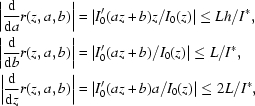since for real data, i.e. .

Then redefine the function ,

If the variable is fixed, then the new function has all the properties described above. Since

then on the whole image one can find for the pairs , where a = and b = , j = .

2.2.2. A method to find the stretch factors

So far we have supposed that the pairs are known. Now we discuss how to find them. Assume that there is an area , where . This means that there is an area where the detector is relatively free of dust, dirt or other perturbing influences or where the intensity could be easily corrected. For example, the structures seen in the top right part of Fig. 2 ▶ could be successfully decreased after applying a median filter (Gonzalez & Woods, 2008 ▶). So one may assume that there is an area where = .

Suppose that there are constants , , , such that, at any moment of time , , . The following is usually true in practice: there is a region inside in which = 1 at a given point . In region , = and = . For convenience, should not be close to the edges of the images so, for any point , numbers and , the point .

Choose pairs , k = , , . Note that there is no correspondence between and or , i.e. the real values of and when the th white-field image or the th projection were acquired, and are still unknown. Let us introduce uniform grids on and with and grid points, so K = . We are going to determine and from .

Let us take an area inside and compare the functions

with the function

for , defined on . In practice we have noticed that several vertical segments in the images can usually be taken as . These segments are chosen in such a way so that have significant intensity fluctuations and these functions are easy to distinguish for different pairs . The accuracy of determining these pairs will be better when the profiles of are different on different segments belonging to .

We calculate for each and find the corresponding standard deviations on . The optimal is found when the minimal standard deviation is obtained. In the ideal case, the optimal corresponds to the zero deviation. In practice, however, the standard deviation corresponding to the optimal is typically non-zero.

2.2.3. Correction of intensity profiles

After the coefficients and , j = , have been identified for all white-field images, the function can be found for pairs , j = . For any of these pairs one can find and therefore , where = 1/a, = [see equation (11)]. So can be identified for new pairs of , i.e. is found for pairs in total. In a similar way one can identify for other pairs if equation (12) is applied. So there are pairs. And again one may use equations (11) and (12) to identify for other pairs , and so on. Suppose is found for some number of pairs . Based on the smoothness of one may expect that the found functions allow one to find for all i = with a good accuracy.

Some of these pairs may have similar values. Strictly speaking, a good approximation cannot be guaranteed if a given is far away from the known pairs. However, the white fields taken evenly during the data acquisition guarantee that the modes of the beam motion are well sampled. The authors expect the set of pairs found in the above manner can cover pairs for all projections. This is indeed verified in our experimental data processing. In principle, if the pair for one projection is out of the range of all pairs , one can always perform a calculation with equations (11) and (12) on a subset of the identified functions to extend the definition range of the pairs.

A similar approach can be used to find . In this case an area , where = 1, should be selected. Then is compared with the identified functions on . Once and are found, then

on .

2.3. A general case

In the above, the multiplicative function in equation (3) is assumed to be time independent, which is not strictly true. Here, possible vibrations in the optical detection system are taken into account, which comprises the scintillator, the objective and the CCD camera. Assume the following time-dependence,

This means that is shifting the imaging relative to the CCD camera along with the time. Let us also set = 0,  = 0.

In this paragraph white-field images are considered; projections can be corrected in a similar way. We have found that the vector in the experimental images is usually just a fraction of a pixel in magnitude. Let us choose an area , where is almost a constant along each horizontal segment belonging to . Taking various pairs we shift along the vector to obtain an image and find the quotient . Then the mean value and the standard deviation are found on each horizontal segment. The goal is to minimize the sum of all these standard deviations. Suppose the minimal summation is obtained at = and = . is therefore defined as . Instead of in the simplified case, should be employed to find in this general case. Similarly, can be found for each projection image, which is then employed to find .

3. Applications and discussion

3.1. Sample 1: plant stem Salix variegata

In order to assess the new method we examine the data collected for the plant stem (Salix variegata) and compare it with two other techniques. For the first technique we select one white-field image [assume it is ] and set by the following formula,

for i = [compare with equation (17)], i.e. we have assumed that . We refer to this as the one-slice correction method.

For the second technique, here referred to as the intermittent correction, each projection is corrected by the formula

where is the last white-field image taken before the projection under consideration.

Sinograms obtained by applying these established methods as well as the new method are shown in Fig. 6 ▶. The corresponding images reconstructed by a filtered back-projection algorithm (Natterer & Wübbeling, 2007 ▶) are shown in Fig. 7 ▶.

Figure 6.

A sinogram for a horizontal slice of a piece of Salix variegata. The one-slice correction (a), the intermittent correction (b) and the adaptive correction (c) are applied.

Figure 7.

The reconstructed slice of the plant stem using (a) the one-slice correction, (b) the intermittent correction and (c) the new adaptive correction.

Unsurprisingly, the one-slice correction gives the strongest ring artefacts. However, the intermittent correction also shows significant ring and wave artefacts in both the sinogram and the reconstructed slice. To compare these three techniques some metric characterizing the quality of artefact suppression is needed.

For all the projections we could find the rectangular region where there is only a white field, i.e. the stem does not project onto this rectangle. In the case of an ideal correction we should obtain = 1 for this rectangle. The variation in the standard deviation of inside the rectangle is plotted in Fig. 8(a) ▶. Taken over all the projections the average standard deviations for three techniques are: = 0.0185, = 0.0142, = 0.0068. Note that we take the rectangle (rather than ) since for some projections we have to shrink and shift the reference white field and we have no information about values of outside . As a result the correction will be definitely worse than inside the rectangle .

Figure 8.

A standard deviation of inside the rectangle as a function of projection number. The one-slice correction (blue line, A), the intermittent correction (red line, B) and the adaptive correction (green line, C) are applied. In (a) no filter and in (b) the mean filter was used.

While these deviations clearly demonstrate a better performance of our algorithm they do not quantify the ring artefacts. To obtain an indication of this we apply a median filter, which suppresses short-range fluctuations, e.g. those caused by vibrations in the optical system, which cause ring artefacts (see Fig. 8b ▶). As the sample does not project into the rectangle , the obtained standard deviations fully characterize the quality of wave artefact suppression. In this case = 0.0164, = 0.0115, = 0.0036. So some wave artefacts still persist (see also Fig. 9 ▶ and compare with Fig. 3 ▶, where the one-slice correction is applied) but are decreased by approximately three to four times in comparison with conventional flat-field correction methods.

Figure 9.

A projection cleaned by the adaptive technique.

The coefficients and are shown in Figs. 10 ▶ and 11 ▶. The absolute values of the vector are shown in Fig. 12 ▶. In this case the sample vibrations give only a subpixel shift.

Figure 10.

The magnification scale coefficient identified for each projection.

Figure 11.

The illumination shift coefficient (in pixels) identified for each projection.

Figure 12.

The absolute value (in pixels) of the detector shift of as a function of projection number.

The behaviour of the functions and can be explained in the following way. A user chooses the energy value, then the system sends pulses to motors controlling the position of components of the monochromator, so that only rays of the given energy penetrate a sample. Owing to thermal processes and vibration the positions of the components change over time. Once one component has changed its position too much, the system sends a pulse to the corresponding motor in order to return the component to the predefined position. Unfortunately, (i) each motor has a certain resolution, (ii) to return to the original energy it requires moving several components, (iii) some time is needed to stabilize the system. In addition, we have assumed that each image is acquired during a very small time. However, to take one image we need to expose the CCD during some time (in our cases it often varies from 300 to 600 ms), which is more than a ‘period’ of vibrations on the monochromator. Therefore but

The CoolSNAP-K4 camera used at the beamline allows us to acquire at most three frames per second, so we cannot determine how the real white field depends on time. In addition, decreasing the exposure time does not help, since the signal-to-noise ratio of the CCD sensor decreases and the time between frames cannot be decreased to zero. Another possibility is to use an ultra-fast CMOS camera, but this will not help since both the flux of the X-ray beam available at the beamline and the signal-to-noise ratio of the CMOS sensor will not allow us to sufficiently improve the intensity resolution over time.

After we have acquired a set of white fields with 50 ms exposure time and about 300 ms between shots we may only suppose that the real intensity profile has some ‘period’ (less than a second) depending on the time needed to stabilize the system. Note that there is no ‘periodicity’ for and as one may suggest from Figs. 10 ▶ and 11 ▶ (e.g. when images’ numbers are greater than 700): we have checked other data sets.

3.2. Sample 2: zebrafish Danio rerio

Now we consider a sample where the structure and the background have similar attenuation coefficients, so it is difficult to separate them when additional artefacts appear. The sample is a zebrafish Danio rerio. The same projection before and after the correction proposed in the paper is shown in Fig. 13 ▶; the reconstructed slice and region of interest are shown in Fig. 14 ▶.

Figure 13.

Zebrafish (Danio rerio): (a) the original projection, (b) the same projection after the proposed method has been applied; the dashed line indicates the position of the slice reconstructed in Fig. 14 ▶.

Figure 14.

Zebrafish (Danio rerio): (a) full area and region of interest (inset), (b) one-slice correction, (c) linear interpolation between white fields, (d) the proposed method, (e) and (f) additional ring artefact suppression described by Titarenko et al. (2010 ▶) is applied to (c) and (d).

We also used a linear interpolation of white fields in order to correct the ring artefacts, (see Fig. 14d ▶). The method suppresses the ring artefacts well only near several rays; the angle between the rays is about = 12°. This is due to the fact that only projections acquired just before or after a white field has been taken are cleaned well using the standard flat-field correction technique with the corresponding white-field image. The method proposed in the paper also does not suppress all artefacts (see Fig. 14e ▶); however, the method makes the artefacts more ‘regular’, i.e. their strength depends weakly on the polar angle. As a result, additional pre-processing based on the method of Titarenko et al. (2010 ▶), which is developed for suppression of ‘regular’ ring artefacts, allows us to see the difference between the proposed method and the method based on linear interpolation more clearly.

Now we discuss practical considerations for implementing the method proposed in the paper and possible ways to improve the method. Firstly, let us discuss suppression of wave artefacts caused by shrinking and shifting the incident X-ray beam in the vertical direction. To correct intensity profiles we just choose one to three vertical line segments (their height is about 90% of the projections’ height), so that a sample is never projected onto these segments during acquisition. Since the number of segments is small we often choose them manually, so they cross as many ‘hills’ as possible on the intensity profile. Note that the method cannot be used if the sample’s shadow is larger that the image sensor. In principle the lines should not be the same during acquisition. For example, if a sample’s horizontal cross sections are elongated, then one may choose fewer but better distributed vertical segments, i.e. where the number of ‘hills’ on the intensity profile is increased and these ‘hills’ are better separated, when the area covered by the sample’s shadow is minimal and increase the number of vertical segments when the shadow is wide. As we mentioned above, shrinking/shifting of the intensity profile is random. Therefore, if the number of white fields is small, e.g. <5, then it may happen that the shrinking/shifting factors , , j = , have similar values, which are far away from the factor , , i = , found for projections. Hence to find it may be required to apply a large number of operations described by equations (11) and (12) to the known functions . However, increasing the number of these operations causes additional errors in , since are known only for discrete values of and some interpolation is required. As a result, sometimes it is better to acquire an additional set of white fields, e.g. 100 images after the scan, and select those images having sufficiently different values of , .

Secondly, let us consider ring artefacts. We have assumed that the multiplicative function can only be shifted along a vector [see equation (18)]. However, when a scintillator/optics/CCD has been used for a long time, some radiation damage occurs and the time-dependence of may be written as

where is related to a ‘stable’ component, e.g. a CCD, optical system and scintillator, and is determined by a ‘moving’ component, e.g. a monochromator. In the case of a clean undamaged optical system, the number of small ‘features’ similar to those shown in the inset of Fig. 2 ▶ is very small, therefore is a very smooth function and ≃ if a point is near , so we may use equation (18). This is true for the first sample (plant stem Salix variegata). However, if the radiation damage is high and there are a lot of dust/dirt/scratches on the surfaces of the optical system, the number of ‘features’ for is increased. Unfortunately, proper determination of is not always possible, therefore shifting the original white field along the vector to find and the ratio as described in §2.3 will suppress ring artefacts caused by the ‘moving’ component but introduce new artefacts caused by shifting the ‘stable’ component . This is true for the zebrafish sample. To overcome this problem the authors will propose a method to separate and in a forthcoming paper, so that the method will also be applicable for damaged optical systems.

4. Conclusions

The proposed white-field correction method based on a continuous adaptive correction using intermittent white-field measurements effectively suppresses both ring and wave artefacts. The time required to process a volume depends on the sizes of the areas and number of temporary images used in the method. However, to obtain enough suppression it takes less than 10 min spent on an ordinary Intel Dual-core processor. Further improvements are possible and will be discussed in future papers. For instance, ring artefacts could be better suppressed if a subpixel structure of the white-field image is found. This is possible in principle, since there are several white fields shifted on subpixel lengths. For remaining artefacts it would be possible to apply suppression algorithms based on sinogram smoothness (see, for example, Titarenko, 2009 ▶; Titarenko et al., 2009 ▶; Titarenko & Yagola, 2010 ▶). Wave artefact suppression could also be improved if the function is found for a greater number of pairs . While we have focused on parallel beam synchrotron data it should in principle be possible to extend the method to cone beam optics and other types of time variations that affect the white fields collected during acquisition. Finally we should mention that the proposed adaptive correction technique is based only on two types of motion. The next steps should take into account instability of the intensity profile of the beam during acquisition, as well as possible beam-hardening and diffraction effects.

References

- Boin, M. & Haibel, A. (2006). Opt. Express, 14, 12071–12075. [DOI] [PubMed]
- Chu, Y. S., Liu, C., Mancini, D. C., De Carlo, F., Macrander, A. T., Lai, B. & Shu, D. (2002). Rev. Sci. Instrum.73, 1485–1487.
- Davis, G. R. & Elliott, J. C. (1997). Nucl. Instrum. Methods Phys. Res. A, 394, 157–162.
- De Carlo, F. & Tieman, B. (2004). Proc. SPIE, 5535, 644–651.
- De Carlo, F., Xiao, X. & Tieman, B. (2006). Proc. SPIE, 6318, 63180K.
- Gonzalez, R. C. & Woods, R. E. (2008). Digital Image Processing, 3rd ed. New Jersey: Pearson Prentice Hall.
- Hsieh, J., Gurmen, O. E. & King, K. F. (2000). IEEE Trans. Med. Imag.19, 930–940. [DOI] [PubMed]
- Münch, B., Trtik, P., Marone, F. & Stampanoni, M. (2009). Opt. Express, 17, 8567–8591. [DOI] [PubMed]
- Nakayama, K., Okada, Y. & Fujimoto, H. (1998). J. Synchrotron Rad.5, 527–529. [DOI] [PubMed]
- Natterer, F. & Wübbeling, F. (2007). Mathematical Methods in Image Reconstruction, Vol. 5, SIAM Monographs on Mathematical Modeling and Computation. Philadelphia: SIAM.
- Niederlöhner, D., Nachtrab, F., Michel, T. & Anton, G. (2005). Nucl. Sci. Symp. Conf. Rec.4, 2327–2331.
- Raven, C. (1998). Rev. Sci. Instrum.69, 2978–2980.
- Sadi, F., Lee, S. Y. & Hasan, M. K. (2010). Comput. Biol. Med.40, 109–118. [DOI] [PubMed]
- Sijbers, J. & Postnov, A. (2004). Phys. Med. Biol.49, N247–N253. [DOI] [PubMed]
- Smith, A. D., Flaherty, J. V., Mosselmans, J. F. W., Burrows, I., Stephenson, P. C., Hindley, J. P., Owens, W. J., Donaldson, G. & Henderson, C. M. B. (2006). Proceedings of the 8th International Conference on X-ray Microscopy, IPAP Conference Series, Vol. 7, pp. 340–342.
- Stock, S. R. (2008). MicroComputed Tomography: Methodology and Applications. CRC Press.
- Titarenko, S. (2009). British Applied Mathematics Colloquium 2009, p. 102. University of Nottingham, UK.
- Titarenko, S., Titarenko, V., Kyrieleis, A. & Withers, P. J. (2009). Appl. Phys. Lett.95, 071113.
- Titarenko, S., Titarenko, V., Kyrieleis, A. & Withers, P. J. (2010). J. Synchrotron Rad.17, 540–549. [DOI] [PubMed]
- Titarenko, S. & Yagola, A. G. (2010). Moscow Univ. Phys. Bull.65, 65–67.
- Tucoulou, R., Martinez-Criado, G., Bleuet, P., Kieffer, I., Cloetens, P., Labouré, S., Martin, T., Guilloud, C. & Susini, J. (2008). J. Synchrotron Rad.15, 392–398. [DOI] [PubMed]
- Walls, J. R., Sled, J. G., Sharpe, J. & Henkelman, R. M. (2005). Phys. Med. Biol.50, 4645–4665. [DOI] [PubMed]
- Wang, Y., De Carlo, F., Mancini, D. C., McNulty, I., Tieman, B., Bresnahan, J., Foster, I., Insley, J., Lane, P., von Laszewski, G., Kesselman, C., Su, M.-H. & Thiebaux, M. (2001). Rev. Sci. Instrum.72, 2062–2068.
- Yang, J., Zhen, X., Zhou, L., Zhang, S., Wang, Z., Zhu, L. & Lu, W. (2008). The 2nd International Conference on Bioinformatics and Biomedical Engineering, pp. 2386–2389. IEEE.