Adapting internal statistical models for interpreting visual cues to depth

Abstract

The informativeness of sensory cues depends critically on statistical regularities in the environment. However, statistical regularities vary between different object categories and environments. We asked whether and how the brain changes the prior assumptions about scene statistics used to interpret visual depth cues when stimulus statistics change. Subjects judged the slants of stereoscopically presented figures by adjusting a virtual probe perpendicular to the surface. In addition to stereoscopic disparities, the aspect ratio of the stimulus in the image provided a “figural compression” cue to slant, whose reliability depends on the distribution of aspect ratios in the world. As we manipulated this distribution from regular to random and back again, subjects’ reliance on the compression cue relative to stereoscopic cues changed accordingly. When we randomly interleaved stimuli from shape categories (ellipses and diamonds) with different statistics, subjects gave less weight to the compression cue for figures from the category with more random aspect ratios. Our results demonstrate that relative cue weights vary rapidly as a function of recently experienced stimulus statistics, and that the brain can use different statistical models for different object categories. We show that subjects’ behavior is consistent with that of a broad class of Bayesian learning models.

Introduction

One of the biggest puzzles in perception is how the brain reliably and accurately estimates properties of the world from ambiguous sensory information. In vision, ambiguity arises from the projection of the three-dimensional (3D) world into a two-dimensional (2D) retinal image and from neural noise in sensory signals. Nevertheless, we seem to accurately and reliably perceive our world. The resolution of the apparent contradiction is that our world is highly structured – only few of the many possible interpretations of an image are reasonably likely. By incorporating prior knowledge of these regularities into perceptual computations, the brain can resolve much of the apparent ambiguity.

Bayesian decision theory provides the standard, normative framework for modeling the effects of prior knowledge on perception (Knill & Richards, 1996). The focus of most Bayesian modeling of human perception has been on estimating what internal statistical model the brain uses to make perceptual inferences (Sun & Perona, 1998; Mamassian & Goutcher, 2001; Geisler, Perry, Super, & Gallogly, 2001; Weiss, Simoncelli, & Adelson, 2002; Stocker & Simoncelli, 2006; Knill, 2007a). However, statistical regularities vary considerably between different object categories (e.g. coins are more likely to be perfect circles than brooches) and environments (e.g. perfect right angles are more likely in an office environment than in a forest). On a typical day, observers encounter objects from different categories and move between environments with different statistics. This suggests that the fundamental problem for Bayesian models of perception may not be what internal statistical models are embodied in perceptual mechanisms, but rather how the brain adapts and/or changes its internal models to match changing scene statistics.

Here, we focus on the role that internal models of scene statistics play in cue integration. The experiments are motivated by the observation that the reliability of a cue that relies on statistical regularities in an object property depends on how variable that property is in the environment; thus, the relative influence of that cue on perceptual judgments should depend on internalized models of that variability. Our earlier work has shown that when the variability of figure shapes in a stimulus ensemble is increased, subjects adapt to reduce the influence of the figural compression cue to surface slant relative to binocular cues on their slant judgments (Knill, 2007a).

The experiments presented here address three primary questions:

1. Can the brain adapt different internal statistical models of figure shape for different figure categories and effectively switch between them when interpreting stimuli drawn from the different categories?

2. Are there limits to the categorical dimensions that support this kind of model switching?

3. How rapidly are internal models adjusted to match changes in environmental statistics?

The results show that the internal statistical models needed to interpret figural compression are quickly changed to match the statistics of the shapes used as stimuli and flexibly applied when statistics differ between object categories. We describe a family of Bayesian models that can account for these effects and fit well with the experimental data.

Methods

Apparatus and calibration

Stimuli were presented in stereo on an inverted monitor (118 Hz, 1280 × 1024 pixels) whose image was viewed through a mirror. In Experiments 1–3, the mirror was horizontal, so that the virtual image of the monitor was also horizontal, building an angle of about 130° with subjects’ line of sight, which was pointed downwards by about 50°. In Experiments 4 and 5, the mirror was slanted so that the screen plane appeared fronto-parallel to the subject at an effective viewing distance of about 60 cm (see Figure 1). Subjects’ head position was fixed by a combined chin and forehead rest, and they viewed stimuli binocularly through StereoGraphics CrystalEyes active-stereo shutter glasses (RealD, Beverly Hills, CA) at a refresh rate of 118 Hz (59 Hz for each eye’s view). The two eyes’ views differed slightly from each other, and the resulting disparities created a vivid 3D impression of the stimuli. Black occluders on the mirror hid any part of the monitor frame that would otherwise have been visible to the subject. Stimuli were shown against a dark red background and drawn in different shades of red, using only the comparatively faster red phosphor of the monitor in order to minimize “ghosting”.

Figure 1.

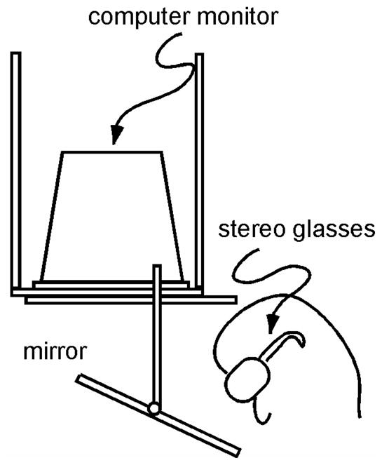
Experimental apparatus. Stimuli were rendered stereoscopically on an inverted monitor and viewed by the subject through a mirror, so that the virtual image of the monitor appeared below the mirror. The mirror was horizontal in Experiments 1–3, so that the virtual image of the screen was horizontal, too, and slanted as shown here in Experiments 4 and 5, so that the virtual image of the screen was fronto-parallel.

At the beginning of each experimental session, we calibrated the virtual environment by computing the positions of the subject’s eyes relative to the virtual image of the monitor. This allowed us to accurately render stereoscopic stimuli. The calibration procedure has been described previously (Seydell, Trommershäuser, & Knill, 2008). In it, subjects viewed the monitor monocularly with each eye through a half-silvered mirror and moved a physical probe on a table underneath the mirror to visually match test points displayed on the monitor. They matched the test points twice, using physical probes mounted at two different heights above the table. An Optotrak 3020 system recorded the 3D positions of the probe at each test location, and these data were used to compute the 3D positions of the subject’s eyes relative to the screen.

Stimuli and procedure

Subjects’ task in all experiments was to use the computer mouse to adjust a virtual probe to be perpendicular to the surface of a virtual slanted figure. Figures were either elliptical or diamond-shaped and were textured with small dots to provide subjects with rich disparity information about slant (see Figure 2). The dots were randomly positioned and shaped to minimize texture cues. A three-dimensional cylindrical probe extended away from the center of the surface. Subjects used the computer mouse to adjust the orientation of the probe to appear perpendicular to the surface, at which point they indicated a match by pressing the mouse button. The orientation of the probe judged to be perpendicular to the surface provided an implicit measure of the perceived orientation of the surface. We mapped movement of the mouse to rotation of the probe tip such that the axis of rotation was perpendicular to the direction of the mouse’s movement and in the horizontal plane, and the angular velocity was set proportional to the speed of the mouse.

Figure 2.

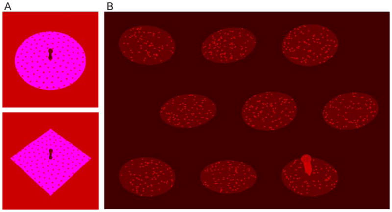
Stimuli. In all experiments, subjects viewed stimuli binocularly and used the computer mouse to adjust a virtual probe to be perpendicular to a slanted virtual surface. (A) Experiment 1 used ellipse and diamond stimuli, presented at screen center. Experiments 2 and 3 used ellipse stimuli drawn in purple and pink. Of the 146 stimuli presented per experimental block, 96 were “context stimuli” that could either all have an aspect ratio of 1 or have random aspect ratios. The remaining 50 stimuli were “test stimuli” used to calculate the relative influence of the compression cue on subjects’ slant judgments. Test stimuli contained ±5° cue conflicts between the slant suggested by the compression cue under the assumption that the figure has an aspect ratio of 1 and the slant suggested by stereoscopic disparities. (B) In Experiment 4, 9 ellipses, slanted at different angles, appeared at the same time in the display. The probe appeared consecutively on all ellipses. Of the 9 ellipses, 7 were context stimuli. In half of the trials (regular context), they were slanted circles, in the other half (random context), they were slanted ellipses with random aspect ratios. The remaining 2 ellipses were test stimuli. Subjects adjusted the probe for 5 of the context stimuli first and then for the remaining 2 context stimuli and 2 test stimuli in random order. In Experiment 5, the stimuli that were on the screen at the same time in Experiment 4 appeared sequentially. (Note: As it becomes evident particularly from the image of the slanted square diamond in Figure 2A, there are other figural cues (apart from the compression cue) that can be used to infer slant. For example, the distance from the base of the probe to the top vertex of the diamond is smaller than that to the bottom vertex. Under the (constrained) prior assumption that the figure is symmetric about its two main axes and the probe base coincides with surface center, the ratio of these distances provides a perspective ratio cue to slant. Similarly, changes in random dot density provide a texture cue to slant. In our stimuli, the slant suggested by these other perspective cues is always consistent with the slant suggested by the compression cue. Thus, what we refer to as “influence of the compression cue” is really an indicator of how strongly subjects rely on all figural cues, not just the compression cue. There are two reasons to assume that the compression cue dominates the other cues. First, with the stimuli and slants used, changes in slant lead to much larger relative changes in the aspect ratios of figures than in the other cues (e.g. at the small stimulus sizes used in Experiments 4 and 5, the aspect ratio of a circle displayed at 35° slant is 5.7% larger than the aspect ratio of a circle projected at 40° slant, while the perspective ratio changes by only 0.5%. At the larger stimulus sizes in Experiments 1–3, the perspective ratio still changes by only 1.7%). Second, previous studies suggested that in the kinds of displays used here, the visual system gives much more weight to the aspect ratio cue than to these other cues. Studies of slant from texture for random dot textures showed that texture density contributes minimally to slant judgments (Knill, 1998a,b,c). In another study (Knill, 2007a) using the same elliptical stimuli as in Experiments 1–3, but in which cue conflicts were constructed such that the other perspective cues agreed with the disparity cues, subjects gave almost as much weight to the compression cue alone as found here for the combination of figural cues.)

The stimuli contained two major cues to surface slant. The first cue, which we will refer to as the disparity cue, was the gradient of stereoscopic disparities across the surface. The second cue was provided by the shape of the figure as projected onto the subject’s retinas. Because there is a systematic relationship between the “true” aspect ratio of a figure in the world, the figure’s 3D orientation relative to the viewer, and the aspect ratio of the image of the figure as projected onto the viewer’s retinas, the 3D orientation of the figure can be inferred from the image aspect ratio, provided that the true aspect ratio is known or assumed. (For details, refer to Equation A3 in Appendix A.) For example, if a coin (which is known to have a true aspect ratio of 1) projects to an ellipse with an aspect ratio of 0.7 on the observer’s retina, the observer can infer that the coin is slanted by about 45.6°. Humans have an “isotropy bias” – they tend to assume that the true aspect ratio equals 1, and that the apparent compression of the figure is a consequence of its being slanted. We thus refer to the image aspect ratio of a figure, interpreted under the assumption that the true aspect ratio equals 1, as the compression cue.

In all of the experiments except for Experiment 4, trials consisted of the following sequence: A slanted figure (ellipse or diamond) appeared at screen center, accompanied by the probe. Subjects adjusted the orientation of the probe until it appeared perpendicular to the surface and hit the mouse button to indicate a match. In Experiment 4, subjects were shown nine slanted ellipses simultaneously in each trial, but made slant settings for one figure at a time. In all experiments, the ensembles from which stimuli were drawn consisted of two types of intermixed stimuli.

Test stimuli were used to measure the influence of the compression cue (relative to the disparity cue) on subjects’ judgments. Test stimuli were constructed to have conflicts of −5°, 0° or 5° between the slant suggested by the disparity cue and the slant suggested by the compression cue. Slant was defined relative to the viewer such that stimuli with a slant of 0° would be fronto-parallel, and stimuli were slanted about a roughly horizontal axis. Given the viewing geometry, with subjects’ heads pointed down at approximately 50° (see Figure 1), stimuli with a slant of approximately 40° appeared parallel to the ground. One of the cues always suggested a slant of 35°. The resulting pairs of slant suggested by the two cues were [35°, 30°; 30°, 35°; 35°, 35°; 35°, 40°; 40°, 35°]. To create conflicts, circles and square diamonds were distorted such that when projected from the slant specified for the disparity cue, they projected to the figure shape in an imaginary cyclopean eye midway between a subject’s two eyes that a circle or square diamond would have projected to were it slanted at the angle specified by the compression cue slant. Thus, for example, an elliptical stimulus with a stereoscopic slant of 35° and a compression cue slant of 40° would be an ellipse with an aspect ratio of .935 rendered stereoscopically at a slant of 35°. This resulted in a stimulus that appeared as an ellipse in the frontoparallel plane with an aspect ratio of .766 (consistent with a circle projected from 40° slant) and with stereoscopic disparities suggesting a 35° slant.

Context stimuli (together with the test stimuli) implicitly defined the statistics of the local stimulus environment. Either all context stimuli were slanted figures with aspect ratios of 1 (regular context), or they had random aspect ratios between 0.5 and 1 (random context). Note that what we refer to here as “context” includes not only other stimuli present at the same time as the test stimulus – in fact, such a local context was only provided in Experiment 4 – but also the stimuli that temporally preceded the test stimulus. The area of all figures was held constant to match the area of the test stimuli containing no cue conflicts. Context stimuli were “spun” by a random angle between 0° and 180° and were then rotated around a roughly horizontal axis by a slant randomly chosen from a fixed set of slants (these varied slightly between experiments). Depending on the experiment, between 65.75% and 77.78% of the stimuli were context stimuli.

Experiment 1

In Experiment 1, stimuli included both ellipses and diamonds, in equal proportion. Example stimuli are shown in Figure 2A. No-conflict test stimuli were circles and square diamonds. The circles had a diameter of 12 cm, the squares a diagonal length of 12 cm (at the viewing distance used in all experiments, 1 cm corresponds roughly to 1° of visual angle). Test stimuli were created as described above. Test stimuli were slanted around a horizontal axis and context stimuli were slanted around a randomly chosen axis between 0° and 180°.

The probe used for Experiments 1–3 was a 2 cm long cylinder with a diameter of 0.5 cm. It had spheres attached to the top and bottom to eliminate monocular cues to line orientation that otherwise would have been provided by the projections of the circular cross-sections of the cylinder. On each trial, the initial orientation of the probe was chosen randomly from a uniform distribution on the sphere described by all possible probe orientations with the constraint that the angle between the surface normal and the probe could not be larger than 90° (so that the probe would not intersect the surface) and not smaller than 30° (so that it was never roughly perpendicular to the surface initially). The major cues to the probe’s orientation were the same as for the test and context stimuli; stereoscopic disparities and figure compression. The probe, however, was designed to minimize the opportunity to simply match figural cues on the probe to those in the stimulus. The intersection between the cylinder and the sphere at the bottom of the probe in Experiments 1–3 may have provided cues to the probe’s orientation, but these were weak due to the small size of the cylinder. Linear perspective cues created by the parallel edges of the cylinder were similarly weak cues given the small size of the probe. As subjects were free to move the probe around and look at it at various angles, they could get rich information about its orientation despite its relatively small size.

Subjects completed 5 sessions on consecutive days. During the first two sessions, all context stimuli had aspect ratios of 1 (circles and square diamonds), in sessions 3–5 the context stimuli of one shape category were presented with random aspect ratios, while those of the other category kept having aspect ratios of 1. For half of the subjects, who were randomly assigned to the random diamond group, context stimuli in sessions 3–5 consisted of diamonds with random aspect ratios and circles. For the remaining subjects, who formed the random ellipse group, context stimuli in sessions 3–5 consisted of ellipses with random aspect ratios and square diamonds. Context stimuli were randomly slanted at one of four angles away from the fronto-parallel; 20°, 30°, 40° and 50°.

Each experimental session consisted of 4 blocks of trials and took about 50 minutes, including the time needed for calibration. Each experimental block consisted of 146 trials; 24 (12 ellipses, 12 diamonds) for each of the context stimulus slants, and 10 (5 for each stimulus category) for each of the test slant pairs. Thus, context stimuli comprised 65.75% of the total stimulus set. Within each block, all trials were presented in random order.

Experiment 2

Experiment 2 was the color analog of Experiment 1. Rather than mixing ellipses and diamonds in the stimulus set, we mixed pink and purple ellipses (note: we had to avoid using the relatively slow green phosphor). All aspects of Experiment 1 remained the same, with color replacing shape as the feature distinguishing figures with random or regular statistics. In sessions 1 and 2, all context stimuli were circles, and in sessions 3–5, purple context stimuli were always circles, whereas pink context stimuli were ellipses with random aspect ratios.

Experiment 3

Experiment 3 replicated Experiment 2, but here we explicitly informed subjects that the pink ellipses were randomly shaped and the purple ellipses were all circles before each block of trials in sessions 3–5.

Experiment 4

In Experiment 4, rather than showing stimuli individually on each trial, nine stimuli were shown simultaneously, arranged in a 3 × 3 array (Figure 2B). Each figure’s center was in the fronto-parallel screen plane, and surface orientation was defined relative to a local coordinate system whose z-axis connected the center of the surface with the cyclopean eye, and whose x- and y-axes spanned a locally fronto-parallel plane perpendicular to the line of sight to the center of the figure. The x-axis was defined as the projection of the line connecting the subject’s two eyes onto the locally fronto-parallel plane. The y-axis was given by the cross-product of the x and z-axes.

The display in each trial contained 2 test stimuli and 7 context stimuli. In regular context trials, the context stimuli were slanted circles with a diameter of 5 cm, while in random context trials they were slanted ellipses with random aspect ratios between 0.5 and 1 whose area was matched to that of the circles. Context stimuli were randomly spun in the plane prior to slanting. The slant of each context stimulus was chosen randomly from the set [25°, 30°, 35°, 40°, 45°]. Test stimuli were generated to have cue conflicts as described above. The axis about which a stimulus was slanted (often referred to as the tilt axis) was randomly drawn from a uniform distribution between −20° and 20° away from the horizontal. The location of the test stimuli in the set was randomly determined. To ensure that subjects attended to the context stimuli within a display, subjects made slant judgments for 5 randomly chosen context stimuli first, followed by a random combination of the remaining 2 test and 2 context stimuli.

The probe used in the experiment differed slightly from that used in Experiments 1–3. Rather than having a sphere at its base, it had a 1 cm long cone, whose tip was positioned at the center of the figure. The probe’s initial orientation was chosen randomly with the constraint that the angle between the probe and surface normal was at least 20° and maximally 50°.

The experiment consisted of 4 50-minute sessions, each of which comprised 5 blocks of 10 trials each. Because there were 9 stimuli per trial, a total of 90 surfaces were judged per block. Of these, 70 were context stimuli, and 20 (2 for each slant pair) were test stimuli. The first session consisted entirely of regular context trials (all context stimuli were circles). In sessions 2–4, each block consisted of 5 regular and 5 random context trials, presented in random order. For a control group of subjects, all trials in all sessions were regular context trials.

Experiment 5

Experiment 5 replicated Experiment 4 but with the difference that while the probe was being adjusted on one of the 9 surfaces, all other surfaces were hidden from view, so that there was always only one stimulus on the screen.

Subjects

All subjects were volunteers from the University of Rochester community who received a payment of $10 per session. They gave their informed consent prior to testing and were treated according to the guidelines set by the University of Rochester Research Subjects Review Board, who approved the study. All subjects had normal or corrected-to-normal vision. Upon entering an experiment, each participant was first tested for normal stereo vision using the third (contoured circles) of the RANDOT stereo tests (Stereo Optical Co., Inc., Chicago, IL, USA). Only subjects with a binocular acuity of 40 seconds of arc or better were admitted to the study. All subjects were naïve to the hypotheses under investigation, and each subject participated in only one of the experiments.

We initially ran 15 subjects per experimental group, but upon inspection of the data decided to exclude subjects for whom unusually large standard errors made the cue weights estimated from their slant setting meaningless (see Data analysis). Where necessary, we ran additional subjects to make up for the excluded subjects or to balance the number of subjects in the different experimental groups.

Experiment 1 was completed by 34 subjects, 4 of whom were excluded from the data analysis for the reasons mentioned above. Of the remaining 30 subjects, 15 were in the random diamond group and 15 were in the random ellipse group. They ranged in age from 18 to 36, and 19 of them were female. Experiment 2 had 15 participants, 8 of them female, who ranged in age from 18 to 26. In Experiment 3, 4 of 16 subjects had to be excluded from the analysis. The remaining 12 subjects ranged in age from 18 to 40, and 6 of them were women. Experiment 4 had 31 participants, 3 of whom (2 in the experimental group, 1 in the control group) were excluded from the analysis because of high standard errors. There remained 14 participants in the experimental group and 14 in the control group. Their ages were between 18 and 32, and 19 of them were women. In Experiment 5, the data of 4 subjects had to be discarded because of high standard errors. The reported results are based on the data of 15 subjects (6 men) who were between 18 and 32 years old.

Data analysis

Prior to data analysis we filtered outliers by computing the average probe slant and tilt settings separately for each subject, session, and condition, iteratively excluding slant settings that differed more than 3 standard deviations from the mean slant. Subjects’ errors in tilt settings were well fit by a Gaussian with a mean of approximately 0° and a standard deviation of approximately 11°. We found no significant correlation between errors in tilt settings and slant settings, so that we ignored tilt in our analyses of the slant settings.

To evaluate the relative influences of the two cues (disparities and figural compression assuming an aspect ratio of 1) on subjects’ slant estimates, we regressed, separately for each subject and condition, the subject’s slant settings Ŝ for the test stimuli against the slants suggested by the two cues, using the following equation:

$$\widehat{S}=b(w_{\mathit{comp}}{S}_{\mathit{comp}}+(1-w_{\mathit{comp}})S_{\mathit{disp}})+c.$$ (1)

S_comp is the slant suggested by the interpretation of the figure as having a true aspect ratio of 1 (the circle or square interpretation), S_disp is the slant suggested by the gradient of stereoscopic disparities across the surface, and the constants b and c capture multiplicative and additive biases in the subjective points of equality between surface and probe slants; w_comp is a measure of the relative influence of the compression cue on subjects’ slant judgments. Fitting Equation 1 to subjects’ judgments is algebraically equivalent to fitting a linear model y = w₁x₁ + w₂x₂ + c to the data and then normalizing the weights to sum to 1.

We used resampling to compute standard errors on estimates of individual subjects’ weights, w_comp, separately for each condition: We randomly sampled the experimental trials and ran the regression described above to compute an estimate for w_comp. This was repeated 1,000 times, and the standard deviation of the resampled estimates of w_comp was used as the standard error of the estimate. The data of subjects whose standard errors on w_comp exceeded those of the remaining subjects in the group by a factor larger than 3 (for the subjects where this occurred, it always occurred in multiple conditions) were excluded from the computation of the group means.

Results

Experiment 1

Experiment 1 tested whether subjects can adapt and use different statistical models for qualitatively different shape categories to interpret figural slant cues. In particular, we tested the hypothesis that when placed in a stimulus context in which one type of figure (e.g. ellipses) always had the same or near to the same shape (circles) and the other type (e.g. diamonds) had highly randomized shapes, subjects would adapt so as to down-weight the compression cue for the randomized figures, but not for the figures with consistent shapes.

In the first two sessions, which served as a baseline, subjects made slant judgments for test stimuli randomly intermixed with context stimuli that all had an aspect ratio of 1 (circles and square diamonds). In the following three sessions, the 15 subjects in the random diamond group made slant judgments for test stimuli randomly intermixed with slanted circles and diamonds with random aspect ratios, whereas the 15 subjects of the random ellipse group made slant judgments for test stimuli randomly intermixed with square diamonds and ellipses with random aspect ratios. The test stimuli for both groups of subjects were exactly the same (small conflicts between the compression cue and stereoscopic cues around 35°).

Figure 3 shows a prototypical subject’s average slant settings for the test stimuli in session 2 (the last baseline session, panels A and C) and session 5 (the last session, panels B and D). This subject was in the random diamond group, so by session 5 had been exposed to several sessions in which context stimuli contained circles and randomly shaped diamonds. Figure 3 shows the subject’s average slant settings for two sets of test trials – trials in which the slant suggested by stereoscopic disparities was fixed at 35° and the slants suggested by the compression cue were 30°, 35° or 40° (black triangles), and trials in which the slant suggested by the compression cue was fixed at 35° and the slants suggested by the binocular disparities were 30°, 35° or 40° (gray triangles). The two groups of conditions share the no-conflict 35°/35° condition. The straight lines represent best fitting straight lines to the data. If a subject were to give equal weights to the two cues, the slopes of the best fitting lines would be equal (see Figure 3C). If subjects gave more weight to binocular disparities, the gray line would be steeper than the black line. The relative slopes of the two lines determine the relative weight given to the compression cue. Note that for this subject, the data stayed relatively constant for ellipses between sessions 2 and 5, with the exception that the overall additive bias in slant settings (constant c in Equation 1) decreased by about 2°, but that the relative slopes of the two lines changed markedly between sessions 2 and 5 for the diamonds, indicating that the subject gave less weight to the compression cue for diamonds after exposure to a large set of randomly shaped diamond context stimuli.

Figure 3.

Slant settings in test trials of Experiment 1. Average slant settings for a prototypical subject in Experiment 1. This subject was drawn from the random diamond group. Session 2 was the last baseline session in which all context stimuli were either circles or square diamonds. By session 5, the subject had seen a large number of context stimuli containing circles and randomly shaped diamonds. The data are organized so that black, upward pointing triangles represent test stimuli for which the slant suggested by binocular disparities was fixed at 35° and the slant suggested by the compression cue varied between 30°, 35°, and 40°. The best fitting regression line to this data shows how this subject’s slant settings changed as the slant suggested by the compression cue increased from 30° to 40° while the slant suggested by binocular disparities stayed fixed at 35°. Gray, downward pointing triangles represent the opposite conditions, in which the slant suggested by the compression cue remained fixed at 35° and the slant suggested by binocular disparities varied from 30° to 40°. If the cue suggesting different slants had no influence at all, the slope of the line would be 0. If both cues influence slant judgments equally, the slopes of the gray and black lines would be identical. This is approximately the case in panels A, B, and C, all of which represent test stimuli that were embedded with large numbers of context stimuli that had an aspect ratio of 1. Only in panel D is the slope of the black line significantly smaller than that of the gray line, indicating that only in this condition, where test diamonds were embedded with context diamonds that had random aspect ratios, the influence of the compression cue on the subject’s slant judgments was significantly lower than that of the disparity cue. The dashed lines in A–C show this subject’s mean slant settings for cue-consistent stimuli (stereoscopic images of circles or square diamonds) at 30, 35 and 40 degree slants. For the diamond figures in the fifth session (D), there were no such stimuli, since the context stimuli had random aspect ratios. The dashed line, therefore, represents the subject’s mean slant settings for context stimuli at 30 and 40 degree slants. The fact that the slope of the lines exceeds 1 even for no-conflict stimuli reflects a high multiplicative gain between stimulus slant ant the subject’s matching probe slant.

Included in Figure 3, panels A–C, are dashed black lines showing the subject’s average slant settings for cue-consistent stimuli (stereoscopic images of circles or square diamonds) at 30°, 35°, and 40° of slant. The dashed lines have a slope greater than one for this subject, and while there was a large amount of variability across subjects, subjects consistently showed a similar qualitative pattern. The average multiplicative gain (bias term b in Equation 1) was equal to 1.54 ± 0.09 (M ± SE) – see Appendix B for more details. While this could reflect overall biases in the perceived orientation of surface, it could also reflect biases in the perceived orientation of the probe, or in what is perceived to be orthogonal orientations between the two – the data do not allow us to distinguish biases arising from subjects’ slant percepts and those arising from the matching procedure.

Figure 4 shows average compression cue weights for subjects in the two groups calculated separately for ellipses and diamonds and for the two baseline sessions and the last two sessions. As can be seen in Figure 4A, the relative influence of the compression cue on the random diamond group’s slant judgments remained constant for ellipse test stimuli (t (14) = −0.041, p = .968), whereas it significantly decreased for diamond test stimuli (t (14) = 3.172, p = .007). For the random ellipse group (Figure 4B), the opposite pattern was observed; the influence of the compression cue did not change significantly for diamond stimuli (t (14) = 0.749, p = .440), but it decreased significantly for ellipse test stimuli (t (14) = 4.645, p < .001). In both groups, the influence of the compression cue changed significantly more for the shape category whose context stimuli were presented with random aspect ratios in sessions 3–5 (both t (14) ≥ 3.116, both p ≤ .008).

Figure 4.

Relative influence of the compression cue in Experiment 1. (A) For the random diamond group (N = 15), context ellipses were always circles whereas context diamonds had random aspect ratios in sessions 3–5. No difference was observed between subjects’ reliance on the compression cue in the first two (pre-learning) compared to the last two (post-learning) sessions for elliptical test stimuli. However, for diamond test stimuli, the influence of the compression cue was significantly lower in the last two sessions than in the first two sessions. (B) The opposite was true for the random ellipse group (N = 15), for whom the diamond context stimuli were always square, but the ellipse stimuli had random aspect ratios in sessions 3–5: There was no significant change in compression cue influence for diamond stimuli between the first two and the last two sessions, but the influence of the compression cue dropped significantly for ellipse test stimuli. In both groups, the compression cue weights changed significantly more for the shape category whose context stimuli had random aspect ratios in sessions 3–5. Error bars in this and all following figures indicate ± 1 SEM.

Figure 5 shows the data on a finer temporal scale, with weights computed separately for each of the five sessions. Since both groups showed qualitatively similar effects, we averaged the results of the two groups together, grouping conditions by whether the context stimuli were regular or had random aspect ratios. These data clearly show that the adaptation effect appears immediately in the first session containing random shapes (session 3) and the weights remain essentially unchanged thereafter. This is consistent with fast, shape category-selective changes in cue weights following exposure to a mixed collection of randomized and regular stimuli – at least on the time scale of a single session (50–60 minutes). That the measured cue weights do not decrease further in later sessions may result from an adaptive process that is so fast that subjects’ performance averaged over one session represents asymptotic performance or that subjects have to re-adapt to the experimental stimulus statistics in each session after exposure to the real environment between sessions. Experiment 5 takes up the question of the speed with which observers change their internal models.

Figure 5.

Relative influence of the compression cue in Experiment 1 as a function of session number. Compression cue weights are averaged across both groups. Stimulus conditions were grouped by whether or not the context stimuli within the group had random aspect ratios or were regular (circle or square diamond) in sessions 3–5.

Because the weights in Equation 1 are fitted to the “true” slants suggested by each cue, they are confounded with possible differences in the perceptual scaling of each cue. These could arise from biased computations of slant from each cue or from biases in low-level sensory feature measurements associated with each cue; for example, biases in measured aspect ratios in the retinal image. Since we are interested in adaptive changes over time, however, we can still use the changes in measured cue weights to probe adaptive changes in internal statistical models, as long as the perceptual scaling of each cue does not change with experience. While we have no independent means of assessing cue-specific perceptual scaling, several lines of evidence suggest that they do not change with training in the current experiment. The observation that subjects’ normalized cue weights do not change over sessions when the context remains constant (the regular context weights shown in Figure 5) suggests that the perceptual scaling associated with cue does not change simply with exposure to the stimuli and the task – at least not differentially. Statistical tests (see Appendix B) also show no significant change in the gain factor, b, in the regression model in Equation 1 between the first two sessions and the last two sessions, nor any interaction between session and the context associated with a stimulus shape (isotropic or random). Since the gain factor, b, in the regression model is equal to the sum of weights derived from a simple linear regression (Ŝ = w_comp S_comp + w_disp S_disp + c), we would expect differential changes in the perceptual scaling of the two cues to affect fitted values for b as well as the normalized cue weights. Thus, the fact that there are no significant changes in b is another reason to assume that the observed changes in cue weights were not caused by cue-specific changes in perceptual scaling.

Experiment 2

In Experiment 2, we tested the generality of subjects’ ability to selectively adapt shape priors for different object classes. We hypothesized that, since shape statistics naturally vary across different shape categories in our environment but are unlikely to vary across different colors, there would be no selective adaptation of shape priors for figures of different colors. We repeated Experiment 1 using only ellipses and replacing the ellipse/diamond distinction with a purple/pink distinction. While the pink context ellipses were always circles, the purple ones were presented with random aspect ratios in sessions 3–5.

As shown in Figure 6A, the results of Experiment 2 were fundamentally different from those of Experiment 1. Compared to baseline sessions 1 and 2, the influence of the compression cue was significantly lower in sessions 4 and 5 for both pink (t (14) = 4.176, p = .001) and purple (t (14) = 4.903, p < .001) stimuli, although only the purple context stimuli had random aspect ratios. The changes were not significantly different for the two color categories (t (14) = 1.153, p = .268). Instead of occurring selectively for differently colored stimuli, adaptation generalized across colors.

Figure 6.

Relative influence of the compression cue in Experiments 2 and 3. In these experiments, pink context stimuli were always circles, whereas purple ones had random aspect ratios in sessions 3–5. (A) In Experiment 2, subjects (N = 15) were not explicitly made aware that color and shape statistics were correlated. After learning, the influence of the compression cue on subjects’ slant judgments dropped significantly for both colors, and the difference in the decreases for the two colors was not significant. (B) In Experiment 3, subjects (N = 12) were told repeatedly from the beginning of session 3 that pink stimuli were always circles, whereas purple stimuli were randomly shaped ellipses. Again, the influence of the compression cue dropped significantly after learning for test stimuli of both colors, and the drop was not significantly different for the two colors.

Experiment 3

A possible interpretation of these results is that top-down knowledge of the category-contingency of figure shape statistics mediates the results of Experiment 1. Subjects might deliberately switch perceptual strategies when they are aware of the category-contingent statistics; for example, by adjusting the attention they give to compression and stereoscopic cues accordingly. While the category contingent statistics were immediately apparent to subjects in Experiment 1 (e.g., subjects in the random ellipse group often commented after session 3 that we had switched from showing all circles to some randomly shaped ellipses), they may not have detected the color-contingency in Experiment 2 (subjects’ spontaneous comments did not explicitly refer to color-contingent statistics). To control for high-level mechanisms mediated by explicit knowledge of statistical contingencies, we replicated Experiment 2 while repeatedly telling subjects in sessions 3–5 (before each block of trials) that the pink stimuli were always circles and the purple ones were ellipses with random aspect ratios. Even though subjects now reported awareness of the contingencies, the results (shown in Figure 6B) replicated those of Experiment 2. Subjects’ reliance on the compression cue dropped significantly for both pink (t (11) = 9.758, p < .001) and purple (t (11) = 3.744, p = .003) stimuli, and there was no significant difference between the decreases in the two categories (t (11) = 1.651, p = .127).

Experiment 4

The shape statistics of objects in the environment change not only across object categories, but also across different local environments (e.g. forest vs. office). An optimal observer would use context cues to determine the appropriate model to use when operating in different environments. Experiment 4 tested the hypothesis that subjects would use a more constrained model of shape statistics and hence rely more on figural compression as a cue to slant when test stimuli are presented in a visual context containing only circles than when the same stimuli are presented in a context of randomly shaped ellipses.

Figure 7A shows the relative influence of the compression cue, averaged across 14 subjects. In the first session (regular context trials only), the relative influence of the compression cue was near 0.5, indicating that subjects relied about equally on compression and disparity. The influence of the compression cue in regular context trials pooled across sessions 2, 3, and 4 was significantly lower (t (13) = 2.995, p = .010), indicating an effect of the globally more random stimulus context in those later sessions, where regular context trials were randomly interleaved with random context trials. As expected, the relative influence of the compression cue was also affected by local stimulus context. It was significantly lower in random context trials than in regular context trials of sessions 2, 3, and 4 (t (13) = 3.292, p = .006). Significant changes happened based upon only one trial’s worth of context stimuli, as evidenced by the fact that even if we discounted trials preceded by trials with the same stimulus context from the analysis, the relative influence of the compression cue still differed significantly (t (13) = 2.565, p = .023) between regular and random context trials of sessions 2, 3, and 4; the average influence of the compression cue in regular context trials preceded by one or more random context trials was 0.413 ± 0.047, whereas in random context trials preceded by one or more regular context trials it was only 0.315 ± 0.036.

Figure 7.

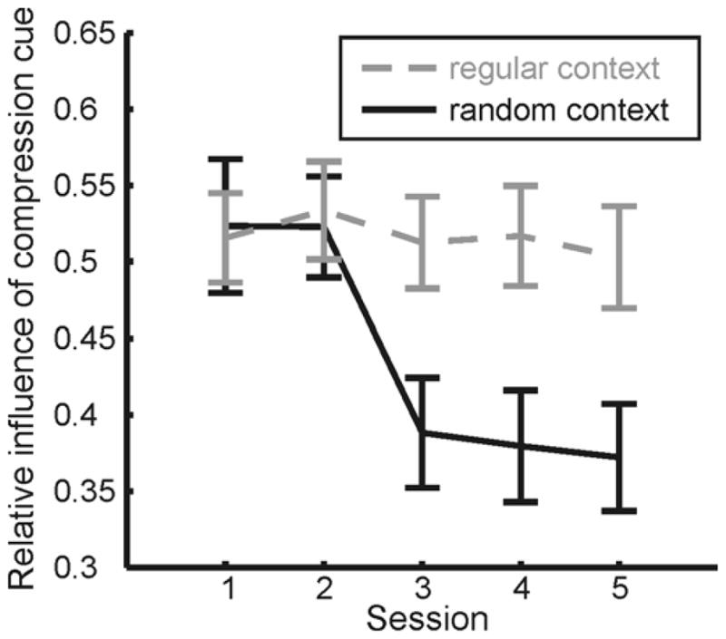
Relative influence of the compression cue in Experiments 4 and 5. (A) Results of Experiment 4, averaged over N = 14 subjects. Compared to a baseline measured in session 1 where the local stimulus context was regular on all trials, the influence of the compression cue was significantly lower in regular context trials of the last three sessions which were intermixed with random context trials. In addition, it was significantly lower in random context trials compared to regular context trials of sessions 2 to 4. No significant changes were observed in a control group of 14 subjects who viewed only regular context trials in all experimental sessions. (B) In Experiment 5, subjects (N = 15) made slant judgments for the same stimuli as in Experiment 4, but the 9 stimuli that made up a trial in Experiment 4 appeared sequentially. The influence of the compression cue was significantly higher for test stimuli embedded in a sequence of regular context stimuli than for test stimuli embedded in a sequence of random context stimuli, and highest in session 1, where there were only regular context stimuli.

A control group of 14 subjects who viewed only regular context stimuli in all sessions showed no significant changes in the influence of the compression cue on slant judgments between session 1 and later sessions (average decrease of w_comp: 0.002 ± 0.024, t (13) = 0.081, p (2-tailed) = .937); thus, the changes observed in the main experimental group were not simply due to repeated exposure to the experimental task.

Experiment 5

Experiment 4 was motivated by the question of how subjects adapt their internal statistical models of figure shape when they move between environments with different statistics. Theoretically, the brain might use the visual gist of the display (in our case, the context stimuli present at the same time as the test stimuli) as a cue to change the internal prior on shapes. Alternatively, the brain might rapidly adapt its internal model based on the sequence of stimuli viewed over time (i.e. the context stimuli temporally preceding the test stimuli, whether or not visible at the same time as the test stimuli). Experiment 5 was motivated partly by this question and partly by a desire inspired by the fast adaptation found in Experiment 1, namely, to measure how quickly subjects can adapt their internal models of shape statistics based on the history of stimuli viewed (in the absence of a local visual context).

Measuring the time course of changes in cue weights is a much more difficult experimental problem than measuring the time course of other types of adaptation in which a bias is introduced in a sensory stimulus or in a sensory-motor mapping (e.g., light adaptation, prism adaptation, saccade adaptation, etc.). In the latter case, one often induces biases that are significantly larger than the system noise, so one can track adaptive changes on a fast time scale. Here, we are constrained to use cue conflicts of a similar scale to the sensory noise (to avoid the non-linear down-weighting of cues found at large cue conflicts; Knill, 2007a). Moreover, cue weights must be computed by looking at slant settings for a range of conflict conditions in order to accurately account for additive and multiplicative biases in subjects’ judgments. The result is that one requires a large number of test stimuli to compute one set of weights. In our experiments, for example, the standard errors on estimates of individual cue weights from a one-hour session are on the order of 10–15% of the magnitudes of the weights.

A natural way to study the time course of adaptation when many test stimuli are needed to compute a set of weights is to present subjects with alternating sequences of regular and random context stimuli, each separated by test stimuli used to measure the resulting oscillations in cue weights. The resulting amplitude of oscillations in the weights is a measure of the gain of the system at the frequency of the alternating sequences. However, subjects might well detect the periodicity of the pattern and learn to quickly switch models at the appropriate frequency. Thus, it is better to present blocked sequences of regular and random context stimuli in random order. Therefore, we chose for Experiment 5 an experimental design equivalent to Experiment 4 with the modification that the 9 stimuli shown on a single trial in Experiment 4 were presented as a sequence of 9 single-stimulus trials. This has the further advantage of randomizing the time of presentation of test stimuli within a sequence to be two randomly chosen times in the last four stimuli of each nine-stimulus sequence.

The result is that subjects cannot easily detect the temporal structure of the stimulus sequences. The results of Experiment 5 almost exactly replicated those of Experiment 4. The influence of the compression cue was highest in the first session, significantly (t (14) = 2.420, p = .030) lower in the regular context sequences of later sessions, and again significantly (t (14) = 3.004, p = .009) lower in the random context sequences (Figure 7B). The result remained unchanged if we only looked at test stimuli preceded by a single sequence of “same”-context stimuli. The average influence of the compression cue in test stimuli preceded by a single sequence of regular context stimuli (itself preceded by one or more sequences of random context stimuli) was 0.397 ± 0.026, whereas the average influence of the compression cue in test stimuli preceded by one sequence of random context stimuli (itself preceded by one or more sequences of regular context stimuli) was 0.296 ± 0.037. These estimates differed significantly from one another (t (14) = 2.641, p = .019).

Discussion

Knill (2007b) showed that subjects adapt so as to give less weight to the figural compression cue relative to the disparity cue when test stimuli that deviate by small amounts from circularity are embedded in a larger stimulus set containing ellipses with broadly distributed, random aspect ratios. Operationally, the adaptations reflect themselves in the weights derived from a linear regression of subjects’ slant settings against the slants suggested by the compression cue and disparity cues, respectively. This should not be taken to mean that subjects are literally adapting cue weights. From a normative perspective, the apparent weight that an integrative process gives to the compression cue depends on two things – sensory uncertainty in the coding of figure shape (on the retina) and statistical assumptions about the distributions of shapes in the environment. Since we expect that sensory uncertainty in shape encoding does not change markedly when the statistics of viewed shapes changes, we interpret the adaptive changes as reflecting changes in subjects’ internal models of shape statistics to match the statistics of the environment (for more on this point, see the section on computational considerations below). Leaving for the moment the question of underlying mechanisms, we will refer to the adaptive changes observed experimentally as changes in subjects’ internal models of shape statistics, whether those internal models are explicitly represented in the nervous system or implicitly instantiated in integration and interpretation networks.

Category contingent adaptation

Experiments 1–3 show that the visual system can separately adapt and use different internal statistical models for qualitatively different shape categories (ellipses and diamonds), but not for different color categories (purple and pink). There are several partially related potential explanations for this. The fact that explicit knowledge of the contingencies did not aid selective adaptation in Experiment 3 indicates that the observed changes are driven by an implicit learning process. Michel and Jacobs (2007) proposed that perceptual learning operates on parameters of statistical contingencies between scene variables that are known to be dependent (parameter learning), but not on parameters describing contingencies considered a-priori independent; that is, for which a new contingency needs to be learned (structure learning). Similarly, several authors have suggested (e.g. in attempts to explain the McCollough effect; McCollough, 1965) that the visual system actively counters learning of correlations between stimulus dimensions (e.g., color and orientation) assumed to be uncorrelated, attributing any observed correlations to faulty calibration of the system (Dodwell & Humphrey, 1990; Bedford, 1995; Walker & Shea, 1974). In line with these considerations, the visual system may implicitly represent statistical contingencies between qualitative shape categories and shape statistics – for example by having mechanisms that support independently adapting statistical models for different shapes when appropriate – while having no such prior representation of continegencies between color and shape statistics. This aspect of our results resembles findings by Jacobs and Fine (1999). In their study, subjects estimating the depth of cylinders did not learn to rely differently on depth cues whose relative reliability was manipulated to be different for left-oblique and right-oblique cylinders, even though a pilot study showed that they could learn different cue weights for horizontal and vertical cylinders. Possibly, this occurred because in nature, horizontal and vertical objects are more likely to belong to different categories than left-oblique and right-oblique objects.

Speed of adaptation

The results of Experiment 4 seem to be at odds with the results of recent work (Muller, Brenner, & Smeets, 2009), in which subjects judged the slant of an ellipse surrounded by other ellipses that were either unambiguously isotropic or had random aspect ratios. Contrary to the authors’ expectations, subjects did not rely more on the compression cue in the former than in the latter condition, whereas in our Experiment 4 they did. The critical difference between the experiments is that our subjects judged slant for each context stimulus, whereas in Muller et al.’s study they did not. Rather, they had to ignore the distracting slant of the individual context stimuli in order to match the slant of the plane spanned by the centers of the context stimuli with the slant of the test stimulus. The results of Experiment 5 provide a resolution of the apparently conflicting results. In Experiment 5, subjects viewed and made slant settings for stimuli with the same temporal ordering statistics as in Experiment 4. This resulted in the same pattern of results observed in Experiment 4; thus, the changes in Experiment 4 seem likely to be due to rapid adaptations to the shape statistics of recently attended figures; rather than model switching based on context cues (as observed with the shape-contingent affects found in Experiment 1).

Experiment 5 demonstrates that subjects’ slant judgments for stereoscopically presented stimuli fluctuate rapidly as a function of the statistics of recently attended stimuli. When judging the slant of a test stimulus containing a 5° conflict between the slant suggested by stereoscopic disparities and by figural compression, subjects relied significantly more on the compression cue when the test stimulus was preceded by a small number of stimuli with aspect ratios of 1 than when preceded by a small number of stimuli with random aspect ratios. It takes surprisingly little evidence of a change in stimulus statistics to significantly change subjects’ shape priors. After observing a sequence of stimuli with one shape distribution (circles or random ellipses), it takes only 5–7 views of stimuli with different statistics for subjects to show adaptive changes to the new statistics. While Knill (2007b) has previously shown that subjects adapt their internal model of shape statistics based on the statistics of shapes in a stimulus ensemble, that paper did not analyze the time course of the change. In fact, Knill effectively assumed a relatively slow rate of adaptation by fitting subjects’ data with an exponentially decaying function over the weights derived from each session. The results of Experiment 5 show that the adaptation is very fast.

The finding that priors change rapidly based only on stimulus statistics (without feedback from a separate sensory cue like haptics) has important implications for experiments on cue integration in which the reliability of at least one of the investigated cues depends on prior assumptions that can either be more or less constrained. The latter is nearly always the case in visual depth perception, one of the most studied domains of sensory cue integration (to name only few of a large number of publications: Richards, 1985; Bülthoff & Mallot, 1988; Johnston, Cumming, & Parker, 1993; Curran & Johnston, 1994; Johnston, Cumming, & Landy, 1994; Landy, Maloney, Johnston, & Young, 1995; Jacobs, 1999; Fine & Jacobs, 1999; van Ee, Adams, & Mamassian, 2003). For example, humans tend to interpret monocular cues to surface shape and 3D orientation based on constrained priors such as symmetry, homogeneity, isotropy, rigidity, good continuation, Lambertian reflectance, illumination from a single, overhead, fixed light source, and many more. Whenever such a constrained prior competes with a broader one, stimulus statistics determine how strongly subjects rely on either prior. This in turn influences the observed cue weights, because it affects the variance of the inferred likelihood function, and thus the cue’s reliability.

Computational foundations of Bayesian adaptation

The results of Experiments 4 and 5 show that the influence of figural compression cues on subjects’ slant judgments changes on a fast time scale in response to changes in the shape statistics of stimuli being viewed binocularly. After viewing only a few randomly shaped, slanted ellipses, subjects’ slant judgments become less biased toward a circular interpretation of elliptical stimuli, even when that interpretation is close to the slant suggested by binocular disparities. After then viewing only a few slanted circles, subjects’ slant judgments become more biased toward a circular interpretation of those same test stimuli. Empirically, we have measured the bias toward circular (or isotropic) interpretations of stimuli using cue weights derived by regressing subjects’ estimates of slant against the slants suggested by the compression cue (under an isotropy assumption) and binocular disparity cues. The standard mode of discourse about cue integration, which implicitly assumes that cue integration happens by first estimating scene parameters independently using each cue and then computing a weighted average of the results, would lead one to posit adaptive mechanisms that explicitly adjust these weights based on stimulus information. In our view, this requires a premature jump to significant assumptions about mechanism that have no supporting evidence in the cue integration literature. While measuring different cues’ relative influences on psychophysical judgments using linear regression models is a reasonable way to derive summary measures of a system’s behavior, it does not imply a straightforward mapping between elements of the empirical model and the mechanistic structure of processes involved in cue integration. The data simply do not tell us about the underlying mechanisms.

Besides this philosophical reasoning, the strongest argument against a heuristic adaptation mechanism that directly adjusts a set of internal cue weights based on the statistics of stimuli viewed comes from experiments showing that a linear weighting scheme cannot account for how subjects combine figure shape and disparity information over a large range of cue conflicts (Knill, 2007a). Subjects appear to give less weight to the compression cue as conflicts grow. Subjects’ slant judgments from stimuli with a large range of cue conflicts are better fit by a Bayesian estimator that assumes that figures can be drawn from one of two categories – isotropic figures (e.g. circles) or figures with random aspect ratios. This observation leads us to model subjects’ adaptive behavior as adaptations of the parameters of such a model. The resulting model is not a mechanistic model, but rather a computational model in the sense that it describes the computational problem that observers are solving rather than the mechanisms they use to solve it. In a Bayesian model, an observer may modify two categories of parameters to adapt to environments with different statistics – parameters characterizing sensory noise and parameters characterizing the statistics of the environment. Both of these types of modification can lead to a system that empirically appears to “change cue weights” as stimulus statistics change. For reasons outlined below, we model subjects’ behavior in the current experiments as a result of adaptive changes in their internal model of environmental statistics.

Knill (2007b) described an adaptive Bayesian model that changes its internal model of figure shape statistics based on stimulus information to account for changes in cue weights based on the shape statistics of binocularly viewed figures. We describe a more general family of adaptive Bayesian models that can account for the kinds of fast adaptation shown here. Being normative models, these provide a framework for understanding the computational issues involved in the type of adaptation behaviors shown by subjects. We describe the basic elements and structure of the models, describe the constraints placed on the models by the data, and use these to draw inferences about the computational elements driving subjects’ behavior.

Figure 8 shows a cartoon diagram of an adaptive Bayesian estimator of surface orientation using both stereoscopic disparities and retinal figure shape. The key point is that the information provided by retinal figure shape depends both on sensory noise in the coding of shape information and on an internal model of the statistics of figure shapes in the environment. This model is particularly simple for ellipses. Since ellipses project to ellipses under perspective projection, a figure’s aspect ratio and orientation completely capture all the relevant information for slant judgments. If all elliptical figures in the world were in fact circles, the information provided by figure shape in the image would be limited only by sensory noise. In a world containing non-circular ellipses, the information is also shaped by the distribution of aspect ratios in the world; thus, in more random worlds, figure shape is a less reliable cue to surface orientation.

Figure 8.

Schematic diagram of an adaptive Bayesian model. The estimator relies on an internal model of shape statistics to interpret the retinal figure shape information. By combining noisy sensory information provided by disparities and retinal figure shape with prior knowledge of shape statistics, the estimator derives a probability distribution on the likely orientations and shapes that gave rise to the sensory data. In the model described in the text, the derived information about shape is used to update the internal model of the current statistics of shapes in the environment (dashed arrow).

The form of the estimation model is driven by experimental results on robust Bayesian cue integration (Knill, 2007a). Data from experiments measuring slant judgments for stimuli like those used here but with a range of cue conflicts show that a linear model of cue integration is a poor account of how subjects integrate figural compression cues and binocular cues to slant. In particular, subjects’ cue weights (derived from regression analysis applied to subjects slant estimates) vary smoothly as the conflict between the cues is increased – the relative influence of figural compression shrinks as the size of the conflict increases (Knill, 2007a). These data were well-fit by an optimal Bayesian estimator that assumes that figures are randomly drawn from one of two classes (figures with an aspect ratio of 1 – circle or square diamond, for example (we occasionally refer to these stimuli as isotropic, even though square diamonds are not isotropic in the sense that it is uniform in all directions) – or figures with random aspect ratios). Figure 9 shows a schematic diagram of the estimation model. The reported change in weights observed as a function of the size of cue conflicts reflects the degree to which stimuli are consistent with one or the other class of figures.

Figure 9.

Schematic diagram of the generative process assumed by the estimator used in the model. The estimator assumes that figures are drawn from one of two categories – isotropic figures (e.g. circles) or figures with a distribution of random aspect ratios. The figure seen at any particular instance is randomly drawn from one of the two sets with probabilities p_isotropic and 1−p_isotropic. If it is drawn from the random ensemble, its aspect ratio is presumed to be drawn from the appropriate probability distribution. The likelihood function for slant from the retinal shape information is an additive mixture of likelihood functions computed for each of the two sets of figures, weighted by the probability that a figure is drawn form each set. While the peak of the likelihood function is roughly coincident with the isotropic interpretation of the figure, the possibility that the figure is drawn from the random set gives the likelihood function long tails. The likelihood function for the combined cues (obtained by multiplying the two likelihood functions for slant from disparity and slant from retinal shape) is “pulled” toward the isotropic interpretation if the disparities are roughly consistent with the slant suggested by the isotropic interpretation, but is pulled less and less toward that interpretation the larger the conflict between the two. Similar likelihood functions can be derived for the shape of the figure. These can drive adaptive changes in the internal model (e.g. of the assumed mixture proportion p_isotropic).

Experience-dependent changes to any of the estimator parameters can result in changes in apparent cue weights (as measured experimentally). Candidate parameters include the variance of sensory noise on disparity and shape measurements, the relative proportions of figures drawn from the random and isotropic ensembles in the mixture model and the distribution of shapes in the random ensemble. We reject the hypothesis that observers in our experiments behave the way they do as a result of adaptive changes in their internal models of sensory noise for two reasons. First, to detect a change in cue weights of the magnitude that we see in the experiments from such adaptive changes would require that subjects change their estimates of the relative variance in sensory noise in shape and disparity measurements by between 80% (Experiment 1) and 120% (Experiments 4 and 5); that is, such a model would work by “learning” after exposure to randomly shaped figures that the variance in the sensory noise in its estimates of aspect ratios had approximately doubled or that the variance in the sensory noise of disparity measurements had approximately halved (or some equivalent combination of changes). Secondly, in Experiment 5, subjects would have had to adapt their estimates of internal noise by almost the same amount both up and down within 9 to 18 stimulus presentations. It is implausible that the true sensory noise changes in such a manner, and so we consider it implausible that the brain incorporates an internal of model of sensory noise that is so malleable.

This leaves as a candidate mechanism one that adapts or changes its internal model of the statistics of figure shapes as a function of the stimulus context. A model that accommodates optimal cue integration in the presence of frequent changes in scene statistics is well-suited to a non-stationary world, in which scene statistics might be expected to vary considerably across environmental contexts. In the model described so far, the adaptive changes in cue weights observed in our experiments could be due to changes either in the proportion of figures that are assumed to be isotropic or in the distribution of aspect ratios in the class of random figures. We can easily eliminate the latter as a candidate parameter for adaptation – simulations show that even very large changes in the distribution of random shapes within the random shape category (letting it go to infinity) cannot account for the decrease in compression cue weights observed. This is because our previous data (Knill 2007b) suggest a default model in which only a small proportion of figures are assumed to be random.

We are ultimately left with one parameter in the model that may be adapted – p_isotropic, the estimate of the prior probability that a figure in the world is isotropic. Changes in this “mixture proportion” can have a significant effect on the influence of the compression cue on subjects’ slant judgments. If the estimator assumes all figures are isotropic, the reliability of the compression cue (hence its perceptual weight) is determined entirely by noise on sensory estimates of the aspect ratio of a figure in the image. If the estimator assumes all figures are drawn from a random set of shapes, the reliability of the compression cue and its perceptual weight is determined by both the sensory noise and the assumed variability of aspect ratios in the world. Values in between give rise to weights in between those that would be found for an estimator assuming a purely isotropic model and those that would be found for an estimator assuming a purely random model. This is true even for figures that are close to being isotropic, for which the sensory data is reasonably consistent with an assumption of isotropy, because the estimator always takes into account the likelihood that the figure is not isotropic.

For an environment in which shape statistics change stochastically over time according to some well-specified dynamics, one can derive an optimal, adaptive Bayesian mechanism that will use the information provided by each stimulus not only to estimate slant, but also to update its internal model of the shape statistics. Since the mixture proportion of isotropic and random figures that characterizes the statistics of shapes in the environment changes stochastically over time, an observer cannot exactly know the true mixture proportion. It therefore maintains and updates an internal model that is a probability distribution over possible values for the mixture proportion, which is updated on each trial based on the history of stimuli viewed up to that point. The ideal observer for the slant estimation task goes through two processing steps on each trial (see Appendix A for details). The first is an adaptive step in which the observer updates its current internal model of the probability distribution over possible mixture proportions based on the stimulus information on that trial. The second step is an estimation step in which the ideal observer computes a probability distribution over possible slants given the current stimulus information and the current model of the probability distribution over mixture proportions. This is a slight extension of the ideal slant estimator that has complete knowledge of the parameters of the prior distribution of aspect ratios in the environment. In essence, it computes a set of probability distributions on slant, given the current stimulus information – one for each possible value of the mixture proportion (each possible prior on aspect ratios). It then computes the average of these probability distributions weighted by the current probability distribution on possible values for the mixture proportion. The resulting probability distribution provides the basis for choosing an estimate of slant.

In our simulations, we selected the mean of the probability distribution on slant as the estimate for a given trial, but the model behaves essentially equivalently if one chooses the mode. Note that the ideal adaptive model does not update a discrete estimate of the mixture proportion on each trial. This is because the task only forces the subject to make decisions about slant, so that the optimal computational strategy is to maintain a full internal model of one’s uncertainty about the statistics of shapes in the environment. An intuitive way to think of how the adaptive estimator works is to consider two extreme cases – when a stimulus is an ellipse with an aspect ratio in the world very different from 1 and when it is a circle. In the former case, the binocular disparities selectively support the inference that the shape was drawn from the random shape model. This has two effects. First, it pushes the internal model of the mixture proportion towards a higher proportion of random shapes (it leads to a shift in the internal distribution on that parameter). Second, it leads the estimator to effectively rely more heavily on binocular disparities. The opposite of both of these effects will happen when a stimulus figure is a circle.

In order to explore how ideal adaptive Bayesian estimators would behave in the stimulus setting used in the experiments, we simulated two models that assume that the mixing proportion on figure shapes can change by a random amount at each trial (stimulus presentations take the place of time in the model). The models differ in the dynamics they assume for these changes. One model is ideal for an environment in which the mixture proportion changes at discrete points in time to a new value independent of the previous value. The dynamics of this model are parameterized by the probability that a change will occur at any point in time (for simplicity, we simulated a model that assumed that when the mixture proportion changed it changed to a value uniformly distributed between 0 and 1). The second model assumes that the mixture proportion follows a random walk in the environment; that is, that it changes continuously over time. The dynamics of this model are parameterized by the standard deviation of the changes at each time step. In both models, the time course (e.g. the rate) of adaptation is determined by the parameters of the assumed dynamic process (the prior generative model) and the stimulus information available on each trial.

The ideal estimators derived for the two models look qualitatively different. The first is akin to a model-switching mechanism that uses one prior model on aspect ratios (one mixing proportion) until enough evidence accrues that the environmental statistics have changed and then changes to a model based on the recently viewed stimuli. This is optimal for an environment in which shape statistics change discretely when an observer moves from one environmental context to another. The second model looks like a continuous adaptive mechanism that updates its internal estimate of the mixing proportion by a small amount after each stimulus based on the information provided by that stimulus. This is optimal for an environment in which the proportion of isotropic figures in an observer’s local environment follows a Gaussian random walk over time.

We show the results of simulating both extreme forms of adaptive mechanism and compare them with the data from Experiment 5. While the models have a number of free parameters, we fixed all of the estimator parameters to the parameters used to fit the cue conflict data described elsewhere (Knill, 2007a). The only parameter left free to fit the data was the one describing the stochastic dynamics on the mixture proportion. For the standard deviation of the noise on sensory estimates of aspect ratio, we set σ_α =.024, an estimate derived from the data in (Knill, 2007a), but also well within the range estimated from shape discrimination data reported by Regan and Hamstra (1992). For the standard deviation of the noise on slant estimates from stereoscopic disparities, we set σ_disp =3.5°, a value taken from estimates of the uncertainty in slant-from-disparity estimates (Hillis, Watt, Landy, & Banks, 2004). For the standard deviation of shapes assumed in the random ellipse prior model (for which we chose a log-Gaussian, see Appendix A), we set σ_A =.12 (Knill, 2007a). For the model switching form of the adaptive mechanism, we assumed the least constrained form of the model possible – that when a change in environmental statistics occurs, the mixing proportion can change to any value between 0 and 1 (with a uniform prior). For this model, the only parameter left free to fit the data was the probability that the mixture proportion changes to a new value with each stimulus presentation (p_jump). For the continuous adaptation model, the only parameter left free to fit the data was the standard deviation of the assumed random walk process on the mixture proportion, σ_jump. More details about the learning models and the simulations can be found in Appendix A.

Figure 10 shows the results of simulating both models using stimulus sequences exactly like those used in Experiments 4 and 5. Both show the same pattern as subjects – stronger influence of the compression cue after exposure to isotropic stimuli than after exposure to stimuli with random aspect ratios. Moreover, as in the human data, the average influence of the compression cue on slant judgments for test stimuli preceded by short sequences of circles in sessions 2–4 does not reach the value found in the baseline session when all context stimuli were circles. We cannot say for sure what causes this effect in the human data. It might simply be a consequence of the less regular global environment in sessions 2–4 (even though the context stimuli whose slant had to be judged immediately before that of the test stimuli were isotropic, as in the regular context trials of session 1, this did not necessarily hold for the context stimuli presented a little farther back in time). However, an intuitive and straightforward explanation falls out of the model: Because the random ellipse category includes circles, circle stimuli are reasonably consistent with the random ellipse category, while highly elliptical stimuli are clearly inconsistent with the circle category. The result of this is that circle stimuli provide weaker evidence for changing the internal estimate of the proportion of circles in the environment than do non-circular ellipses (particular those with aspect ratios very different from 1). Appendix A contains more details of the simulations, as well as a figure illustrating that the estimated proportion of isotropic stimuli drops more rapidly following exposure to stimuli with random aspect ratios than it rises following exposure to isotropic stimuli. The latter is well in line with modeling results of DeWeese and Zador (1998), who found that an optimal Bayesian variance estimator detects an increase in variance faster than a decrease, which can intuitively be explained by the fact that a single outlier provides strong evidence that the variance has increased, whereas a number of consecutive samples near the mean is possible even if the variance is large and does not necessarily indicate that the variance is reduced.

Figure 10.

Performance of Bayesian adaptive models. Shown here are the average compression cue weights derived from simulations of the two adaptive models discussed in the text for the three stimulus conditions in Experiments 4 and 5. The first is a continuous adaptive model that estimates the proportion of isotropic figures in the current stimulus set based on the assumption that it changes continuously over time as a random walk (gray bars). The second is a model that assumes that the proportion of isotropic figures changes at random, discrete moments in time, and when it does, can change to any value between 0 and 1 with equal probability. The parameters for the models simulated here were σ_jump = 0.05 for the continuous adaptive model and p_jump = 1/30 for the switching model. 100 model “subjects” were simulated, estimating slant for random sequences of stimuli generated using the same generator function used for Experiments 4 and 5. The models took as input on each trial estimates of stimulus figure aspect ratio (in the image) and slant-from-disparities corrupted by Gaussian noise with the variance parameters used for the Bayesian estimators. Results shown here are the average compression cue weights derived from the model subjects’ estimates of slant in each of the three conditions of the experiment. The black bars show average compression cue weights for the “real” subjects in Experiments 4 and 5, since subjects in the two experiments showed no significant differences in performance.

Only a small range of values of σ_jump for the continuous adaptation model fit the data reasonably well. Values less than .025 caused the difference between slant judgments for test stimuli in regular and random contexts to disappear, and values greater than .075 caused the difference between slant judgments for test stimuli in regular contexts and in the baseline session to disappear. The switching model was much more resilient to changes in p_jump. Values ranging from 1/25 to 1/500 gave rise to very similar behavior. The one significant difference between the performance of the two forms of Bayesian estimators is that the relative influence of the compression cue (the isotropy bias) after exposure to a small number of random shapes is lower under the switching model than under the continuous adaptation model. Simulations show that this difference disappears after exposure to a larger number of random shapes (both models show an asymptotic value of .23 for the average compression cue weight). The difference in behavior for short sequences of stimuli as used in Experiments 4 and 5 arises from the hysteresis in the continuous adaptation model. That model’s estimates of the mixture proportion are pulled slowly away from the current estimate by new evidence, while the model switching mechanism allows arbitrary changes in the mixture proportion when a “jump” occurs.

Both models, when run on stimulus sets containing only random context shapes (e.g. the random ellipse condition of Experiment 1), asymptote at a compression cue weight of .23 in the first non-baseline session. The lack of any significant change after the first session is consistent with subjects’ performance in Experiment 1, but the asymptotic compression cue weight of the models is somewhat lower. One possible explanation for this is that subjects have a lower bound on the proportion of circles in an environment; that is, it cannot go to zero. If we simulate a lower bound on this probability of .25, both models’ compression cue weights asymptote at a value of .32, approximately matching subjects’ performance. This adjustment also leads to performance which matches more exactly subjects’ data in Experiments 4 and 5; however, adding a free parameter for the lower bound, while reasonable, is clearly a post-hoc fit to the data and so must remain a speculative account of subjects’ asymptotic behavior at this point.

The performance of both models qualitatively fit the experimental data. Their behaviors differ only in very subtle aspects of their dynamics (see Figure 11 in Appendix A), and distinguishing between them is intractable using experiments on cue weighting, which require that many trials be aggregated together to derive reliable weight estimates. The conclusion from the modeling, therefore, is that for two broadly different internal models of the dynamics of shape statistics and how they change over time (and across scenes), the data provided by stimulus disparities and shapes is enough to quickly adapt internal models. That humans show such fast changes in cue integration performance reflects internal processes that efficiently use stimulus information to adapt the slant estimation process to the local statistics of scenes. Whether humans estimate points of discrete changes in scene statistics or continuously adapt their internal model at a fast rate cannot be determined from data like those shown here. As shown by the similarity in performance of the two models, psychophysical performance in cue integration tasks is unlikely to be able to distinguish between them.

Figure 11.

Simulated learning by a Bayesian model. (A) The mean of the posterior on λ as a function of stimulus number for a simulated subject using the continuous adaptation mechanism in Experiments 4 or 5 (1 is the first stimulus of the baseline session, 451 is the first stimulus of the second session). The simulated subject was presented with stimuli in randomized order as generated by the experimental parameters for Experiments 4 and 5. White indicates epochs containing context stimuli that are circles, green represents epochs in which context stimuli were randomly shaped ellipses. Red lines indicate test stimuli containing 5° conflicts between the slant suggested by the compression cue and the slant suggested by binocular disparities. (For optical reasons, these are not shown in the upper panels, but only in the lower panels, which represent enlarged cutouts from the upper ones.) (B) The results for a simulated subject using the switching mechanism. With each stimulus presentation, the model updates a posterior probability distribution on λ, given the previous and current sensory data. The posterior probability distribution on surface slant is computed by averaging the posterior density functions for slant over this distribution of values of λ. While the model does not explicitly estimate λ – rather, it uses the posterior on λ to compute estimates of slant – the mean of the posterior serves as a good guide to tracking the dynamics of the two models.

Conclusions

Overall, our results demonstrate a remarkable flexibility within the visual system to change the prior models it uses for the interpretation of pictorial depth cues when the statistics of recently attended stimuli change. These fast changes, which challenge the traditional view of priors as being something fairly static and constant, tune the system to work optimally as one moves between different environments and encounters objects belonging to categories with different statistics. Our results remind us to use caution when generalizing from the results of such experiments to human vision outside the lab. First, the statistics of the stimuli a subject attends to in an experimental environment hardly ever match those of natural environments. Given our finding that experimentally measured cue weights depend strongly on stimulus statistics, this means that the weights measured under experimental conditions may not reflect those one would find under natural viewing conditions. Second, even if the experimental stimulus statistics matched those of a natural environment, the experimentally observed cue weights could still only be applied to this particular environment. In the real world, humans constantly move between environments with different scene statistics (for example, perfect right angles, straight, parallel lines, symmetry, and isotropy are more common in an office environment than in the woods) and observe stimuli with different shape statistics (for example, coins are more likely perfect circles than brooches). Our results imply that the visual system will effectively vary the weight that it gives to different depth cues as it changes internal statistical models of the environment depending on recently attended stimuli. In other words, our finding that priors change as a function of the statistics of recently attended stimuli renders the question what “true” cue weights are somewhat meaningless.

Appendix A

Cue integration with a mixed prior on aspect ratio

The figural compression cue is created by the cosine law of foreshortening. The cue is represented in the image by the global orientation and aspect ratio of a figure and can be imagined as the information provided by the shape of the best-fitting ellipse to a figure in the retinal image. To a very good approximation, the shape of this ellipse can be estimated by compressing the best fitting ellipse to a figure in the scene in the direction of surface tilt by a factor equal to the cosine of the slant angle. Thus, circles projected at a slant S appear as ellipses with aspect ratios approximately equal to cos S, with a long axis of symmetry perpendicular to the direction of surface tilt. Squares whose axes of diagonal symmetry are pre-aligned with the tilt axis (as in our “diamond” test stimuli) project to figures with an axis of symmetry equal to the tilt direction and with an aspect ratio that also approximately equals to cos S (where aspect ratio refers to the aspect ratio of the best fitting ellipses). Despite the perspective distortion in the projected image of the diamonds, the cosine approximation of the distortion in the best-fitting ellipse to the figure is very accurate.

The information provided by the compression of figures in the retinal image depends on the statistics of the orientations and aspect ratios of planar figures in the environment. Assuming that a figure’s orientation in the plane is uniformly distributed over 180 degrees, these statistics are completely represented by a probability density function on the aspect ratios of figures. When this distribution is tightly compressed around one value (prototypically equal to 1 for isotropic figures, whose best-fitting ellipses are circles, like circles and squares), the information provided by figure shape is reliable – limited primarily by the resolution with which the visual system can code the orientation and aspect ratio of the figure in the retinal image. The best estimate of surface orientation is that the tilt is perpendicular to the long axis of the figure’s best-fitting ellipse and the slant is equal to cos⁻¹α (where α is the aspect ratio of the figure’s best-fitting ellipse). When the aspect ratio distribution is broad, the information is unreliable, no matter how well the visual system can code the shapes of figures on the retina. An optimal estimator of surface orientation from the combination of compression cues and stereoscopic disparity cues bases its estimate on a posterior probability density function on surface orientation, conditioned on the measured aspect ratio and orientation of a figure on the retina and the measured stereoscopic disparities. The shape of this probability density function (e.g. its mode) depends critically on the probability density function on figure aspect ratios.

For simplicity, we describe here a model in which the tilt is assumed to be known and the figures are aligned with the tilt direction (e.g. ellipses or diamonds aligned with surface tilt like all of the test stimuli in the experiments). Thus, the only relevant sensory variables are the aspect ratio of a figure on the retina and the retinal disparities, and the only unknown orientation variable is slant. The simulations reported in the text are based on this model, but the full model that assumes no prior constraint on tilt or figure orientation performs much like the simplified model, in large part because there were never any conflicts in the tilts specified by the different cues in the stimuli. Since tilt estimates from the estimator were therefore very reliable, assuming uncertainty in tilt or figure orientation does not much affect the behavior of the model. The posterior probability density function on slant, given the measured aspect ratio of a figure and the retinal disparities in an image is given by

$$p(S_t\mid {\alpha }_t,{\overrightarrow{d}}_t)\propto p({\alpha }_t\mid S_t)p({\overrightarrow{d}}_t\mid S_t)p(S_t),$$ (A1)

where S is the slant of a figure, α_t is the observed aspect ratio of the figure projected on the retina and d⃗_t is a vector of measured disparities (t indexes the stimulus set in order of stimulus presentations). The three terms on the right-hand side of Equation A1 represent the information provided by each of three sources – the two sensory cues and prior knowledge about the statistics of surface slant. p(α_t|S_t) is the likelihood of measuring aspect ratio α_t from a figure with slant S_t, p(d⃗_t | S_t) is the likelihood of measuring the disparities d⃗ from a surface with slant S_t, and p(S_t) is the prior probability of viewing a surface with slant S_t. Assuming a uniform prior on tilt, the prior density function on slant should be p(S_t)=cos S_t; however, this is so broad relative to the two likelihood functions that a model that uses a uniform prior on S_t is essentially equivalent. Since it simplifies notation, we will assume a uniform prior on slant, and since an estimator only uses proportional probabilities (note the proportion sign in Equation A1) rather than absolute probabilities, we can remove the prior term from Equation A1, giving the simplified form

$$p(S_t\mid {\alpha }_t,{\overrightarrow{d}}_t)\propto p({\alpha }_t\mid S)p({\overrightarrow{d}}_t\mid S_t).$$ (A2)

This is the standard Bayesian formulation for combining information from sensory cues whose associated sources of uncertainty (e.g. sensory noise) are independent when the prior is uniform.

The likelihood function for the compression cue – p(α_t|S_t)

The aspect ratio of a figure in the image is a function of both the figure’s aspect ratio and slant in the world, and assuming that sensory measures of aspect ratio in the image are equal to the true aspect ratio in the image perturbed by noise, we can write

$${\alpha }_t=A_{t}cos{S}_t+N_t.$$ (A3)

where A_t represents the aspect ratio of the figure in the world and N_t represents sensory noise. Assuming zero-mean Gaussian noise on aspect ratio measurements, we can write a likelihood function for α_t conditioned on both slant and aspect ratio as

$$p({\alpha }_t\mid S_t,A_t)=\frac{1}{\sqrt{2\pi }{\sigma }_{\alpha }}{e}^{-{({\alpha }_t-A_{t}cos{S}_t)}^2/2{\sigma }_{\alpha }^2},$$ (A4)

where σ_α is the standard deviation of the sensory noise on aspect ratio judgments. The likelihood function for aspect ratio conditioned on slant alone is given by marginalizing over all possible aspect ratios in the world, giving

$$p({\alpha }_t\mid S_t)=\underset{0}{\overset{\infty }{\int }}p({\alpha }_t\mid S_t,A_t)p(A_t){dA}_t.$$ (A5)

Equation A5 shows how the statistics of figure shape determine the information content of the compression cue. The likelihood function associated with the cue is a function both of the sensory noise (the first term inside the integral) and the distribution of figure aspect ratios in the environment (the second term).

We assumed a mixed prior on aspect ratios of figures in which isotropic figures (figures with aspect ratios equal to one) occur with some probability λ_t, and figures with random aspect ratios are drawn from a smooth probability density function on A. We chose a log-Gaussian density function for the random model because it is a smooth density function that is invariant to whether one uses aspect ratios greater than or less than 1 to parameterize shape. The resulting prior on shape has the form

$$p(A_t\mid {\lambda }_t)={\lambda }_t\delta (A_t-1)+(1-{\lambda }_t)\frac{1}{A_t\sqrt{2\pi }{\sigma }_A}{e}^{-{(log{A}_t)}^2/2{\sigma }_A^2},$$ (A6)

where σ_A determines the standard deviation of aspect ratios of shapes drawn form the random model. Note that according to this model, the shapes drawn from the random class of figures are still biased toward an aspect ratio of 1. δ(A_t−1) is a Dirac delta function that concentrates all of the probability at A_t=1. It represents the probability distribution on aspect ratio for isotropic figures. The likelihood function on aspect ratio then becomes

$$p({\alpha }_t\mid S_t)=\lambda \underset{0}{\overset{\infty }{\int }}\frac{1}{A_t\sqrt{2\pi }{\sigma }_{\alpha }}{e}^{-{({\alpha }_t-A_{t}cos{S}_t)}^2/2{\sigma }_{\alpha }^2}\delta (A_t-1){dA}_t+(1-\lambda )\underset{0}{\overset{\infty }{\int }}\frac{1}{A_{t}2\pi {\sigma }_{\alpha }{\sigma }_A}{e}^{-{({\alpha }_t-A_{t}cos{S}_t)}^2/2{\sigma }_{\alpha }^2-{(log{A}_t)}^2/2{\sigma }_A^2}{dA}_t.$$ (A7)

Because the delta function in the first integral is zero for all values of A_t other than one, it is easily evaluated by setting A_t=1, and Equation A7 becomes

$$p({\alpha }_t\mid S_t)=\lambda \frac{1}{\sqrt{2\pi }{\sigma }_{\alpha }}{e}^{-{({\alpha }_t-cos{S}_t)}^2/2{\sigma }_{\alpha }^2}+(1-\lambda )\underset{0}{\overset{\infty }{\int }}\frac{1}{A_{t}2\pi {\sigma }_{\alpha }{\sigma }_A}{e}^{-{({\alpha }_t-A_{t}cos{S}_t)}^2/2{\sigma }_{\alpha }^2-{(log{A}_t)}^2/2{\sigma }_A^2}{dA}_t.$$ (A8)

The first term in Equation A8 is a likelihood function that peaks at S_t=cos⁻¹ α_t (the slant inferred from the aspect ratio in the image under the assumption that the aspect ratio of the figure in the world equals one) and has a standard deviation determined by the noise standard deviation σ_α. The second term will also peak near S_t=cos⁻¹ α_t, but will have a standard deviation greater than σ_α, with the difference determined by the standard deviation of the prior distribution of aspect ratios in the random class of figures in environment, σ_A.

The likelihood function for stereoscopic disparities – p(d⃗_t | S_t)

We treated the disparity cues as providing an unbiased estimate of slant corrupted by Gaussian noise, so we can write the likelihood function for disparities

$$p({\overrightarrow{d}}_t\mid S_t)\propto \frac{1}{\sqrt{2\pi }{\sigma }_{\mathit{disp}}}{e}^{-{(S-{\widehat{S}}_t^{\mathit{disp}})}^2/2{\sigma }_{\mathit{disp}}^2},$$ (A9)

where σ_disp is the standard deviation of slant-from-disparity estimates, and Ŝ_disp is the mode of the likelihood function. This finesses the problem of building a stereoscopic model for slant, assuming that the likelihood function for slant-from-disparities on any given trial is Gaussian around some modal slant. The mean slant varies form trial to trial by the same standard deviation as the standard deviation of the likelihood function. Noise in disparity measurements and the computation of slant-from-disparities is reflected in both the random variations in the modal slant from trial to trial and in the standard deviation of the likelihood function. This is, for example, the appropriate model for a stereoscopic system that that can be modeled as generating slant estimates perturbed by Gaussian noise with standard deviation σ_disp. For the simulations of the learning model, we sampled values of ${\widehat{S}}_t^{\mathit{disp}}$ from a Gaussian distribution with mean equal to the true slant of the stimulus and a standard deviation σ_disp,, which we assume to be independent of base slant.

Parameterizing and simulating the estimation model

When the parameters of the noise and the prior on aspect ratios are fixed, it is straightforward to simulate an optimal observer in the experiment – one simply generates noisy estimates of retinal aspect ratio and slant-from-disparity at each stimulus presentation and calculates the best estimate of slant from the posterior distribution of slant, conditioned on the measurements (we used the mean of the posterior, though the results were essentially the same when we chose the MAP, i.e. maximum aposteriori, estimate). Cue weights are not part of the observer model; because the likelihood function for the compression cue (Equation A8) is an additive mixture of two models, the optimal estimator is not linear. In the context of a nonlinear cue integration model like this, the weights that one derives by regressing the subject’s estimates of slant against the slants suggested by each cue are best thought of simply as empirical measures of the average relative influence of the cues on the subject’s judgments. By simulating the model for trials containing test stimuli (with cue conflicts around 35°), we can compute corresponding weights for the model and use these to compare human and model performance.

As noted in the main text, we fixed all of the parameters of the model except for λ_t (which is estimated by the model online from the sequence of stimuli presented to the observer) based on results from previous studies. Sensory noise parameters were chosen to be consistent with the findings of previous psychophysical studies of aspect ratio discrimination (Regan & Hamstra, 1992) and stereoscopic slant discrimination (Hillis, Watt, Landy, & Banks, 2004). The parameters used for our simulation were σ_α =.024 and σ_disp =3.5° (note: the slant discrimination data of Hillis et al. suggests that σ_disp shrinks slightly with increasing slant; however, the changes expected over the 5° range of conflicts are very small). The standard deviation of the log-Gaussian prior on the aspect ratios of anisotropic figures was set to .12 based on fits of the Bayesian estimator to data from a previous study of robust cue integration for disparities and aspect ratio (Knill, 2007a). These parameters resulted in an estimator whose slant estimates were approximately equally influenced by compression and disparity cues (prior to adaptation – see below). They remained fixed for all simulations and were not fit to subjects’ data.

Adaptation models

To model subjects’ adaptation to stimulus context, we derived two models that optimally estimated the mixture parameter λ given qualitatively different assumptions about how λ changes over time in the environment; that is, how the proportion of isotropic figures in the environment changes over time. The adaptation models couple the Bayesian estimator of slant with an online estimate of λ based on the history of stimuli viewed by the observer. Both models assumed that λ could change with each stimulus presentation. We therefore use the notation, λ_t to represent the true mixture proportion in the stimulus set at time t, where time is parameterized by discrete changes in stimuli attended to (trials in Experiments 1, 2, 3 and 5; the sequence of stimuli subjects made slant settings for in Experiment 4). The models differed only in the stochastic dynamics assumed for how λ_t changes over time. λ_t is not, therefore, a fixed parameter of the estimation model, but rather a random variable itself that the model estimates on each trial.

As with any parameter of the environment, the observer can only have incomplete, uncertain knowledge of λ derived from stimulus data; that is, the aspect ratio and slant-from-disparity measurements obtained from stimuli on each trial. Since both of our models assume that λ_t depends on λ_t−1, the observer’s knowledge about λ_t is represented by a posterior probability density function on λ_t, conditioned on the entire history of stimulus data, p (λ_t|α_t, d⃗_t, {α_t−1, d⃗_t−1, ···,α₁, d⃗₁}). Since the slant estimator depends on λ_t, knowledge about which depends on the entire stimulus history, the posterior density function on slant, given the available sensory information, has to be re-written as

$$p\left(S\mid {\alpha }_t,{\overrightarrow{d}}_t,\left\{{\alpha }_{t-1},{\overrightarrow{d}}_{t-1},\cdots ,{\alpha }_1,{\overrightarrow{d}}_1\right\}\right)\propto \underset{0}{\overset{1}{\int }}p(S\mid {\alpha }_t,{\overrightarrow{d}}_t,{\lambda }_t)p\left({\lambda }_t\mid {\alpha }_t,{\overrightarrow{d}}_t,\left\{{\alpha }_{t-1},{\overrightarrow{d}}_{t-1},\cdots ,{\alpha }_1,{\overrightarrow{d}}_1\right\}\right)d{\lambda }_t.$$ (A10)

The first term inside the integral is the posterior given by Equation A2, with the likelihoods given by Equations A8 and A9) where the likelihood for the compression cue (Equation A8) is parameterized by λ_t. Equation A10 simply expresses the fact that the posterior on slant is the average of the posteriors computed for all possible values of λ_t, weighted by the posterior probability density function for λ_t, conditioned on all of the sensory measurements observed up to and including time t. Note that the estimator does not use a discrete estimate of λ_t at each time step to parameterize the slant-from-compression/disparity estimator (a suboptimal thing to do). Rather, it maintains and updates an internal model of the probability density function on λ_t conditioned on all of the sensory information received to date. The adaptive models determine the evolution of p (λ_t|α_t, d⃗_t,{α_t−1, d⃗_t−1,···, α₁, d⃗₁}) over successive stimulus presentations t. For notational simplicity, we will use X = {α_t, d⃗_t, α_t−1, d⃗_t−1,···, α₁, d⃗₁} to represent the history of sensory data from stimulus presentation t back to the first stimulus observed by a subject, so we are interested in deriving recursive update equations that relate p(λ_t|X_t) to the stimulus data at time t, {α_t, d⃗_t}, and the previous density function p(λ_t−1|X_t−1).

We simulated two adaptive models for two stochastic models of λ_t. The first assumes that λ_t changes to a new random value at discrete points in time and that the new value is independent of the previous value. We refer to this as the “switching model”. The second assumes that λ_t follows a random walk in the environment. Since this model leads to slow, continuous changes in internal estimates of λ_t from trial to trial, we refer to it as the “continuous adaptation model”.

Switching model

The temporal dynamics assumed for the switching model is given by the discrete time update equation

$${\lambda }_t=\left(1-\eta (p_{\mathit{jump}})\right){\lambda }_{t-1}+\eta (p_{\mathit{jump}}){\psi }_t,$$ (A11)

where η(p_jump) is a binomial process that takes the value 1 with probability p_jump and the value 0 with probability 1−p_jump and ψ_t takes on random values drawn from a uniform distribution between 0 and 1. p_jump determines the frequency with which λ_t changes. When it changes, it is assumed to change to a random value between 0 and 1. Unfortunately, while the dynamics are Markovian, Equation A11 does not itself lead to simple recursive update equations for p(λ_t|X_t). This is because the probability that a change, or jump, in λ occurred between time t−1 and t depends not only on the stimulus data at time t, but also on the entire history of stimulus data.

In order to write p(λ_t|X_t) as a recursive update equation, we used a method proposed by Adams and McKay (2007). We expand the state vector for the dynamical system represented by Equation A11 to include a variable h_t that represents the time (number of stimulus presentations) since the previous change in λ_t . The dynamics of h_t are given by the following conditional probabilities

$$p(h_t\mid h_{t-1})=\{\begin{array}{ll}{p}_{\mathit{jump}};\hfill & h_t=0\hfill \\ 1-p_{\mathit{jump}};\hfill & h_t=h_{t-1}+1\hfill \\ 0;\hfill & h_t\notin \{0,h_{t-1}+1\}.\hfill \end{array}$$ (A12)

According to Equation A12, h_t is set to 0 every time there is a change in λ (which occurs with probability p_jump), otherwise, it is incremented by 1. It cannot take on any other value (the third term in the expression). The posterior distribution on λ_t is given by

$$p({\lambda }_t\mid X_t)=\sum _{h_t=0}^{t}p({\lambda }_t,h_t\mid X_t),$$ (A13)

and we can write p(λ_t,h_t|X_t) as

$$\begin{array}{l}p({\lambda }_t,h_t\mid X_t)=p({\lambda }_t,h_t\mid {\alpha }_t,{\overrightarrow{d}}_t,X_{t-1})\\ =\frac{1}{K}p({\alpha }_t,{\overrightarrow{d}}_t\mid {\lambda }_t,h_t,X_{t-1})p({\lambda }_t,h_t\mid X_{t-1}),\end{array}$$ (A14)

where K is a normalizing constant. Figure shape and disparity information at time t is independent of the previous stimuli and of h_t (once λ_t is specified), so we can write Equation A14 as

$$p({\lambda }_t,h_t\mid X_t)=\frac{1}{K}p({\alpha }_t,{\overrightarrow{d}}_t\mid {\lambda }_t)p({\lambda }_t,h_t\mid X_{t-1}).$$ (A15)

p (α_t, d⃗_t | λ_t) is the likelihood of seeing the stimulus data at time t in an environment with a probability density function on aspect ratios parameterized by λ_t. It is given by

$$\begin{array}{l}p({\alpha }_t,{\overrightarrow{d}}_t\mid {\lambda }_t)=\underset{0}{\overset{\pi /2}{\int }}p({\alpha }_t,{\overrightarrow{d}}_t\mid {\lambda }_t,S_t)p(S_t){dS}_t\\ =\underset{0}{\overset{\pi /2}{\int }}p({\alpha }_t\mid {\lambda }_t,S_t)p({\overrightarrow{d}}_t\mid S_t)\frac{2}{\pi }{dS}_t,\end{array}$$ (A16)

which is just the likelihood function on slant for the stimulus information at time t averaged over all slants (assuming a uniform prior on slant). The second term in Equation A15 is given by the recursive relationship

$$p({\lambda }_t,h_t\mid X_{t-1})=\sum _{{\lambda }_{t-1}=0}^1\sum _{h_{t-1}=0}^{t-1}p({\lambda }_t,h_t\mid {\lambda }_{t-1}{h}_{t-1})p({\lambda }_{t-1},h_{t-1}\mid X_{t-1}),$$ (A17)

where

$$p({\lambda }_t,h_t\mid {\lambda }_{t-1}{h}_{t-1})=\{\begin{array}{cc}1-p_{\mathit{jump}};& h_t=h_{t-1}+1,{\lambda }_t={\lambda }_{t-1}\\ p_{\mathit{jump}};& h_t=0\\ 0;& h_t\notin \{0,h_{t-1}+1\}.\end{array}$$ (A18)

The estimator uses Equations A14–A18 to recursively update its internal model of the posterior distribution, p(λ_t,h_t|X_t), with each stimulus. It then uses Equation A13 to update p(λ_t|X_t). This is what is needed by the estimator to estimate slant for that stimulus (see Equation A10). The estimator never actually computes an optimal value for λ_t, as observers are never asked to do it. Rather, it continuously updates the posterior on λ_t to be used in the slant estimator (Equation A10).

The only free parameter in the model that can be fit to the data is p_jump, the probability that the shape statistics in the environment have changed just before any given stimulus presentation.

Continuous adaptation model

The continuous adaptation model assumes that λ_t follows a bounded random walk in the environment and uses the stimulus information at each stimulus presentation to update the current estimate of λ_t. The dynamic model for λ_t is represented by the discrete time update equation

$${\lambda }_{t+1}={\lambda }_t+\mathrm{\Delta }\lambda ,$$ (A19)

where Δλ is a random variable with a truncated zero-mean Gaussian density function, conditioned on λ_t,

$$p(\mathrm{\Delta }\lambda \mid {\lambda }_t)=\{\begin{array}{cc}{Ke}^{-\mathrm{\Delta }{\lambda }^2/{\sigma }_{\mathrm{\Delta }\lambda }^2};& 0\le {\lambda }_t+\mathrm{\Delta }\lambda \le 1\\ 0;& {\lambda }_t+\mathrm{\Delta }\lambda >1OR{\lambda }_t+\mathrm{\Delta }\lambda <0\end{array},$$ (A20)

where σ_Δλ is the standard deviation of a mean zero, Gaussian random variable. λ_t is bounded between 0 and 1, so the distribution on Δλ is a truncated Gaussian, with bounds dependent on λ_t. For this model, a recursive update equation for p(λ_t|X_t) is easily obtained. The posterior distribution on λ_t is given by the recursive relationship

$$\begin{array}{l}p({\lambda }_t\mid X_t)=p({\lambda }_t\mid {\alpha }_t,{\overrightarrow{d}}_t,X_{t-1})\\ =\frac{1}{K}p({\alpha }_t,{\overrightarrow{d}}_t\mid {\lambda }_t)p({\lambda }_t\mid X_{t-1}),\end{array}$$ (A21)

where K is a normalizing constant. The first term is given by Equation A16. The second term is given by

$$p({\lambda }_t\mid X_{t-1})=\underset{0}{\overset{1}{\int }}p(\mathrm{\Delta }\lambda ={\lambda }_t-{\lambda }_{t-1}\mid {\lambda }_{t-1})p({\lambda }_{t-1}\mid X_{t-1})d{\lambda }_{t-1}.$$ (A22)

When λ_t is more than 3 standard deviations away from 0 or 1, Equation A22 simplifies to

$$p({\lambda }_t\mid X_{t-1})=p({\lambda }_{t-1}\mid X_{t-1})\otimes N(0,{\sigma }_{\mathrm{\Delta }\lambda }),$$ (A23)

where ⊗ is the convolution operator and N(0, σ_Δλ) is a mean-zero Gaussian distribution with standard deviation, σ_Δλ. Equations A20 and A21 give the recursive update equations for p(λ_t|X_t). The only free parameter in the continuous adaptation model is σ_Δλ, the standard deviation of the assumed random walk on λ_t.

Simulations

For the simulations, we simulated 100 runs (equivalent to 100 subjects) through randomly generated stimulus sequences with the same statistics as the stimuli used in Experiment 5. For both models, we initialized p(λ₀|X₀) (the prior on the mixture proportion before any stimuli are viewed) to be a truncated normal with mean .89 and standard deviation .05. Because both models adapted so quickly to the actual stimulus statistics, model performance was essentially independent of these values. Figure 11 shows a representative example of the two models’ estimates of λ_t for random sequences of stimuli in the second session of Experiment 5 (where random sequences of circles and random ellipses are intermixed). The dynamics are subtly different, but as shown in Figure 10 of the main text, both models show the same behavior when expressed as cue weights on the test stimuli in the experiment. The figures also show the asymmetry alluded to in the text. Both models quickly adjust their internal estimates of λ_t when presented with ellipses with random aspect ratios, but adjust more slowly when presented with circles. This results from an asymmetry in the evidence provided by the two stimuli. Images of ellipses with aspect ratios very different from one are only consistent with the random shape category and therefore push the model to change its estimate of λ_t more quickly than images of circles, which are consistent with both figure categories.

Effects of modeling assumptions

The performance of both classes of adaptive models depends on the parameters of the slant estimator that sits at the core of the models. The absolute performance metrics of the model will change as these parameters change. The exact values of the parameters necessarily have some uncertainty and vary from observer to observer; however, the focus of the paper is on the adaptation process. The parameters of the estimator determine the asymptotic behavior of the adaptive model after it has adapted to the statistics of a given environment. The parameters of the estimator determine the maximum values for the influence of the compression cue (when the model is adapted to an environment containing only isotropic figures) and the minimum values (when the model is adapted to an environment entirely made up of figures in the random class). They do not affect the time course of adaptation much. They do not much affect the temporal dynamics of adaptation. We could easily make a few small changes in those parameters to increase the low asymptote of the compression cue influence, making the model’s performance more exactly match that of the average subject. Given the number of parameters in the model and the individual differences across subjects, such an exercise would be meaningless.

Appendix B

Analyzing the multiplicative gain between physical slant and probe slant settings

Biases in subjects’ slant settings around the test slant of 35° are given by the b and c coefficients from the regression model in Equation 1, representing multiplicative and additive biases respectively. This allows us to use the regression analysis for the test stimuli (most of which contained cue conflicts) to estimate the biases associated with subjects’ probe slant settings. To make the additive bias term, c, more intuitive, we transformed it into a constant bias relative to the test slant of 35°. Table 1 shows the additive and multiplicative biases measured in the first two sessions of Experiment 1 (prior to changing the context stimuli) for both types of figures used in the experiment. There was no significant difference in the multiplicative constants between the two figures (t(29) = .32, p >.75). The difference in additive biases was small, but significant (t(29) = 6.19, p < .001). The biases represent an approximately 3° underestimate of slant at 30° and approximately 2° overestimate of slant at 40°. These biases could reflect biases in the perceived orientation of the probe or in the perceived orientation of the surface or both.

Table 1.

Biases in subjects’ probe settings for ellipse and diamond test stimuli in which the compression cue and the disparity cues are either equal (at 35°) or differ by ± 5° around 35°.

Stimulus type	Multiplicative gain - b	Additive bias - c
Ellipses	1.551 ± .087	.063° ± 1.539
Diamonds	1.532 ± .098	−1.832° ± 1.461

Table 2 shows the change in biases between the first two sessions (pre-learning) and the last two sessions (post-learning) for the figure category that contained regular context stimuli in all five sessions and the figure category that contained context shapes with random aspect ratios in the last three sessions. We performed two orthogonal statistical comparisons to test for changes in matching bias pre and post-learning. The first comparison tested for an average change in bias across both classes of stimuli, and the second comparison tested for a difference in this change between figures whose shapes were regular in the context stimuli in all sessions and those whose aspect ratios were randomized in the training sessions. There were no significant differences between pre- and post-learning in either multiplicative (t(29) = 1.08, p > .25) or additive biases (t(29) = .23, p > .8) across the two types of figures, nor were the changes in either bias significantly different between figures whose aspect ratios were randomized in training sessions and figures that were regular throughout (change in multiplicative biases – t(29) = .20, p > .8; change in additive biases – t(29) = 1.29, p > .2).

Table 2.

Differences in estimated biases in subjects’ probe settings between the last two sessions and the first two sessions of Experiment 1. Values are shown for the figure category whose context stimuli remained regular throughout the five sessions (for 15 subjects these were circles and for the other fifteen they were square diamonds) and for the figure category whose aspect ratios were randomized in the last three “training” sessions of the experiment.

Shape category	Pre / post learning change in the multiplicative gain - b	Pre / post learning change in the additive bias - c
Regular context during learning	−.084 ± .077	.078° ± 1.278
Random context during learning	−.074 ± .076	.510° ± 1.270

References

- Adams RP, MacKay DJC. University of Cambridge Technical Report. 2007. Bayesian online changepoint detection. arXiv:0710.3472vl [stat.ML] [Google Scholar]
- Bedford FL. Constraints on perceptual learning: objects and dimensions. Cognition. 1995;54:253–297. doi: 10.1016/0010-0277(94)00637-z. [DOI] [PubMed] [Google Scholar]
- Bülthoff HH, Mallot HA. Integration of depth modules: stereo and shading. Journal of the Optical Society of America A. 1988;5:1749–1758. doi: 10.1364/josaa.5.001749. [DOI] [PubMed] [Google Scholar]
- Curran W, Johnston A. Integration of shading and texture cues: Testing the linear model. Vision Research. 1994;34:1863–1874. doi: 10.1016/0042-6989(94)90310-7. [DOI] [PubMed] [Google Scholar]
- DeWeese M, Zador A. Asymmetric dynamics in optimal variance adaptation. Neural Computation. 1998;10:1179–1202. [Google Scholar]
- Dodwell PC, Humphrey GK. A functional theory of the McCollough effect. Psychological Review. 1990;97:78–89. doi: 10.1037/0033-295x.97.1.78. [DOI] [PubMed] [Google Scholar]
- Fine I, Jacobs RA. Modeling the combination of motion, stereo, and vergence angle cues to visual depth. Neural Computation. 1999;11:1297–1330. doi: 10.1162/089976699300016250. [DOI] [PubMed] [Google Scholar]
- Geisler WS, Perry JS, Super BJ, Gallogly DP. Edge co-occurrence in natural images predicts contour grouping performance. Vision Research. 2001;41:711–724. doi: 10.1016/s0042-6989(00)00277-7. [DOI] [PubMed] [Google Scholar]
- Hillis JM, Watt SJ, Landy MS, Banks MS. Slant from texture and disparity cues: Optimal cue combination. Journal of Vision. 2004;4(12):967–992. doi: 10.1167/4.12.1. http://journalofvision.org/4/12/1/ [DOI] [PubMed]
- Jacobs RA. Optimal integration of texture and motion cues to depth. Vision Research. 1999;39:3621–3629. doi: 10.1016/s0042-6989(99)00088-7. [DOI] [PubMed] [Google Scholar]
- Jacobs RA, Fine I. Experience-dependent integration of texture and motion cues to depth. Vision Research. 1999;39:4062–4075. doi: 10.1016/s0042-6989(99)00120-0. [DOI] [PubMed] [Google Scholar]
- Johnston EB, Cumming BG, Landy MS. Integration of stereopsis and motion shape cues. Vision Research. 1994;34:2259–2275. doi: 10.1016/0042-6989(94)90106-6. [DOI] [PubMed] [Google Scholar]
- Johnston EB, Cumming BG, Parker AJ. The integration of depth modules: Stereopsis and texture. Vision Research. 1993;33:813–826. doi: 10.1016/0042-6989(93)90200-g. [DOI] [PubMed] [Google Scholar]
- Knill DC. Surface orientation from texture: Ideal observers, generic observers, and the information content of texture cues. Vision Research. 1998a;38:1655–1682. doi: 10.1016/s0042-6989(97)00324-6. [DOI] [PubMed] [Google Scholar]
- Knill DC. Discriminating planar surface slant from texture: Human and ideal observers compared. Vision Research. 1998b;38:1683–1711. doi: 10.1016/s0042-6989(97)00325-8. [DOI] [PubMed] [Google Scholar]
- Knill DC. Ideal observer perturbation analysis reveals human strategies for inferring surface orientation from texture. Vision Research. 1998c;38:2635–2656. doi: 10.1016/s0042-6989(97)00415-x. [DOI] [PubMed] [Google Scholar]
- Knill DC. Robust cue integration: A Bayesian model and evidence from cue-conflict studies with stereoscopic and figure cues to slant. Journal of Vision. 2007a;7(5):1–24. doi: 10.1167/7.7.5. http://journalofvision.org/7/7/5/ [DOI] [PubMed]
- Knill DC. Learning Bayesian priors for depth perception. Journal of Vision. 2007b;7(13):1–20. doi: 10.1167/7.8.13. http://journalofvision.org/7/8/13/ [DOI] [PubMed]
- Knill DC, Richards W. Perception as Bayesian Inference. New York: Cambridge University Press; 1996. [Google Scholar]
- Landy MS, Maloney LT, Johnston EB, Young M. Measurement and modeling of depth cue combination: In defense of weak fusion. Vision Research. 1995;35:389–412. doi: 10.1016/0042-6989(94)00176-m. [DOI] [PubMed] [Google Scholar]
- Mamassian P, Goutcher R. Prior knowledge on the illumination position. Cognition. 2001;81:B1–B9. doi: 10.1016/s0010-0277(01)00116-0. [DOI] [PubMed] [Google Scholar]
- McCollough C. Color adaptation of edge detectors in the human visual system. Science. 1965;149:1115–1116. doi: 10.1126/science.149.3688.1115. [DOI] [PubMed] [Google Scholar]
- Michel MM, Jacobs RA. Parameter learning but not structure learning: A Bayesian network model of constraints on early perceptual learning. Journal of Vision. 2007;7(4):1–18. doi: 10.1167/7.1.4. http://journalofvision.org/7/1/4/ [DOI] [PubMed]
- Muller CMP, Brenner E, Smeets JBJ. Maybe they are all circles: Clues and cues. Journal of Vision. 2009;9(10):1–5. doi: 10.1167/9.9.10. http://journalofvision.org/9/9/10/ [DOI] [PubMed]
- Regan D, Hamstra SJ. Shape discrimination and the judgment of perfect symmetry: Dissociation of shape from size. Vision Research. 1992;32:1854–1864. doi: 10.1016/0042-6989(92)90046-l. [DOI] [PubMed] [Google Scholar]
- Richards W. Structure from stereo and motion. Journal of the Optical Society of America A. 1985;2:343–349. doi: 10.1364/josaa.2.000343. [DOI] [PubMed] [Google Scholar]
- Seydell A, Trommershäuser J, Knill DC. Learning stochastic reward distributions in a speeded pointing task. Journal of Neuroscience. 2008;28:4356–4367. doi: 10.1523/JNEUROSCI.0647-08.2008. [DOI] [PMC free article] [PubMed] [Google Scholar]
- Stocker AA, Simoncelli EP. Noise characteristics and prior expectations in human visual speed perception. Nature Neuroscience. 2006;9:578–585. doi: 10.1038/nn1669. [DOI] [PubMed] [Google Scholar]
- Sun J, Perona P. Where is the sun? Nature Neuroscience. 1998;1:183–184. doi: 10.1038/630. [DOI] [PubMed] [Google Scholar]
- Van Ee R, Adams WJ, Mamassian P. Bayesian modeling of cue interaction: bistability in stereoscopic slant perception. Journal of the Optical Society of America A. 2003;20:1398–1406. doi: 10.1364/josaa.20.001398. [DOI] [PubMed] [Google Scholar]
- Walker JT, Shea K. A tactual size aftereffect contingent on hand position. Journal of Experimental Psychology. 1974;103:668–673. doi: 10.1037/h0037136. [DOI] [PubMed] [Google Scholar]
- Weiss Y, Simoncelli EP, Adelson EH. Motion illusions as optimal percepts. Nature Neuroscience. 2002;5:598–604. doi: 10.1038/nn0602-858. [DOI] [PubMed] [Google Scholar]