Investigation of the dynamical properties of water in elastin by deuterium Double Quantum Filtered NMR

Abstract

The anisotropic motion of tightly bound waters of hydration in bovine nuchal ligament elastin has been studied by deuterium Double Quantum Filtered (DQF) NMR. The experiments have allowed for a direct measurement of the degree of anisotropy within pores of elastin over a time scale ranging from 100 μs to 30 ms, corresponding to a tortuous spatial displacement ranging from 0.2 to 7 μm. We studied the anisotropic motion of deuterium nuclei in D₂O hydrated elastin over a temperature of −15 °C to 37 °C and in solvents with varying dielectric constants. Our experimental measurements of the residual quadrupolar interaction as a function of temperature are correlated to the existing notion of hydrophobic collapse near 20 °C.

1. Introduction

Solvent dynamics, polarity and the degree of solvation are known to play a crucial role in the elasticity and thermal properties of elastin [1–7]. Experimental studies of the Young's modulus, for instance, have demonstrated that there is a direct correlation between elasticity and the solvent [1,8]. That the microscopic order of this remarkable biopolymer influences a macroscopic observable is made further evident by considering the thermal properties of elastin. Over the temperature range of 20–40 °C elastin undergoes a hydrophobic collapse [9–14]; a process by which the hydration of nonpolar solutes are opposed by the entropy of water ordering near 25 °C, [15]. The hydrophobic collapse of the protein near this temperature is understood to reduce the entropy of the protein. For hydrated elastin, protein entropy increases when the system is mechanically strained, and a return to equilibrium is driven by ordering that gives rise to its elasticity.

These effects have been visualized in both simulation and experiment. For example, experimental studies of polypentapeptides have demonstrated that elastin undergoes an inverse temperature transition near 20 °C [9–11,16]. Both a γ-irradiated elastin mimetic polypentapeptide, as well as bovine nuchal ligament elastin have been observed to decrease in length dramatically upon increasing the temperature from 20 °C to 40 °C. It is well known that elastin undergoes an inverse temperature transition such that it becomes more ordered as the temperature increases, and this inverse temperature behavior has been attributed to hydrophobic collapse and expulsion of water molecules [10]. The effects have also been observed over time scales up to 10 ns in simulation [13]. Using a 90 residue elastin peptide, the number of hydration water molecules was calculated between 7 °C and 42 °C and was shown to decrease as the temperature increased. To date, the inverse temperature transition has been experimentally demonstrated in polypentapeptides of elastin in water by a variety of experimental studies including microscopy [17,18], circular dichroism [19], composition [16], Nuclear Magnetic Resonance relaxation and Overhauser effects [20] and dielectric relaxation [7,21,22]. It is also known that the temperature range for the inverse temperature transition can be changed by changing the hydrophobicity of the polypeptide; by increasing the hydrophobicity the transition temperature can be shifted to 10 °C from 30 °C [10]. Concomitant with the ordering of the protein above the transition temperature, recent experimental studies point to the structuring of water in elastin existing as an inhomogeneous distribution [14]. It has been suggested that the amount of ordered water decreases with increase in temperature, and the goal of this work is to shed light on this phenomenon via deuterium Double Quantum Filtered (DQF) Nuclear Magnetic Resonance (NMR).

Deuterium DQF NMR Spectroscopy is a well-known experimental scheme for characterizing anisotropic motion of nuclear spins resulting from local ordering. The method has been implemented with great success in a variety of paradigms to probe structure in biological systems. For example, the technique has been used to study motional anisotropy of water in blood vessels [23] and to discriminate between various compartments in sciatic nerve [24]. More recently the experimental scheme has been applied to study spinal disc degeneration [25]. A review of recent achievements in DQF NMR is given in Ref. [26].

In the spin I = 1 DQF experiment the local ordering of deuterium nuclei may be probed by investigating the degree to which the quadrupolar interaction is motionally averaged by translational and/or rotational motion. In situations where the nucleus experiences anisotropic motion, the quadrupolar interaction will not be completely averaged resulting in a partially averaged, nonzero and detectable quadrupolar interaction. Under a suitable NMR pulse sequence, the partial averaging of the quadrupolar interaction allows for the creation of a double quantum coherence. A measure of the intensity of the double quantum signal, as well as the strength of the residual quadrupolar interaction, allows one to experimentally study the degree of ordering that nuclei experience over an experimentally controllable time. In this work, we report on an experimental study of the ordering of water within bovine nuchal ligament elastin. We probed the degree of anisotropic motion over a range of temperatures and for samples that were immersed in solvents of varying dielectric constants.

2. Materials and methods

Purified bovine nuchal ligament elastin was purchased from Elastin Products Company (Elastin Products Co., Owensville, MO). The samples were purified by the neutral extraction method of Partridge [27] and then prepared in two different schemes: 1. in D₂O alone and 2. with the solvents then in D₂O. For the samples that were prepared by method 1. nuchal ligament fibers were immersed in D₂O for 24 h at room temperature. The samples were then patted dry with Kimwipes to suppress surrounding bulk water. As with the above procedure, in method 2., the samples of elastin were immersed in three different solvents; 0.15M NaCl solution, Ethanol and Dimethyl sulfoxide (DMSO). The elastin samples were then removed from the solvents after 24 h and then patted dry. The samples were then immersed in D₂O for 24 h at room temperature, and were removed from D₂O and then patted dry. The samples were placed in standard 5 mm NMR tubes that were cut to approximately 10 cm in length and then sealed using ethylene-vinyl acetate. The loss of water in any of the samples using this seal was less than 1% over the entire course of the experiments.

All the experiments were carried out on a Varian Unity 200 MHz NMR spectrometer using a liquids NMR probe. The 90° pulse time on our system was 9 μs; the effect of this pulse time on the DQF signal is negligible since the residual quadrupolar interaction was only 200 Hz at most and the timescale of the water dynamics was at the order of millisecond. For the samples prepared by method 1., the experiments were conducted by varying the temperatures from −15 °C to 37 °C. At each temperature the DQF experiments were carried out, and the DQF NMR signal of D₂O was studied by utilizing a four-step phase cycling scheme [23]. The phase cycling scheme implemented was 90x − τ/2 − 180y − τ/2 − 90x − δ − 90ϕ₁ − Acqϕ₂, where ϕ₁ = x,y,−x,−y and ϕ₂ = x,−y,−x,y. In our experiments δ = 15 μs and the value of τ was incremented from 0.1 to 30 ms. The number of accumulated scans was typically set to 1200 and a recycle delay of 5 s was used.

Below, we describe the experimental method by which DQF NMR is used to probe anisotropic motion of quadrupolar nuclei. It is worth noting that for spin I = 1 nuclei, the quadrupolar interaction is much larger than the dipolar interaction and thus the dipolar interaction may be neglected. Consider an ensemble of spin I = 1 nuclei in a large, static magnetic field. In this situation, the quadrupolar interaction is much smaller than the Zeeman interaction, so the secular approximation to the first order quadrupolar interaction is given by

$$\widehat{H_q}={\omega }_q(3{\widehat{I_z}}^2-\widehat{I}\cdot \widehat{I})$$ (1)

where I is the angular momentum of the spin, and ω_q is the quadrupolar frequency, which is given by

$${\omega }_q=\frac{1}{2}{\delta }_{zz}(3{cos}^2\theta -1)-\eta cos(2\varphi )sin(\theta )$$ (2)

In the above expression θ and φ are the usual Euler angles with respect to the external magnetic field and η is the asymmetry parameter. The quadrupolar coupling constant δ_zz is given by

$${\delta }_{zz}=\frac{3eQ}{4I(2I-1)}{V}_{zz}$$ (3)

where e is the charge of the proton, Q is the electric quadrupolar moment of the nucleus and V_zz is the component of the electric field tensor along the azimuth [28]. The quadrupolar interaction is averaged in situations involving fast isotropic motion, as in free water, where nuclear spins uniformly sample all angles θ and φ in a time scale much faster than the time over which the experiment is performed. However, in situations involving anisotropic motion, the nuclear spins do not uniformly sample all angles θ and φ resulting in partial averaging of the quadrupolar Hamiltonian. In this situation, double quantum coherence may be created via a suitable NMR pulse sequence. Investigation of the intensity and time for creation of a double quantum coherence allows one to probe the degree of anisotropy and order that nuclei experience, averaged over the sample volume.

The NMR pulse sequence employed in the DQF experiment is shown in Fig. 1 [23,29]. Referring to Fig. 1, τ is the creation time of quantum coherence, and δ is the double quantum evolution time. In the experiments, δ is set to 15 μs to minimize signal loss due to T₂. After the second 90° pulse, double quantum coherence is created and it is then detected by applying a third 90° pulse whereby the ±2 quantum coherences are transformed to −1 quantum coherence for detection by a quadrature receiver [28]. The 180° pulse in the sequence is utilized to refocus signal loss caused by static field inhomogeneity, and the phase cycling implemented suppresses zero and single quantum coherence [23].

Fig. 1.

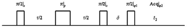
RF pulse sequence for generating and detecting double quantum coherence used in this work. In the experiments the phases were ϕ₁ = x,y,−x,−y and the acquisition phase ϕ₂ = x,−y,−x,y. The phase cycle can be shown to only select double quantum coherence while suppressing zero and single quantum coherences [23,29].

For the condition ${\omega }_q>\frac{1}{T_2}$, which is experimentally realizable, Sharf et al. proposed an approximate form of the time dependence of the Free Induction Decay (FID) for the DQF signal [23]. The result is given by

$$\mathit{\text{FID}}(\tau ,t)=M_{0}sin({\omega }_q\tau )sin({\omega }_{q}t)exp[-(\tau +t)/T_2]$$ (4)

where M₀ is the magnetization of the spins at thermal equilibrium.

By Fourier transformation of the above expression the DQF spectrum can be derived and the real component of the spectrum is approximately [25]

$$\begin{array}{cc}S(\omega ,\tau )\hfill & =sin({\omega }_q\tau )\hfill \\ \hfill & \times exp(-\tau /T_2)\left[\frac{\omega +{\omega }_q}{\omega +{\omega }_q^2+T_2^{-2}}-\frac{\omega -{\omega }_q}{\omega -{\omega }_q^2+T_2^{-2}}\right]\hfill \end{array}$$ (5)

The peak intensity of the spectrum at ω = 0 is given by

$$I=I_{0}sin({\omega }_q\tau )exp(-\tau /T_2)$$ (6)

In systems having a complex morphology, the ²H DQF spectrum may be described by a distribution of different quadrupolar interactions and the total signal is given by

$$I_{\mathit{\text{total}}}=\sum _i{I}_i$$ (7)

where I_i is given by Eq. (6). Eq. (7) shows that the residual quadrupolar interaction, ω_q, may be determined by plotting the peak intensity, I, of the DQF spectrum as a function of τ. In our experimental studies, we found that fitting Eq. (6) to the data was sufficient, therefore all the experimental data were fitted to Eq. (6). The effects of exchange between various sites in the complex morphology of elastin over the time scale of our measurements will be addressed in the following section.

3. Results and discussion

An example of a DQF spectrum acquired at 37 °C with τ = 3.5 ms is given in Fig. 2. Given the Hamiltonian for the quadrupolar interaction in Eq. (1) and the spin operators for I = 1 species proposed by Vega and Pines [30], a numerical simulation of the DQF spectrum was performed on a distribution of 50 nuclear spins by calculating the evolution of the density matrix ρ̂ under the pulse sequence illustrated in Fig. 1. The parameters for the simulation (i.e. ω_q = 170 Hz and T₂ = 4 ms) were derived by fitting Eq. (6) to the experimental DQF signal as a function of τ (open circles shown in Fig. 4). The simulation result is shown in Fig. 2 as a solid line and good agreement with the experimental spectrum shows that using Eq. (6) as a fit to the experimental data is reasonable. It is worth noting that at T = 25 °C the spectrum has been repeated several times and it has been verified that the experimental data is reproducible.

Fig. 2.

Experimental DQF spectrum from D₂O hydrated elastin at 37 °C with τ set to 3.5 ms and δ set to 15 μs. Superimposed on the spectra is a simulation where ω_q was taken to be 170 Hz, and T₂ was set to 4 ms. In both simulation and experimental spectra, a Gaussian line broadening of 5 Hz was applied.

Fig. 4.

Experimental data highlighting the growth and subsequent decay of the DQF signal of deuterated water in elastin. In these experiments the double quantum evolution time δ was set to 15 μs while τ was varied over the range noted on the horizontal axis. The experimental results shown here were collected with the temperature increasing starting from −15 °C. The solid line is a best fit to the experimental data based in Eq. (6).

To verify that the signal collected is indeed a double quantum signal, another experiment was conducted by incrementing the evolution time, δ, while keeping τ = 2 ms with a frequency offset of 100 Hz. In this off-resonance experiment, it is known that the signal intensity associated with a double quantum coherence will oscillate at twice the offset frequency and is given by the expression

$$I=I_{0}cos(2\Delta {\omega }_0\delta )exp(-\delta /T_{DQ})$$ (8)

where Δω₀ is the off-resonance frequency and T_DQ is the double quantum decay time [24]. In the off-resonance experiment, a single quantum coherence arising from free water experiences no anisotropic motion and would oscillate at the offset frequency of 100 Hz. The experimental data from this off-resonance experiment as a function of δ is shown in Fig. 3 with Eq. (8) fit to the data. It is clear from the good agreement with the experimental results that the signal collected using the DQF pulse sequence is indeed a double quantum signal as it oscillates at 200 Hz (i.e. twice the offset frequency) and that the filter via the phase cycling we have implemented is functioning well.

Fig. 3.

Experimental DQF data from D₂O hydrated elastin at 25 °C with τ set to 2 ms and δ varied. The data show that the DQF signal oscillates at twice the offset frequency, which was set to 100 Hz, indicating that the signal detected is indeed a double quantum coherence. The solid line represents a theoretically fitted curve as described in the text.

The τ dependence of the DQF signal of deuterated water in hydrated elastin was measured on both sets of samples described previously. For the sample prepared by method 1. the DQF signals are shown in Figs. 4 and 5 as a function of τ, for increasing and decreasing temperatures, respectively. It should be noted that the DQF signal presented here was determined by the intensity of each DQF spectrum at ω = ω₀. For data analysis we used 30 Hz Gaussian line broadening. Fig. 6 shows the results from samples prepared by method 2. where the elastin fibers were first immersed in solvents. In Figs. 4–6 the solid lines are the best fit curve using Eq. (6).

Fig. 5.

Experimental data highlighting the growth and subsequent decay of the DQF signal of deuterated water in elastin. In these experiments the double quantum evolution time δ was set to 15 μs while τ was varied over the range noted on the horizontal axis. The experimental results shown here were collected with the temperature decreasing, starting from 37 °C. The solid line is a best fit to the experimental data based in Eq. (6).

Fig. 6.

Experimental data highlighting the growth and subsequent decay of the DQF signal of deuterated water in elastin that was saturated in three different solvents, ● D₂O only, ∇ 0.15 M NaCl, ○ DMSO, □ Ethanol. The solid line is a best fit to the experimental data based in Eq. (6).

The parameters resulting from the fit from Eq. (6), ω_q, T₂ and the intensity, I₀ were obtained by minimizing the chi squared, χ² [31]. The uncertainty of each parameter was estimated by varying the corresponding fitting parameter so that the chi-square function increased by 1 [32]. Figs. 7–9 illustrate the results of ω_q, T₂ and I₀ as a function of temperature determined by the best fit, and the error bars for ω_q and I₀ are also plotted in Figs. 7 and 9 respectively. It should be noted that the error bars for T₂ are less than 1% and have been omitted in Fig. 8 for clarity. In addition, the best fit parameters determined from the experimental data in Fig. 6 are given in Table 1.

Fig. 7.

Variation of the residual quadrupolar interaction, ω_q, with temperature determined by fitting Eq. (6) to the experimental data shown in Figs. 5 and 6. The graph shows the changes observed experimentally when the sample was heated from −15 °C to 37 °C and then subsequently cooled from 37 °C to −15 °C The dashed lines are intended to guide the eye and do not represent or intend to be a fit to the data.

Fig. 9.

Variation of the DQF signal intensity with temperature determined by fitting Eq. (6) to the experimental data shown in Figs. 5 and 6. The graph shows the changes observed experimentally when the sample was heated from −15 °C to 37 °C and then subsequently cooled from 37 °C to −15 °C. The dashed lines are intended to guide the eye and do not represent or intend to be a fit to the data.

Fig. 8.

Variation of the T₂ with temperature determined by fitting Eq. (6) to the experimental data shown in Figs. 5 and 6. The graph shows the changes observed experimentally when the sample was heated from −15 °C to 37 °C and then subsequently cooled from 37 °C to −15 °C. The error bars are within 1% and are omitted for clarity. The dashed line is intended to guide the eye and does not represent or intend to be a fit to the data.

Table 1.

Residual quadrupolar interaction, ω_q, and T₂ of D₂O in hydrated elastin in various solvents. The values shown are determined by fitting the experimental data in Fig. 6 to Eq. (6).

Solvents	ωq [Hz]	T2 [ms]
Ethanol	25.3 ± 0.4	5.66 ± 0.05
DMSO	53.6 ± 0.8	5.74 ± 0.06
0.15 M NaCl	40.8 ± 0.5	4.85 ± 0.04
D2O only	92.9 ± 1.7	3.45 ± 0.04

It is clear from Fig. 7 that the residual quadrupolar interaction, ω_q, obeys two different trends when the samples were either heated or cooled. Upon cooling the sample from 37 °C to −15 °C, ω_q increases linearly from 100 Hz to 200 Hz. However, by heating the sample from −15 °C to 37 °C ω_q first reduces from 200 Hz to 150 Hz, then increases to 200 Hz at T = 10 °C and then reduces to 170 Hz as the temperature is further increased. In Fig. 8 the T₂ data shows a scattered pattern for both cases, and is reminiscent of the results published in the similar temperature regime and type of elastin [33]. Fig. 9 shows that the intensity of the DQF signal decreases upon cooling. While with heating the sample from −15 °C the intensity increases slightly but decreases at about T = 10°C and subsequently continues increasing as temperature is further raised. The magnitude of ω_q of water in hydrated bovine nuchal ligament elastin is determined to be between 100 and 200 Hz, and this appears to be close to that observed in collagen fibers [23].

Before further discussing these results, it is instructive that we estimate the spatial dimension over which the anisotropy of the elastin/water system has been studied. The timescale of our DQF experiments range from τ = 0.1 ms up to 30 ms. The time dependent diffusion coefficients of water in elastin have been previously published by our group and are approximately D = 0.9 × 10⁻⁶ (5 °C) to 2.3 × 10⁻⁶ (37 °C) cm²/s over a time scale of 30 ms [34], The root mean square of the spatial displacement is given by

$$\Delta r_{\mathit{\text{rms}}}=\sqrt{6Dt}$$ (9)

Thus, the spatial dimensions we probe via our DQF experiments involve a tortuous 0.2–7 μm of displacement. The spatial dimensions of the elastin fibers are approximately 10 μm in diameter [35] so our measurements likely preclude exchange with water outside a given fiber.

One factor that affects the dynamics of the water molecules and hence the DQF signal is the correlation time, τ_c, of the diffusive motion of water. Although the absolute value of τ_c cannot be measured in our DQF experiment the relative change in τ_c between −15 °C and 37 °C may be estimated by the T₁ data of hydrated bovine nuchal ligament elastin that has been published by Ellis and Packer over a similar temperature range and sample [33]. In their work, two sets of T₁ data were plotted ranging from 0 °C to 70 °C for deuterium in D₂O hydrated elastin. In this high temperature regime the correlation rate, ${\tau }_c^{-1}$, may be described by Arrhenius Law which is given by

$${\tau }_c^{-1}={\tau }_0^{-1}exp(-E_{\mathit{\text{act}}}/k_{B}T)$$ (10)

In the above expression ${\mathit{\tau }}_0^{-1}$ is a constant and E_act is the activation energy of water molecules which is the minimum energy for the molecule to overcome the potential barrier as it tumbles. The spin–lattice relaxation time, T₁, is given by

$$T_1^{-1}=C[f({\omega }_0,{\tau }_c)+4f(2{\omega }_0,{\tau }_c)]$$ (11)

where the spectral density f(ω₀, τ_c) may be expressed by a Lorentzian distribution which is given by

$$f({\omega }_0,{\tau }_c)=C\left[\frac{{\tau }_c}{1+{({\tau }_c{\omega }_0)}^2}\right]$$ (12)

In the above expressions C is a constant that depends on the geometry and is determined by the quadrupolar interaction strength and asymmetry parameter. Generally, at high temperature, the dynamics of the system is in its fast-motion regime where

$${\tau }_c^{-1}\gg {\omega }_0$$ (13)

In this regime Eq. (11) reduces to

$$T_1^{-1}=C{\tau }_c$$ (14)

so

$$T_1={(C{\tau }_c)}^{-1}\propto e^{-E_{\mathit{\text{act}}}/k_{B}T}$$ (15)

Examining the T₁ data for the water with confined motion reported in [33], the activation energy of D₂O in hydrated elastin is estimated to be E_act/k_B = 900K. Using this value for E_act, the relative change in correlation time between −15 °C and 37 °C may be estimated by Eq. (10)

$$\frac{{\tau }_c(37°\text{C})}{{\tau }_c(-15°\text{C})}=\frac{exp(900\text{K}/210\text{K})}{exp(900\text{K}/158\text{K})}=0.25$$ (16)

It should be noted that the above T₁ data published in Ref. [33] allow for only semi-quantitative analysis and therefore the ratio of the correlation times and estimated activation energy is only approximate. The value of the activation energy obtained, is approximately 1/3 of free water and reasonable. The significance of this result is that the dynamics of the waters of hydration, as estimated by T₁ data, changes by a factor of 4 over the range of temperatures indicated. It should also be pointed out that the T₁ data reported in Ref. [33] showed two components, one that was attributed to free water and a second component that had a much longer correlation time. In addition, in their experiments at least three components were observed in the T₂ data. Because the time over which the T₁ experiment is performed is much longer than that of a T₂ experiment, the authors argued that there is significant exchange between the most confined waters of hydration and those having more ‘bulk’ like properties. Thus, the computation above represents an upper bound to the increase in correlation times over the range of temperatures studied.

Fig. 7 shows a monotonic change in ω_q upon cooling the sample, and that the highly confined waters of hydration are more ordered in low temperature than at higher temperatures. This is a manifestation of the decrease in entropy of the water with cooling. At any given temperature, the entropy of water molecules depends on its correlation time and the anisotropy of the tortuous channel to which it is bound. The relative change in ω_q from 37 °C to −15 °C is determined to be approximately 50%, whereas the increase in correlation time is estimated to be 75% from Eq. (16). The 25% discrepancy may be accounted for by the change in anisotropy of the sample upon cooling. Elastin is known to have a negative thermal expansion coefficient resulting from the hydrophobic collapse of the protein [8]. A reduction in temperature results in a macroscopic expansion of the sample and hence gives rise to a less anisotropic environment. Therefore this may effectively offset the increasing change in ω_q by approximately 25%.

Fig. 9 shows that DQF signal intensity is observed to decrease as the temperature was decreased. The physics of this result is that the number of water molecules that experience anisotropic motion is reduced. It appears as if more water molecules are ‘free’; this is consistent with the fact that elastin expands upon cooling because elastin has a negative thermal expansion coefficient so that water molecules have more space to maneuver. Quantitatively, the decrease in the intensity is determined to be 90% from 37 °C to −15 °C. This is consistent with the volume change of hydrated elastin over the same temperature range, estimated by extrapolating to −15 °C whereby the change in volume is estimated to be approximately 80% [8]. It is worth noting that over the same temperature range, the change in ω_q arising from the change in elastin's volume is only 25% as discussed above. This may show that although the anisotropic motion of water molecules is correlated to the overall volume changes of elastin, the percentage changes are different and may point to a more complex exchange between various compartments.

Fig. 8 shows that the T₂ data is scattered with temperature and no clear trends can be drawn. This may be due to the fact that T₂ is very sensitive to intrinsic parameters such as field inhomogeneity and sample susceptibility that may change as the sample temperature is varied. Nevertheless, the variation of the T₂ data is in good agreement with the data published by Ellis and Packer [33]. As mentioned previously, in their work, three T₂ components were measured where the longest and shortest values were assigned to the bulk and bound waters respectively. The intermediate component was interpreted as the exchange between the former two. In our work, only one component is revealed by the DQF experiment as this experiment only detects the most bound water molecules experiencing anisotropic motion. The value of the T₂ measured via the DQF experiments is in good agreement with the shortest value measured in Ref. [33].

Unlike the data measured upon cooling, Figs. 7 and 9 reveal that by heating the sample there is a substantial increase both in ω_q and decrease in DQF signal intensity at about T = 10 °C to T = 15 °C. We attribute these marked changes to the hydrophobic collapse of the protein. The observation that the DQF intensity decreases near this transition temperature corroberates other studies. It has also been observed that the overall number of highly confined water molecules are reduced upon heating the sample as the protein pushes water out of the complex morphology that gives rise to its elasticity [10,12]. At the inverse temperature transition, it has been shown that elastin's length may be reduced by as much as 15% per 10 °C, determined by temperature dependent stress–strain studies [9]. In our experimental work, we observe ω_q increases from 5 °C to 15 °C by approximately 35%. As ω_q is a sensitive measure of local anisotropy and elastin shrinks upon heating, it is expected that residual quadrupolar interaction be related to the macroscopic volumetric changes of the biopolymer. The small difference may arise from the conformational change of elastin involving three dimensions, whereas only a change in length was considered in the aforementioned study. Further, in our work, the inverse temperature transition occurs near 10–15 °C. However, in polypentapeptide studies the transition was observed to occur in a range of 20–40 °C [9], and more directly in the simulation studies of (VPGVG)₁₈ it was predicted to occur in the range of 20–30 °C [13]. The shift in the transition temperature T_t may be accounted for by the fact that the inverse temperature transition can be changed by changing the hydrophobicity of a given polypeptide [10]. Moreover, the hydrophobicity can be affected by changing the amino-acid sequence [14]. For example, the transition temperature can be shifted from 30 °C to 10 °C by increasing the hydrophobicity of a given peptide [10]. Therefore the hydrophobicity of the nuchal ligament elastin studied in our work may be greater than that which was simulated in the polypentapeptide studies in Ref. [13]. It should be pointed out that we also observe a subsequent decrease in ω_q above 15 °C, as the temperature is further increased. We believe that this may be due to the increase in thermally driven motion of the water molecules as the temperature is raised above T = 15 °C.

The change in the DQF signal intensity in our experimental data from 5 °C to 15 °C also supports the notion of an inverse temperature transition phenomenon. As the DQF intensity is a manifestation of the number of hydrated water molecules that experience a residual quadrupolar interaction, our results point to the intensity decreasing by 70% over this temperature range, whereas in simulation studies from 20 °C to 30 °C the number of hydrated water molecules is decreased by only 8% [13]. While the trends are in agreement in simulation and experiment, the difference may arise from two effects. First, as discussed above, the hydrophobicity of our sample may be greater than the elastin-like peptide model that was simulated, and therefore a more dramatic hydrophobic effect may be observed. Second, the timescale over which our experiment was performed was over a range of ms while the simulations were performed over several ns. The longer time scale probed in the experiment may incorporate a complex water–protein interaction as well as exchange between various domains in the complex morphology not realized in the simple simulation. We also observe that upon increasing the temperature above 15 °C that there is a subsequent increase in the DQF signal intensity, and we attribute this change to the negative thermal expansion of the sample.

It is well known that immersing elastin in polar solvents may change the system hydrophobicity and hence the dynamics of water that are confined to it. In our work, the DQF signal of elastin in three solvents was studied and the best fit for ω_q and T₂ are tabulated in Table 1. Before discussing our results it is worth reviewing the ¹³C NMR studies on hydrated elastin in solvents studied via conventional liquid state NMR methods [7]. In their work, without any solvents, the carbonyl, α-backbone and methyl carbons are evident in the spectra. Once the solvents are introduced, the spectra are changed differently. For ethanol (dielectric constant ε = 24), the carbonyl carbon peak disappears and this shows that the mobility at this site is reduced in this solvent. With DMSO (ε = 45) the phenyl carbon peak is easily observed, and this reveals that the solvent induces the phenyl group to be more mobile. For 0.15 M NaCl (ε ∼ 70 for NaCl in water) the α-backbone carbon peak is broadened showing a reduction in the global mobility of the protein. It is clear from their spectra that the solvents change the mobility of elastin and the introduction of different solvents induces the mobility of various sites. Table 1 shows that the residual quadrupolar interaction is decreased and that T₂ increases for the three samples with different solvents compared with the sample prepared by method 1. This shows that in the solvents studied, the highly confined hydrated water molecules become more mobile compared to a sample that is merely hydrated in water. Lastly, the trend in the observed reduction in ω_q with decreasing dielectric constant also points to a reduction in the overall anisotropy of the motion of water in elastin.

4. Conclusion

In this work we have investigated the dynamics of water in deuterium hydrated bovine nuchal ligament elastin. Our results indicate that there is an increase in order in the surrounding waters of hydration in elastin upon increasing the temperature near 10–15°C. The studies support an already existing notion of hydrophobic collapse near this temperature. We studied the change in the residual quadrupolar interaction at 37 °C, and observed that there is a strong correlation to the dielectric constant of the solvent. While our work probed the dynamics over a time scale of 0.1–30 ms it is not clear to what extent chemical exchange occurs between various compartments in the complex morphology of this biopolymer and is the subject of future work in our laboratory.

References

- 1.Lillie MA, Gosline JM. The effects of polar solutes on the viscoelastic behavoir of elastin. Biorheology. 1993;30:229–242. doi: 10.3233/bir-1993-303-408. [DOI] [PubMed] [Google Scholar]
- 2.Hoeve CAJ, Flory PJ. The elastic properties of elastin. J Am Chem Soc. 1958;80:6523–6526. [Google Scholar]
- 3.Hoeve CAJ, Flory PJ. The elastic properties of elastin. Biopolymers. 1974;23:677–686. doi: 10.1002/bip.1974.360130404. [DOI] [PubMed] [Google Scholar]
- 4.Gray WR, Sandberg LB, Foster JA. Molecular model for elastin structure and function. Nature. 1973;246:461–466. doi: 10.1038/246461a0. [DOI] [PubMed] [Google Scholar]
- 5.Dorrington K, Grut W, McCrum NG. Mechanical state of elastin. Nature. 1975;255:476–478. [Google Scholar]
- 6.Weis-Fogh T, Andersen SO. New molecular model for the long-range elasticity of elastin. Nature. 1970;227:718–721. doi: 10.1038/227718a0. [DOI] [PubMed] [Google Scholar]
- 7.Lyerla JR, Jr, Torchia DA. Molecular mobility and structure of elastin deduced from the solvent and temperature dependence of 13C magnetic resonance relaxation data. Biochemistry. 1975;14:5175–5183. doi: 10.1021/bi00694a024. [DOI] [PubMed] [Google Scholar]
- 8.Mistrali F, Volpin D, Garibaldo GB, Ciferri A. Thermodynamics of elasticity in open systems: elastin. J Phys Chem. 1971;75:142–150. doi: 10.1021/j100671a023. [DOI] [PubMed] [Google Scholar]
- 9.Urry DW, Haynes B, Harris RD. Temperature dependence of length of elastin and its polypentapeptide. Biochem Biophys Res Commun. 1986;141:749–755. doi: 10.1016/s0006-291x(86)80236-4. [DOI] [PubMed] [Google Scholar]
- 10.Urry DW. Entropic elastic processes in protein mechanisms. I. Elastic structure due to an inverse temperature transition and elasticity due to internal chain dynamics. J Protein Chem. 1988;7:1–34. doi: 10.1007/BF01025411. [DOI] [PubMed] [Google Scholar]
- 11.Luan CH, Parker TM, Prasad KU, Urry DW. Differential scanning calorimetry studies of NaCl effect on the inverse temperature transition of some elastin-based polytetra-, polypenta-, and polynonapeptides. Biopolymers. 1991;31:465–475. doi: 10.1002/bip.360310502. [DOI] [PubMed] [Google Scholar]
- 12.Reierson H, Clarke AR, Rees AR. Short elastin-like peptides exhibit the same temperature-induced structural transitions as elastin polymers: implications for protein engineering. J Mol Biol. 1998;283:255–264. doi: 10.1006/jmbi.1998.2067. [DOI] [PubMed] [Google Scholar]
- 13.Li B, Alonso DOV, Daggett V. The molecular basis for the inverse temperature transition of elastin. J Mol Biol. 2001;305:581–592. doi: 10.1006/jmbi.2000.4306. [DOI] [PubMed] [Google Scholar]
- 14.Ribeiro A, Arias FJ, Reguera J, Alonso M, Rodriguez-Cabello JC. Influence of the amino-acid sequence on the inverse temperature transition of elastin-like polymers. Biophys J. 2009;97:312–320. doi: 10.1016/j.bpj.2009.03.030. [DOI] [PMC free article] [PubMed] [Google Scholar]
- 15.Dill KA, Privalov PL, Gill SJ, Murphy KP. The meaning of hydropobicity. Science. 1990;250:297–298. doi: 10.1126/science.2218535. [DOI] [PubMed] [Google Scholar]
- 16.Urry DW, Trapane TL, Prasad KU. Phase-structure transitions of the elastin polypentapeptide-water system within the framework of composition-temperature studies. Biopolymers. 1985;24:2345–2356. doi: 10.1002/bip.360241212. [DOI] [PubMed] [Google Scholar]
- 17.Urry DW. What is elastin; what is not. Ultrastruct Pathol. 1983;4:227–251. doi: 10.3109/01913128309140793. [DOI] [PubMed] [Google Scholar]
- 18.Urry DW, Long MM. Conformations of the repeat peptides of elastin in solution: an application of proton and carbon-13 magnetic resonance to the determination of polypeptide secondary structure. CRC Crit Rev Biochem. 1976;4:1–45. doi: 10.3109/10409237609102557. [DOI] [PubMed] [Google Scholar]
- 19.Urry DW, Shaw RG, Prasad KU. Polypentapeptide of elastin: temperature dependence of ellipticityand correlation with elastomeric force. Biochem Biophys Res Commun. 1985;130:50–57. doi: 10.1016/0006-291x(85)90380-8. [DOI] [PubMed] [Google Scholar]
- 20.Urry DW, Trapane TL, McMichens RB, Iqbal M, Harris RD, Prasad KU. Nitrogen-15 NMR relaxation study of inverse temperature transitions in elastin polypentapeptide and its crosslinked elastomer. Biopolymers. 1986;25:S209–S228. [PubMed] [Google Scholar]
- 21.Urry DW. Protein elasticity based on conformations of sequential polypeptides: the biological elastic fiber. J Protein Chem. 1984;3:403–436. [Google Scholar]
- 22.Henze R, Urry DW. Dielectric relaxation studies demonstrate a peptide librational mode in the polypentapeptide of elastin. J Am Chem Soc. 1985;107:2991–2993. [Google Scholar]
- 23.Sharf Y, Eliav U, Shinar H, Navon G. Detection of anisotroscopy in cartilage using 2H double-quantum-filtered NMR-spectroscopy. J Magn Reson Ser B. 1995;107:60–767. [Google Scholar]
- 24.Shinar H, Seo Y, Navon G. Discrimination between the different compartments in sciatic nerve by 2H double-quantum-filtered NMR. J Magn Reson. 1997;129:98–104. doi: 10.1006/jmre.1997.1250. [DOI] [PubMed] [Google Scholar]
- 25.Perea W, Cannella M, Yang J, Vega AJ, Polenova T, Marcolongo M. 2H double quantum filtered (DQF) NMR spectroscopy of the nucleus pulposus tissues of the intervertebral disc. Magn Reson Med. 2007;57:990–999. doi: 10.1002/mrm.21231. [DOI] [PubMed] [Google Scholar]
- 26.Navon G, Shinar H, Eliav U, Seo Y. Multiquantum filters and order in tissues. NMR Biomed. 2001;14:112–132. doi: 10.1002/nbm.687. [DOI] [PubMed] [Google Scholar]
- 27.Partridge SM, Davies HF, Adair GS. The chemistry of connective tissues: 2. Soluble proteins derived from partial hydrolysis of elastin. Biochem J. 1955;61:11–21. doi: 10.1042/bj0610011. [DOI] [PMC free article] [PubMed] [Google Scholar]
- 28.Levitt MH. Spin Dynamics: Basics of Nuclear Magnetic Resonance. John Wiley and Sons Ltd.; 2001. pp. 201–202. [Google Scholar]
- 29.Bedenhausen G, Vold RL, Vold RR. Multiple quantum spin-echo spectroscopy. J Magn Reson. 1980;37:93–106. [Google Scholar]
- 30.Vega S, Pines A. Operator formalism for double quantum NMR. J Chem Phys. 1977;66:5624–5644. [Google Scholar]
- 31.Bevington PR, Robinson DK. Data Redcution and Error Analysis for the Physical Sciences. second. Vol. 8. McGraw-Hill, Inc.; 1992. pp. 141–167. [Google Scholar]
- 32.Arndt RA, MacGregor MH. Nucleon–nucleon phase shift analysis by chi-squared minimization. Methods Comput Phys. 1966;6:253–296. [Google Scholar]
- 33.Ellis GE, Packer KJ. Nuclear spin-relaxation studies of hydrated elastin. Biopolymers. 1976;15:813–832. doi: 10.1002/bip.1976.360150502. [DOI] [PubMed] [Google Scholar]
- 34.Boutis G, Renner C, Isahkarov T, Islam T, Kannangara L, Kaur P, Mananga E, Ntekim A, Rumala Y, Wei D. High resolution q-space imaging studies of water in elastin. Biopolymers. 2007;87:352–359. doi: 10.1002/bip.20838. [DOI] [PubMed] [Google Scholar]
- 35.Gotte L, Mammi M, Pezzin G. Scanning electron microscope observation on elastin. Connect Tissue Res. 1972;1:61–67. [Google Scholar]