SPIRiT: Iterative Self-consistent Parallel Imaging Reconstruction from Arbitrary k-Space

Abstract

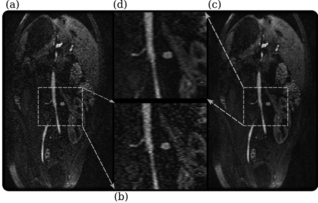
A new approach to autocalibrating, coil-by-coil parallel imaging reconstruction is presented. It is a generalized reconstruction framework based on self consistency. The reconstruction problem is formulated as an optimization that yields the most consistent solution with the calibration and acquisition data. The approach is general and can accurately reconstruct images from arbitrary k-space sampling patterns. The formulation can flexibly incorporate additional image priors such as off-resonance correction and regularization terms that appear in compressed sensing. Several iterative strategies to solve the posed reconstruction problem in both image and k-space domain are presented. These are based on a projection over convex sets (POCS) and a conjugate gradient (CG) algorithms. Phantom and in-vivo studies demonstrate efficient reconstructions from undersampled Cartesian and spiral trajectories. Reconstructions that include off-resonance correction and nonlinear ℓ₁-wavelet regularization are also demonstrated.

Introduction

Multiple receiver coils have been used since the beginning of MRI (1), mostly for the benefit of increased signal to noise ratio (SNR). In the late 80’s, Kelton, Magin and Wright proposed in an abstract (2) to use multiple receivers for scan acceleration. However, it was not until the late 90’s when Sodickson et al. presented their method SMASH (3) and later Pruessmann et al. presented SENSE (4), that accelerated scans using multiple receivers became a practical and viable option.

Multiple receiver coil scans can be accelerated because the data obtained for each coil are acquired in parallel and each coil image is weighted differently by the spatial sensitivity of its coil. This sensitivity information in conjunction with gradient encoding reduces the required number of data samples that is needed for reconstruction. This concept of reduced data acquisition by combined sensitivity and gradient encoding is widely known as parallel imaging.

Over the years, a variety of methods for parallel imaging reconstruction have been developed. These methods differ by the way the sensitivity information is used. Methods like SMASH (3), SENSE (4,5), SPACE-RIP (6), PARS (7) and kSPA (8) explicitly require the coil sensitivities to be known. In practice, it is very difficult to measure the coil sensitivities with high accuracy. Errors in the sensitivity are often amplified and even small errors can result in visible artifacts in the image (9). On the other hand, autocalibrating methods like AUTO-SMASH (10, 11), PILS (12), GRAPPA (13) and APPEAR (14) implicitly use the sensitivity information for reconstruction and avoid some of the difficulties associated with explicit estimation of the sensitivities. Another major difference is in the reconstruction target. SMASH, SENSE, SPACE-RIP, kSPA and AUTO-SMASH attempt to directly reconstruct a single combined image. Coil-by-coil methods, PILS, PARS and GRAPPA directly reconstruct the individual coil images leaving the choice of combination to the user. In practice, coil-by-coil methods tend to be more robust to inaccuracies in the sensitivity estimation and often exhibit fewer visible artifacts (9, 14, 15).

SENSE is an explicit sensitivity-based, single image reconstruction method. Among all methods, the SENSE approach is the most general. It provides a framework for reconstruction from arbitrary k-space sampling and to easily incorporate additional image priors. When the sensitivities are known, SENSE is the optimal solution (14, 15). To the best of the authors’ knowledge, none of the coil-by-coil autocalibrating methods are as flexible and optimal as SENSE. Some proposed methods (16–19) adapt GRAPPA to reconstruct some non-Cartesian trajectories, but these require approximations and therefore lose some of the ability to remove all the aliasing artifacts.

Here, we propose a new approach to parallel imaging reconstruction called SPIRiT. It is a coil-by-coil autocalibrating reconstruction. It is heavily based on the GRAPPA reconstruction, but also draws its inspiration from SENSE in the sense that the reconstruction is formulated as an inverse problem in a very general way. The end result is that the reconstruction is the solution for a least-squares optimization. SPIRiT is based on self-consistency with the calibration and acquisition data. It is flexible and can reconstruct data from arbitrary k-space sampling patterns and easily incorporates additional image priors. SPIRiT stands for iTerative Self-consistent Parallel Imaging Reconstruction.

In this paper we first review the foundations of SPIRiT, e.g., the GRAPPA method. We then define the SPIRiT consistency constraints and show that the reconstruction is a solution to an optimization problem. We then extend the method to arbitrary sampling patterns with k-space-based and image-based approaches. Finally we show that the method can easily introduce additional priors such as off-resonance correction and regularization.

Cartesian GRAPPA

The GRAPPA reconstruction poses the parallel imaging reconstruction as a translation variant interpolation problem in k-space. It is a self-calibrating coil-by-coil reconstruction method. Unlike SENSE, which attempts to reconstruct a single combined image, GRAPPA attempts to reconstruct the individual coil images directly.

In the traditional GRAPPA (13) algorithm a non-acquired k-space value in the i^th coil, at position r, x_i(r), is synthesized by a linear combination of acquired neighboring k-space data from all coils. Let R_r be a set of operators that choose points from a single-coil Cartesian k-space, such that the product R_rx_i is a vector containing the k-space points in the neighborhood of position r. Let R͂_r be the operators that choses a smaller subset of only the acquired k-space locations in the neighborhood of position r. The recovery of x_i(r) is given by:

$$x_i(r)={\displaystyle \sum _j{g}_{rji}^{*}({\tilde{R}}_r{x}_i),}$$ (1)

where g_rji is a vector set of weights obtained by calibration for the particular sampling pattern around position r, and $g_{rji}^{*}$ is its transpose-conjugate. The full k-space grid is reconstructed by solving [Eq. 1] for each un-acquired k-space in all coils and all positions.

The linear combination weights, or calibration kernel, used in [Eq. 1] are obtained by calibration from a fully acquired k-space region. The calibration finds the set of weights that is the most consistent with the calibration data in the least-squares sense. In other words, the calibration stage looks for a set of weights such that if one tries to synthesize each of the calibration points from their neighborhood the result should be as close as possible to the true calibration points. More formally, the calibration is described by the following equation:

$$arg\underset{{\mathbf{g}}_{\mathbf{r}\mathbf{i}}}{\text{min}}{\displaystyle \sum _{\rho \epsilon \text{Calib}}{\Vert {\displaystyle \sum _j{g}_{rji}^{*}({\tilde{R}}_{\rho }{x}_j)-x_i(\rho )}\Vert }^2,}$$ (2)

where g_ri is a concatenation of all g_rji’s or, g_ri = [g_{r 1i}, …g_{r 2i}, …,g_rNi]^T. The above can be written in matrix form as:

$$arg\underset{{\mathbf{g}}_{\mathbf{r}\mathbf{i}}}{\text{min}}{\Vert \tilde{X}*g_{ri}-x_i\Vert }^2,$$ (3)

in which the entries of X͂ are all the R͂_rx_i vectors in the calibration area of k-space that were reordered into a matrix. This equation is often solved as Tykhonov regularized least-squares which has the analytic solution:

$$g_{ri}={(\tilde{X}*\tilde{X}+\beta I)}^{-1}\tilde{X}*x_i.$$ (4)

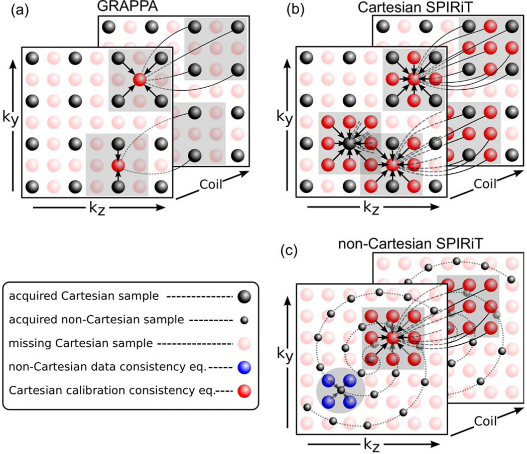
The assumption is that if the calibration consistency holds within the calibration area, it also holds in other parts of k-space. Therefore [Eq. 1] can be used for the reconstruction. In the original GRAPPA paper, the undersampling pattern was such that the k-space sampling in the neighborhood of the missing points is the same for all points. Therefore a single set of weights is enough for reconstruction and the calibration can be performed only once. In 2D acceleration however, the sampling pattern around each missing point can be quite different. Different sets of weights must be obtained for each sampling pattern. As an illustration, consider the 2D GRAPPA reconstruction in Fig. 1a. The figure portrays two equations to solve two missing data points. Each of the equations uses a different set of calibration weights. The neighborhood size in that example for illustration purposes is a square of three k-space pixels.

Figure 1.

(a) Traditional 2D GRAPPA: Missing k-space data are synthesized from neighboring acquired data. The synthesizing kernel depends on the specific sampling pattern in the neighborhood of the missing point. The reconstruction of a point is independent of the reconstruction of other missing points. (b) Cartesian SPIRiT reconstruction: Three consistency equations are illustrated. The reconstruction of each point on the grid is dependent on its entire neighborhood. The reconstruction of missing points depends on the reconstruction of other missing points. The calibration consistency equation is independent of the sampling pattern. (c) Non-Cartesian SPIRiT: The calibration consistency equation is Cartesian (red). The acquisition data consistency relation between the Cartesian missing points and the non-Cartesian acquired points is shown in blue. These define a large set of linear equations that is sufficient for reconstruction.

Methods

SPIRiT: a Self Consistency Formulation

Inspired by GRAPPA, we take on a slightly different approach that has similar properties to GRAPPA, but is more general and uses the data more efficiently. Our aim is to describe the reconstruction as an inverse problem governed by data consistency constraints. The key in the approach is to separate the consistency constraints into a) consistency with the calibration, and b) consistency with the data acquisition. We formulate these constraints as sets of linear equations. The desired reconstruction is the solution that satisfies the sets of equations best according to a suitable error measure criteria.

Even though the acquired k-space data may or may not be Cartesian, ultimately, the desired reconstruction is a complete Cartesian k-space grid for each of the coils. Therefore, we define the entire Cartesian k-space grid for all the coils as the unknown variables in the equations. This step makes the formulation very general especially when considering noisy data, regularization and non-Cartesian sampling.

Consistency with the Calibration

Traditional GRAPPA enforces calibration consistency only between synthesized points and the acquired points in their associated neighborhoods. The proposed approach expands the notion of consistency by enforcing consistency between every point on the grid, x_i(r), and its entire neighborhood across all coils (e.g., R_rx_j). It is important to emphasize that the notion, entire neighborhood, includes all the k-space points near x_i(r) in all coils whether they were acquired or not. Given the above, the consistency equation for all k-space positions is given by,

$$x_i(r)={\displaystyle \sum _j{g}_{ji}^{*}(R_r{x}_j).}$$ (5)

The difference between g_ji here and the traditional GRAPPA weights g_rji in [Eq. 1], is that g_ji is a full kernel independent of the actual k-space sampling pattern and is the same for all k-space positions. It is obtained by using the operators R_r instead of R͂_r in [Eq. 2]. [Equation 1] defines a large set of decoupled linear equations that can be solved separately. On the other hand, [Eq. 5] defines a large set of coupled linear equations. As an illustration, consider Fig. 1b which has a similar sampling setup as the 2D GRAPPA problem in Fig. 1a. In the figure, three equations are portrayed. It shows that the synthesis of a missing central point depends on both acquired and missing points in its neighborhood and that the equations are coupled.

It is convenient to write the entire coupled system of equations in matrix form. Let x be the entire k-space grid data for all coils, and let G be a matrix containing the g_ji’s in the appropriate locations. The system of equations can simply be written as,

$$x=Gx.$$ (6)

The matrix G is in fact a series of convolution operators (denoted as a ⊗ b) that convolve the entire k-space with the appropriate calibration kernels,

$$x_i={\displaystyle \sum _j{g}_{ij}\otimes x_j.}$$ (7)

[Equations 6–7] can be explained intuitively. Applying the operation G on x is the same as attempting to synthesize every point from its neighborhood. If x is indeed the correct solution then synthesizing every point from its neighborhood should yield the exact same k-space data!

Consistency with the Data Acquisition

Of course, any plausible reconstruction has to be consistent with the real data that were acquired by the scanner. This constraint can also be expressed as a set of linear equations in matrix form. Let y be the vector of acquired data from all coils (concatenated). Let the operator D be a linear operator that relates the reconstructed Cartesian k-space, x, to the acquired data. The data acquisition consistency is given by

$$y=Dx.$$ (8)

This formulation is very general in the sense that x is always Cartesian k-space data, whereas y can be data acquired with arbitrary k-space sampling patterns. In Cartesian acquisitions, the operator D selects only acquired k-space locations. The selection can be arbitrary: uniform, variable density or pseudo random patterns. In non-Cartesian sampling, the operator D represents an interpolation matrix. It interpolates data from a Cartesian k-space grid onto non-Cartesian k-space locations in which the data were acquired.

Constrained Optimization Formulation

[Equations 6] and [8] describe the calibration and data acquisition consistency constraints as sets of linear equations that the reconstruction must satisfy. However, due to noise and calibration errors these equations can only be solved approximately. Therefore, we propose as reconstruction the solution to an optimization problem given by,

$$\begin{array}{ll}\text{minimize}\hfill & {\Vert (G-I)x\Vert }^2\hfill \\ \mathrm{s}.\mathrm{t}.\hfill & {\Vert Dx-y\Vert }^2\le \epsilon .\hfill \end{array}$$ (9)

The parameter ε is introduced as a way to control the consistency. It trades off data acquisition consistency with calibration consistency. The beauty in this formulation is that the calibration consistency is always applied to a Cartesian k-space, even though the acquired data may be non-Cartesian. The treatment of non-Cartesian sampling appears only in the data acquisition constraint. This is illustrated more clearly in Fig. 1c.

A useful reformulation of [Eq. 9] is the unconstrained Lagrangian form,

$$arg\underset{\mathbf{x}}{\text{min}}{\Vert Dx-y\Vert }^2+\lambda (\epsilon ){\Vert (G-I)x\Vert }^2.$$ (10)

As is well known, the parameter λ can be chosen appropriately such that the solution of [Eq. 10] is exactly as [Eq. 9]. In general the optimization in [Eq. 9–Eq. 10] and variations of it can often be solved very efficiently by iterative descent methods such as steepest descent or the much more efficient conjugate gradient algorithm. These are all based on the ability to rapidly calculate the gradient of the objective function which is,

$${\nabla }_x\{{\Vert Dx-y\Vert }^2+\lambda {\Vert (G-I)x\Vert }^2\}=2D*(Dx-y)+\lambda 2(G-I)*(G-I)x.$$ (11)

A steepest descent algorithm with a step-size μ would simply calculate

$$x_{n+1}=x_n-\mu [D*(D-y)+\lambda (G-I)*(G-I)x],$$

at every iteration. It is fortunate that in the cases discussed in this paper, both the G and D operation and their adjoints G* and D* can be calculated very quickly. In the next sections we will provide the reconstruction details for more specific examples, including the calculation of the G and D operators and their adjoints.

Arbitrary Cartesian Sampling

In some cases it may be useful to leave the acquired k-space unchanged. This is equivalent to enforcing data acquisition equality constraint (i.e., ε → 0 in [Eq. 9]). One way to implement this is through continuation by starting with a large value of λ and then iteratively reducing it while repeatedly solving [Eq. 10]. A simpler and more efficient approach is to incorporate the equality constraint in the objective, such that the problem is formulated as simple least-squares. Let y be the vector of acquired points, let x͂ now be the vector representing only the missing points, let D and D_c be the matrices that select the acquired and non-acquired points out of the full k-space grid respectively. This way, D^T and $D_c^T$ take the selected acquired and non-acquired samples and put them back in the right location in the full k-space grid. We can now write x as, $x=D^{T}y+D_c^T\tilde{x}$ Substituting into [Eq. 9] we get,

$$\begin{array}{ll}arg\underset{\tilde{\mathbf{x}}}{\text{min}}\hfill & {\Vert Dx-y\Vert }^2+\lambda {\Vert (G-I)x\Vert }^2\hfill \\ =arg\underset{\tilde{\mathbf{x}}}{\text{min}}\hfill & {\Vert D(D^{T}y+D_c^T\tilde{x})-y\Vert }^2+\lambda {\Vert (G-I)(D^{T}y+D_c^T\tilde{x})\Vert }^2\hfill \\ =arg\underset{\tilde{\mathbf{x}}}{\text{min}}\hfill & {\Vert y+0-y\Vert }^2+\lambda {\Vert (G-I)D_c^T\tilde{x}+(G-I)D^{T}y\Vert }^2\hfill \\ =arg\underset{\tilde{\mathbf{x}}}{\text{min}}\hfill & {\Vert (G-I)D_c^T\tilde{x}+(G-I)D^{T}y\Vert }^2,\hfill \end{array}$$ (12)

which has the usual format of a least-norm-least-squares problem, e.g., argmin_x ∥Ax – b∥, where $A=(G-I)D_c^T$ and b = –(G – I)D^Ty. This can be solved directly using sparse matrices or iteratively using standard descent algorithms like conjugate gradient. Another efficient alternative is to find a solution for Gx = x using a projection over convex sets (POCS) algorithm. The POCS approach is described in Table 1.

Table 1.

A POCS algorithm for SPIRiT from arbitrary sampling on a Cartesian grid.

	POCS SPIRiT CARTESIAN RECONSTRUCTION
INPUTS:
	y - k-space measurements from all coils
	D - operator selecting acquired k-space
	Dc - operator selecting non-acquired k-space
	G - SPIRiT operator matrix obtained from calibration
	errToll - stopping tolerance
OUTPUTS:
	xk - reconstructed k-space for all coils
ALGORITHM:
	x0 = DT y; k = 0
	do {
	k = k+1
	xk = Gxk–1 % Calibration consistency projection
	$x_k=D_c^T{D}_c{x}_k+D^{T}y\%$Dcxk + DT y % Data acquisition consistency projection
	e = ∥xk - xk–1∥ % Error stopping criteria
	xk–1=xk
	}while e > errToll

Non-Cartesian Sampling

In theory, [Eq. 9] is the solution for the non-Cartesian case. However, the practical success of the reconstruction depends on how well the operators G and D approximate the true data, and how fast they can be computed in practice. The main difficulty facing the reconstruction is an accurate and efficient interpolation scheme in k-space. Next, we present two approaches. The first operates entirely in k-space. The other also applies calculations in the image domain.

Calibration

The SPIRiT approach is autocalibrating. We assume that there is always a subset of k-space that is sufficiently sampled for the purpose of calibration. For example, radial trajectories and dual density spiral (18) trajectories have a region around the k-space origin that is sufficiently sampled. From such data, Cartesian calibration data are obtained by interpolation. Alternatively, such a Cartesian calibration region can be obtained by a separate scan. The full kernel weights are calculated from calibration data similar to [Eq. 4].

A) k-Space Domain Reconstruction

The most natural way to approximate the data consistency constraint y = Dx is to use convolution interpolation to interpolate from Cartesian onto the non-Cartesian k-space grid and vice versa. This is very similar to the gridding algorithm. However, several details need to be taken into consideration.

Consider a convolution interpolation of the i ^th coil’s k-space data from a Cartesian grid to a non-Cartesian grid. Let c be an interpolation kernel, k be the non-Cartesian k-space coordinates, and δ(x) the usual impulse function. One can write the operation D applied to the i ^th coil’s data as,

$$y_i(n)={\displaystyle {\int }_r\delta (k(n)-r)\{c*x_i\}(r)dr}$$ (13)

Ideally, the interpolation kernel, c, should be a sinc function. However, this has a prohibitively large kernel size. Traditionally, in the gridding algorithm (20), a very small kernel is used to reduce the computation. The errors associated with a small kernel are mitigated by oversampling the grid, and the associated image weighting is mitigated by a deapodization of the resulting image to correct the intensity weighting. The gridding algorithm in effect trades off complexity with tolerable accuracy errors. In the proposed reconstruction, the data acquisition consistency in [Eq. 8] is enforced. Therefore, the consistent solution when using a non-sinc kernel can not be exactly x͂_i, but a function of it, x_i. Let c͂ be a convolution kernel such that c*c͂ = δ. then

$${\tilde{x}}_i=\tilde{c}*x_i,$$ (14)

so, c*x _{i͂ = c * c͂ * xi} ≈ x_i.

In the image domain this function is manifested as a multiplication by a deapodizing function

$$\begin{array}{ll}{\tilde{m}}_i(r)\hfill & =\tilde{C}(r)m_i(r)\hfill \\ \hfill & =\frac{1}{C(r)}{m}_i(r),\hfill \end{array}$$ (15)

where m_i, m͂_i, and C denote the inverse Fourier transform of of x_i, C͂ and c respectively.

In the usual gridding reconstruction, such weighting is generally not a problem and is easily compensated. However, in our case, the solution x͂ may no longer be consistent with the data calibration constraint in [Eq. 6]. This is in particular a problem when using a Kaiser-Bessel kernel, which has large variations across the imaged field of view. Any amplitude variation in the field of view will amplify residual aliasing. To mitigate this, one should design a kernel with ripple constraints on the passband as well as the stopband. For example, a windowed-sinc kernel would introduce much less variation than the Kaiser-Bessel kernel would. An optimized alternative is to modify the min-max SOCP interpolator by Beatty (21) to include the image intensity variation constraint.

Revisiting the Calibration

The grid oversampling in k-space requires that the calibration kernel support be increased by the same amount. For example, if normally one would chose to use a 5 × 5 size kernel in a GRAPPA reconstruction, and a grid oversampling is 1.2, then a 6 × 6 size kernel should be used. In addition, the sampling trajectory of the calibration region must be oversampled to support the larger FOV of the oversampled grid, or else the fidelity and integrity of the calibration may be compromised. Finally, the interpolation kernel that grids the calibration region should have as little passband ripple as possible, again to ensure the fidelity of the calibration process.

Reconstruction

The steps for non-Cartesian k-space based reconstruction are as follows:

• Design an appropriate interpolation kernel based on a specific maximum aliasing amplitude, image weighting, kernel width and grid oversampling

• Perform a calibration that supports the oversampled grid size to obtain the calibration weights

• Solve Eq. 10 using the conjugate gradients algorithm to obtain reconstructed Cartesian k-space data for all coils

• Reconstruct the images by computing the inverse Fourier transform

• Crop to the desired grid size

• Apodize the images by multiplying with the inverse Fourier transform of the interpolation kernel.

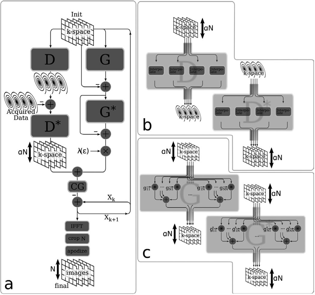
It is important to note that an efficient and numerically stable implementation of the POCS approach for non-Cartesian imaging is challenging for reasons outside the scope of this paper, therefore we prefer the CG approach in this case. A diagram for the conjugate gradient algorithm implementation is described in detail in Fig 2a. The top part, calculates the gradient of the objective function as described by [Eq. 11]. The current estimate of k-space (on the oversampled grid) is split into two paths. The left path computes the gradient of the acquisition data consistency term by interpolating the current estimate onto a non-Cartesian grid. Then, computing the difference error with the acquired data and interpolating that error back onto a Cartesian grid. The right path computes the gradient of the calibration data consistency by performing the SPIRiT convolution, convolving the result with its adjoint, and finally scaling with λ. The calculated gradient is then used to find a conjugate gradient direction which is subtracted from the previous estimate of k-space. After the iterations converge, an inverse FFT is performed for each coil, the images are cropped to the appropriate FOV and apodized by the inverse Fourier transform of the k-space convolution interpolation kernel.

Figure 2.

k-Space based reconstruction. (a) Illustration of the conjugate-gradient algorithm for non-Cartesian consistency constrained reconstruction in k-space. (b) Illustration of the interpolation operator, D, and its adjoint, D* (c) Illustration of the calibration consistency operator, G and its adjoint, G*. The notation ${\widehat{g}}_{ji}^{*}$ stands for an inverted conjugated version of the filter g_ji.

Figure 2b details the computation of the G and D operators and their adjoints. The D operator is simply a convolution interpolation from an oversampled Cartesian grid onto a non-Cartesian grid. Its adjoint turns out to be a convolution interpolation from a non-Cartesian grid to an oversampled Cartesian grid. The G operator performs the k-space convolutions with the calibrated SPIRiT kernels. Its adjoint performs similar convolutions but the SPIRiT kernels are reordered, flipped (in both horizontal and vertical axis) and conjugated.

The k-space implementation has the advantage of not requiring a Fourier transform during the iterations. However, it has some disadvantages. To comply with the bandpass ripple requirement the interpolation kernel is inevitably larger than what is commonly used for gridding (for the same interpolation error and grid oversampling). In addition, the calibration consistency convolution has to be performed on an oversampled grid size, with a larger calibration kernel. These increase the complexity of the operations in each iteration of the reconstruction. At some point, depending on the size of the interpolation kernel, calibration kernel, grid size and the specific machine that is used for reconstruction, the operations in k-space may be more costly than performing similar operations in image space. Therefore, we turn to describe the reconstruction in image space as well.

B) Image Domain Reconstruction

The SPIRiT operations in k-space are linear shift-invariant convolutions. Therefore, the reconstruction can be described in the image domain by adjusting the operators D and G appropriately and solving for the full Cartesian images, m, instead of the full Cartesian k-space, x. The new optimization is now,

$$arg\underset{\mathbf{m}}{\text{min}}{\Vert Dm-y\Vert }^2+\lambda (\epsilon ){\Vert (G-I)m\Vert }^2|m_i={\text{IFFT}}_{\mathrm{N}}({\mathrm{x}}_{\mathrm{i}}),$$ (16)

where N is the grid size.

When acting in image space, the operator D becomes a series of non-uniform Fourier transform (nuFT) operations. Each nuFT operates on an individual coil image and computes the k-space values at given k-space locations. The nuFT can be computed fast using inverse-gridding (5) or nuFFT alforithms (22). It can be written more formally as,

$$y_i(n)={\displaystyle \int \delta (k(n)-r)\left\{c*{\text{FFT}}_{\mathrm{\alpha }\mathrm{N}}\left(\frac{m_i}{C}\right)\right\}(r)dr,}$$ (17)

where α is the grid oversampling factor. The advantage here is that the convolution interpolation kernel can be very small, since it is possible to pre-compensate for the weighting in image space prior to taking the Fourier transform.

The modification to the G operator involves conversion of the convolution operations to multiplication with the inverse Fourier transform of the convolution kernels,

$$m_i(r)={\displaystyle \sum _j{G}_{ji}(r)m_j(r)|G_{ji}={\text{IFFT}}_{\mathrm{N}}({\mathrm{g}}_{\text{ji}}).}$$ (18)

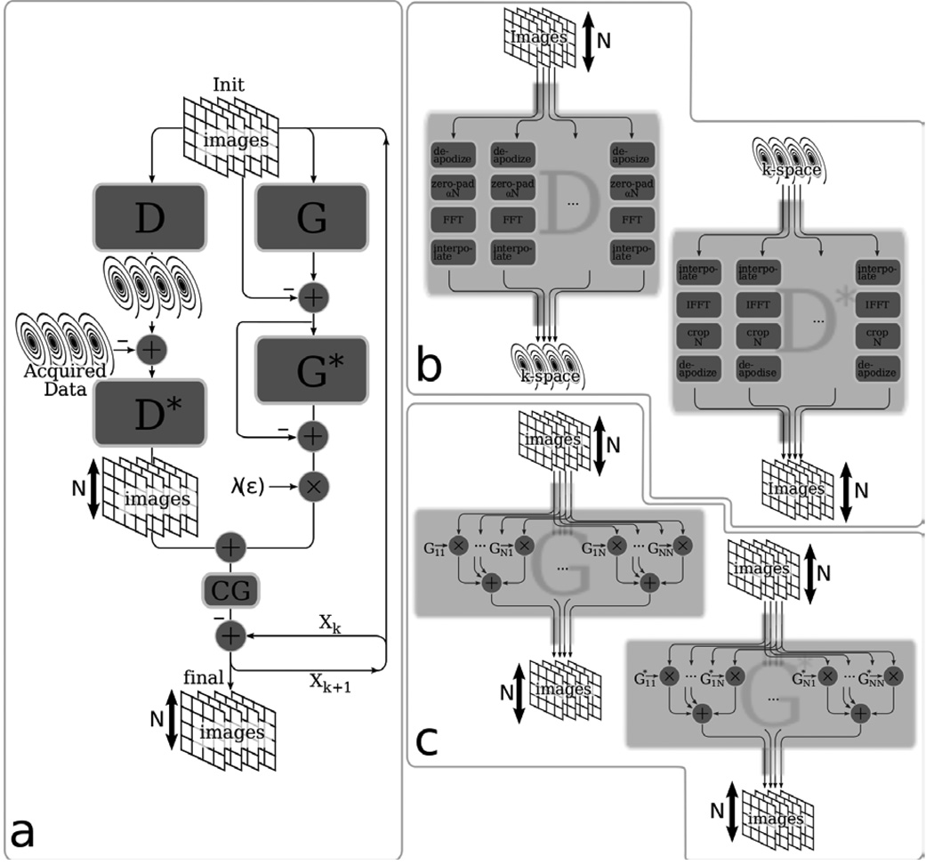
The advantage here is that large calibration kernels do not incur further increase in computational complexity since the convolution is implemented as a multiplication in image space. Figure 3 illustrates the conjugate gradient reconstruction of [Eq. 16], and the implementation of the D and G operators. The algorithm flow is similar to the k-space implementation, except for a few details. The D and D* operators perform the inverse-gridding and gridding algorithms and the G and G* operators perform image multiplications instead of convolutions. Another difference is that after the CG iterations converge, the result is the reconstructed images and no further processing is required.

Figure 3.

Image-space based reconstruction. (a) Illustration of the conjugate gradient algorithm for non-Cartesian consistency constrained reconstruction in image space. (b) Illustration of the non-uniform Fourier transform operator, D, and its adjoint, D* (c) Illustration of the calibration consistency operator, G and its adjoint, G*.

Off Resonance Correction

One of the advantages of representing the reconstruction as a solution to a system of linear equations is that it is possible to easily incorporate off-resonance variation in the reconstruction. This is particularly important for non-Cartesian trajectories, where off-resonance frequencies lead to image blurring. The off-resonance correction appears in the data consistency constraint in [Eq. 16] by modifying the nuFFT operator D to include off-resonance information. Denote ϕ_n(r) to be a complex vector with unit magnitude elements. The phase of ϕ_n(r) represents the phase of the image, contributed by off-resonance at the time the sample k(n) is acquired. The part of the operator D that operates on the i ^th coil image is,

$$y_i(n)={\displaystyle \int \delta (k(n)-r)\left\{c*{\text{FFT}}_{\mathrm{\alpha }\mathrm{N}}\left(\frac{m_i{\varphi }_n}{C}\right)\right\}(r)dr.}$$ (19)

Efficient ways to implement this operator is to approximate it using a multi-frequency reconstruction approach as described by (23, 24).

Regularization

Since [Eq. 10] is described as an optimization, one can include additional terms in the objective function, as well as constraints that express prior knowledge in the reconstruction. Consider the optimization problem

$$arg\underset{\mathbf{x}}{\text{min}}{\Vert Dx-y\Vert }^2+{\lambda }_1{\Vert (G-I)x\Vert }^2+{\lambda }_{2}R(x)$$ (20)

where the function R(x) is a penalty function that incorporates the prior knowledge. This formulation is very flexible because the penalty can be applied on the image as well as k-space data. Denoting W as a data weighting function, ∇{} as a finite-difference operator, and Ψ{} as a wavelet operator, here are some examples of potential penalties:

$$\begin{array}{lll}R(x)\hfill & =\hfill & {\Vert x\Vert }_2,\text{ Tikhonov regularization}\hfill \\ R(x)\hfill & =\hfill & {\Vert Wx\Vert }_2,\text{ Weighted Tikhonov regularization}\hfill \\ R(x)\hfill & =\hfill & {\Vert \nabla \{IFFT(x)\}\Vert }_1,\text{ Total Variation }(\text{TV})\hfill \\ R(x)\hfill & =\hfill & {\Vert \mathrm{\Psi }\{IFFT(x)\}\Vert }_1,{\ell }_1\text{wavelet}.\hfill \end{array}$$

The last two are ℓ₁ penalties and are increasingly popular due to the theory of compressed sensing (25).

Results

All the reconstructions were implemented in Matlab (The MathWorks, Inc., Natick, MA, USA). The image-based non-Cartesian reconstruction used Jeffery Fessler’s NUFFT code (22). The ℓ₁ Wavelet regularized reconstruction used David Donoho’s Wavlab code (26). The conjugate-gradient algorithm used was LSQR (27). In the spirit of reproducible research (28) we provide a software package to reproduce some of the results described in this paper. The software can be downloaded from http://www.eecs.berkeley.edu/~mlustig/software/.

Noise and Artifacts Measurements

To evaluate the noise and reconstruction properties of SPIRiT in comparison to the original GRAPPA method, we constructed the following experiment: We repeatedly scanned an axial 2D slice of a watermelon 100 times using a balanced-steady-state-free-precessession(b-SSFP) sequence with scan parameters TE = 2.5 ms, TR = 6.4 ms, flip = 60°, BW = 62.5 KHz. The slice thickness was 5 mm, field of view of 16.5 × 16.5 cm and a matrix size of 256 × 256 corresponding to 0.65 × 0.65 mm in-plane resolution. The scan was performed on a GE Signa-Excite 1.5T scanner using an 8-channel receive only head coil. To compensate for temporal phase drift between scans a 4^th order complex polynomial was fitted and removed from each pixel time-course. To compensate for the readout filter roll-off, the images were cropped to 246 × 246 pixels from which a 100 2D k-space data-sets were synthesized by computing a Fourier transform for each (complex valued) image. Each k-space data set was then undersampled uniformly by a factor of 4 (2 × 2 in each dimension) while keeping a fully sampled 24 × 24 area for calibration.

The data were processed in the following way: Each dataset was reconstructed several times using traditional GRAPPA, each time with a different kernel size (5 × 5, 7 × 7 and 9×9). The GRAPPA kernels were calibrated for each unique local sampling pattern set. In addition, each dataset was reconstructed using the k-space-based Cartesian SPIRiT with equality data consistency of [Eq. 12] again with 5 × 5, 7 × 7 and 9×9 kernel sizes. The SPIRiT reconstruction was implemented using the LSQR (27) conjugate gradient algorithm. To show the dependency of the reconstruction on the number of iterations, the results at the 6^th, 8^th, 10^th, 12^th and 14^th were saved. Finally, each dataset was reconstructed with SPIRiT with ℓ₁-norm wavelet regularization. The wavelet regularization parameter was empirically set to 0.015. For each of the above experiments, the resulting reconstructed coil images were combined with square root of sum-of-squares. Following the reconstructions, the mean difference error with the fully sampled data set was calculated. In addition the standard deviation for each pixel across the 100 scans was computed and normalized by the standard deviation of the pixels in the full set (taking into account the reduced scan time) to obtain empirical noise amplification (g-factor maps) estimates.

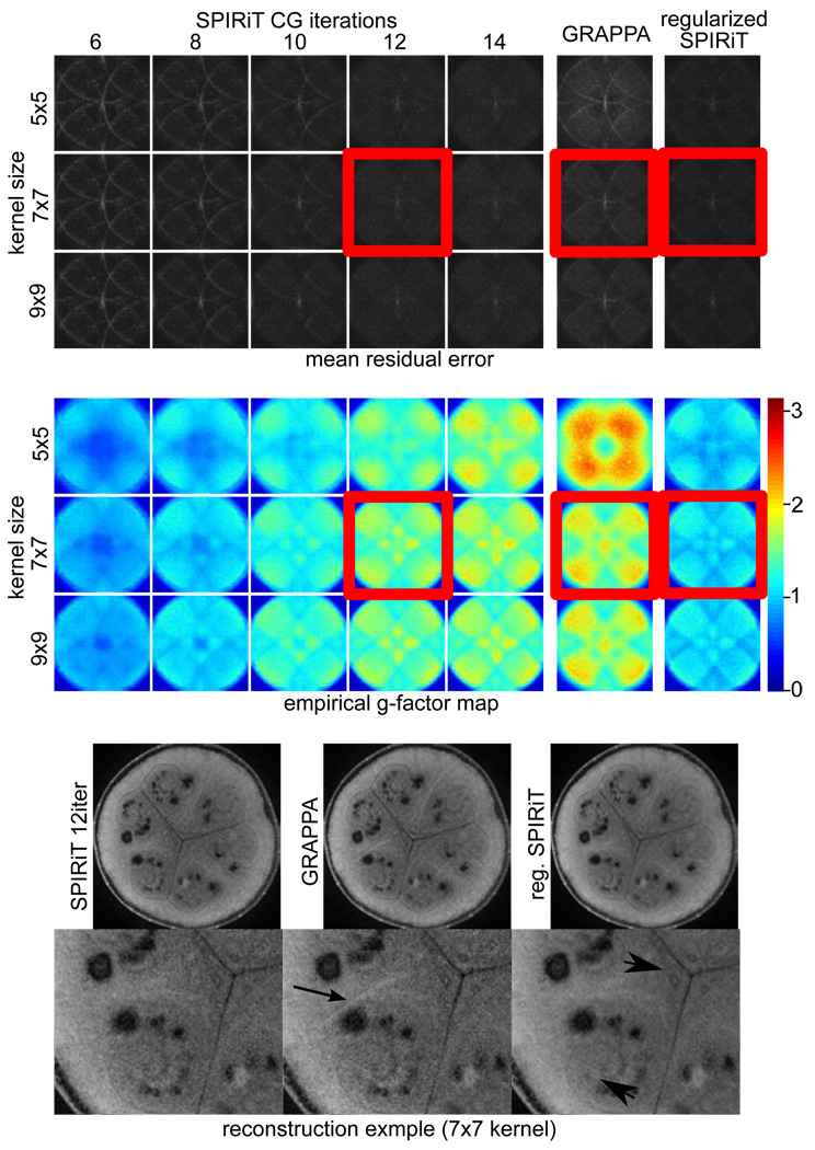
Figure 4a–c show the results of the experiments. Figure 4a 1–5 left columns show the residual error in the SPIRiT reconstruction as a function of kernel size and number of CG iterations. Overall the reconstruction is insensitive to the kernel size, achieving similarly low residual in all cases (after sufficiently number of iterations) with slightly more accurate results for the larger kernel sizes. The iterations seem to converge slightly faster for larger kernel sizes as well. The sixth column shows the residual GRAPPA reconstructions for the different kernel sizes. The reconstruction shows reduction in the residual with larger kernel size, however, the residual is significantly larger than all the SPIRiT reconstructions. The seventh column shows the ℓ₁-wavelet regularized SPIRiT residual for all the kernel sizes. They exhibit slightly lower residual similar to the non-regularized SPIRiT, which means that the regularization does not harm the accuracy of the reconstruction.

Figure 4.

Empirical reconstruction error and noise amplification maps of SPIRiT, GRAPPA and ℓ₁-wavelet regularized SPIRiT obtained from 100 scans using 8 channels and 4-fold acceleration (a) The mean residual of SPIRiT as a function of kernel size and number of CG iterations show convergence around 10–12 iterations and overall insensitivity to kernel size. GRAPPA exhibits larger residuals than SPIRiT, especially for smaller kernel sizes. The ℓ₁-wavelet regularization does not reduce the accuracy of the reconstruction (e.g., does not introduce image blurring). (b) The empirical g-factor maps demonstrate the inherent regularization and noise reduction in early termination of CG. SPIRiT exhibits an overall lower noise amplification than GRAPPA for similar residual error. The ℓ₁-wavelet regularization exhibits almost no noise amplification at all. (c) Reconstruction example. The black arrow point to residual aliasing in GRAPPA that is absent in SPIRiT. The arrowheads point to significant noise reduction in the ℓ₁-wavelet regularized SPIRiT.

Figure 4b shows the empirical g-factor maps. Figure 4b 1–5 left columns show the noise maps in the SPIRiT as a function of kernel size and number of CG iterations. It shows that as the solution becomes more accurate, the noise in the reconstruction is increased. At some point, (10–12 iterations) it is worthwhile to terminate the reconstruction as the CG iterations start fitting the noise. The figure also shows that the noise amplification in SPIRiT is lower than in GRAPPA. This is because the algorithm uses the data more efficiently and also because of the early termination of the CG iterations. The seventh column shows that the ℓ₁-wavelet regularized SPIRiT has almost no noise amplification with g-factor less or equal to one in most locations. This reconstruction offers the advantage of eliminating the g-factor without trading-off reconstruction accuracy or resolution.

Figure 4c shows a reconstruction example corresponding to the residual error and empirical g-factor maps that are marked by red boxes. The black arrow shows some residual aliasing in the GRAPPA reconstruction that is absent from both the SPIRiT reconstructions. The arrowheads point out significant noise reduction without loss of detail in the ℓ₁-wavelet regularized SPIRiT.

Arbitrary Cartesian Sampling

The SPIRiT reconstruction can easily cope with arbitrary sampling patterns. In addition, it makes efficient use of all the acquired data in the reconstruction. This becomes important at higher accelerations where SNR efficiency and good artifact reduction become key ingredients for success. To demonstrate these qualities we performed the following experiments. A T₁ weighted, inversion recovery prepared 3D SPGR sequence was used to obtain a fully sampled high resolution data set of a brain of a healthy volunteer. The scan parameters were TE = 8 ms, TR = 17.6 ms, flip = 20°, BW = 6.94 KHz. The field of view was 20 × 20 × 20 cm and a matrix size of 200 × 200 × 200 corresponding to isotropic 1 mm³ resolution. The scan was performed on a GE Signa-Excite 1.5T scanner using an 8-channel receive coil.

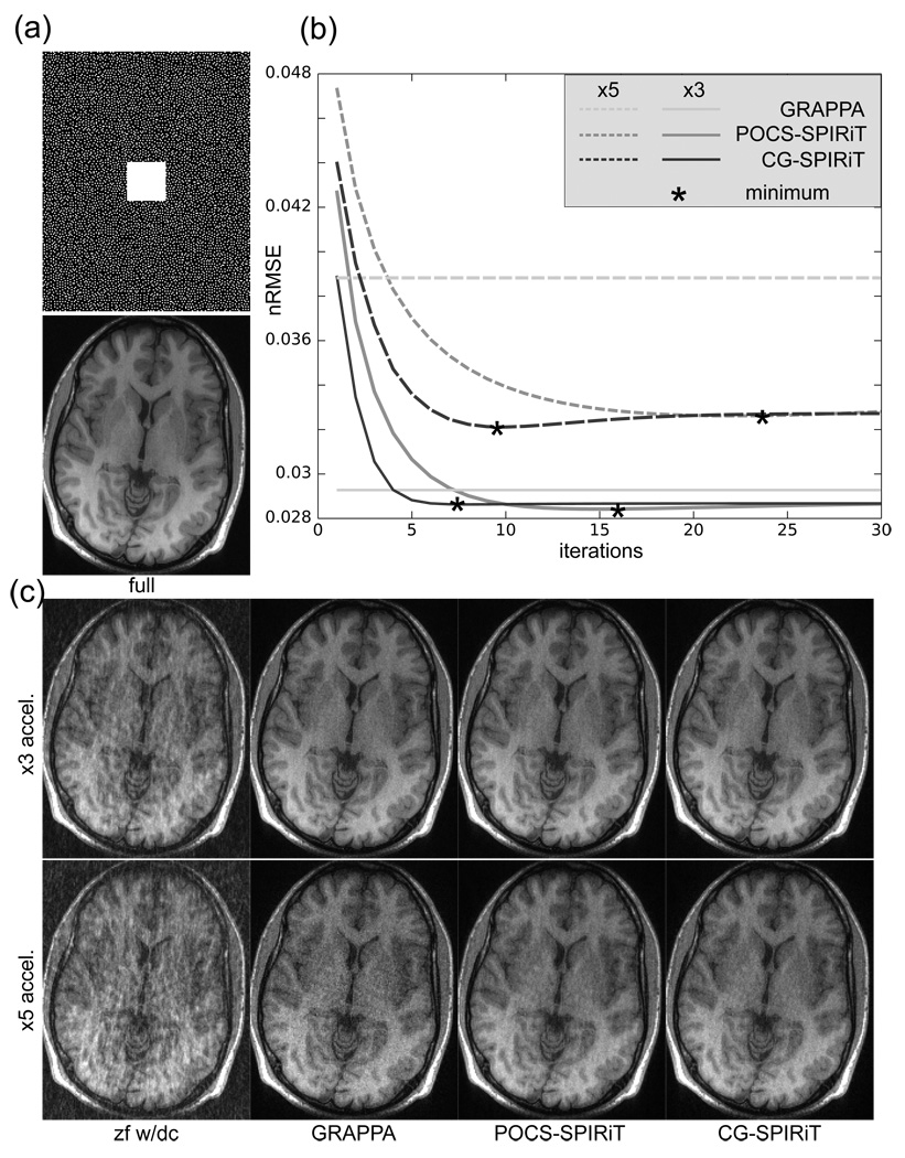
A single slice of this data set was chosen for the experiment. Two undersampling patterns were designed by choosing samples according to a Poisson-Disc sampling density (29). One data set was undersampled by a factor of 3 and the second by a factor of 5. A fully sampled area of 30 × 30 samples was left in the center of k-space for calibration. An example of the 5-fold accelerated sampling pattern is shown in Fig. 5b. The undersampled datasets were reconstructed using Cartesian GRAPPA, POCS Cartesian SPIRiT and CG Cartesian SPIRiT followed by a square-root of sum of squares combination of the coil images. Following the reconstruction, the normalized root mean squared error with the fully sampled reference was calculated using the formula $\text{nRMSE}=\frac{1}{\text{max}(x)-min(x)}\sqrt{\frac{1}{N}{\displaystyle {\sum }_{i=0}^{N-1}{(x(i)-\tilde{x}(i))}^2}}$ The SPIRiT and the GRAPPA reconstructions used a 7 × 7 size kernel.

Figure 5.

CG-SPIRiT and POCS-SPIRiT from 3-fold and 5-fold arbitrary Cartesian sampling using 8 channels. (a) 5-fold acceleration poisson-disc density sampling pattern and the reconstruction from the full data (b) Normalized RMSE (nRMSE) as a function of iterations. The advantage of SPIRiT shows at higher acceleration where efficient use of the acquired data becomes crucial. (c) Examples of the various reconstruction. Note the reduction in noise and artifacts in the SPIRiT reconstructions from 5-fold accelerated data.

Figure 5a shows the reconstruction from the full data as well as the 5-fold accelerated sampling pattern. Figure 5b shows plots of the nRMSE of the reconstructions as a function of iterations. The solid and dashed lines correspond to the 3-fold and 5-fold accelerated acquisitions respectively. The minimum nRMSE is marked by asterix. Figure 5c shows example of the reconstructions. At 3-fold acceleration all reconstructions perform similarly well and are capable of reconstructing good quality images from the undersampled data. The SPIRiT reconstructions have only slightly lower nRMSE than GRAPPA. This is because that at 3-fold acceleration with 8 channels, the reconstruction is well conditioned. At higher acceleration, where each data measurements counts, the difference in the reconstruction becomes more significant. The SPIRiT reconstructions at 5-fold acceleration have about 18% better nRMSE than the GRAPPA reconstruction. The difference in noise amplification and artifact suppression becomes much more apparent in the reconstructed images. Other details that are worth mentioning are that CG-SPIRiT converges faster than POCS with 8 iterations for CG and 16 iterations for POCS at 3-fold acceleration and with 10 iterations for CG and 24 iterations for POCS at 5-fold acceleration. However each POCS iteration is computationally cheaper than each CG iteration. The regularization property of early termination of CG is also apparent in Fig. 5b where after some iterations the error starts increasing as noise is being fitted. It is important to note that the nRMSE is not always a decreasing function because it is the normalized energy of the difference between the reconstruction and the original acquired data (which is normally not given). It should not be confused with the residual of the objective function, which is non-increasing.

Phantom Non-Cartesian Reconstruction

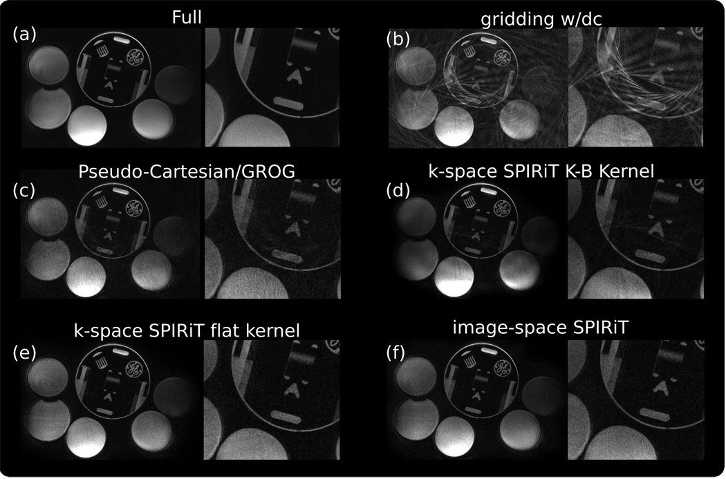
To demonstrate non-Cartesian SPIRiT reconstruction, we scanned a phantom using a spiral gradient echo sequence. The phantom chosen contains sharp edges and many image voids which make it particularly difficult to estimate sensitivity maps and therefore is ideal for an autocalibrating reconstruction. The spiral trajectory was designed with 60 interleaves, 30 cm field of view, and 0.75 mm in-plane resolution. The readout time was kept short, only 5 ms, to avoid off-resonance effects. The scan was performed on a GE Signa-Excite 1.5T scanner using a 4-channel cardiac coil. A reconstruction from the full data-set is shown in Fig. 6a.

Figure 6.

Non-Cartesian SPIRiT reconstruction from 3-fold undersampled spirals and 4 channels. (a) Reconstruction from fully sampled data. (b) Gridding with density compensation (c) Pseudo-Cartesian GRAPPA /w GROG (d) k-space SPIRiT with Kaiser-Bessel interpolator kernel (e) k-space SPIRiT with flat pass band interpolator kernel (f) Image-space SPIRiT

First, a Cartesian calibration area (32×32) was reconstructed from the full data set. These Cartesian k-space data were used to calibrate the SPIRiT kernel and also the GROG and Pseudo-Cartesian GRAPPA (16) kernels. Then, the dataset was undersampled by a factor of 3 by choosing 20 out of the 60 interleaves.

In this experiment we performed several different reconstruction. Our aim was to evaluate the quality of the image-domain and k-space domain SPIRiT methods, to demonstrate the importance of using flat-pass-band kernel for the k-space SPIRiT and to compare to existing reconstructions. We performed five reconstructions corresponding to Figs 6b–f: (b) The standard gridding reconstruction with density compensation shows, as expected, significant aliasing artifacts. (c) A Pseudo-Cartesian/GROG reconstruction was provided for us by the courtesy of Dr. Nicole Seiberlich. It used GROG to grid the data, and then pseudo-Cartesian GRAPPA with 6 source points for each pattern with an overall of 249 patterns. The reconstruction is able to reduce the artifacts, however, aliasing artifacts are still visually apparent and noise is increased. This is because this method performs parallel imaging twice. Once in the gridding stage and once in the unaliasing stage. Since the number of coils is relatively small, artifacts in one are propagated and amplified in the other. (d) The k-space SPIRiT with Kaiser-Bessel kernel parameters were: K-B kernel width=7pixels, 1.25 grid oversampling, 7 × 7 SPIRiT kernel size, 15 CG iterations. The reconstruction exhibits some residual artifacts due to the inconsistency introduced by the image weighting of the K-B interpolator. (e) The flat pass-band kernel was designed by modifying the numerical optimization by Beatty (21). The design criteria were: width=7pixels, 0.25 pass-band ripple, 0.005 stop-band ripple and 1.25 grid oversampling. In addition, a 7 × 7 SPIRiT kernel size was used and 15 CG iterations were performed. The reconstruction exhibits significant reduction of artifacts compared to the previous reconstruction. (f) The image-based SPIRiT used Fessler’s min-max NUFFT with ×2 grid oversampling. A 7 × 7 SPIRiT kernel, implemented as image multiplications was used and 15 CG iterations were performed. The reconstruction exhibits slightly better artifact suppression than the k-space method. In the Matlab implementation the reconstruction time of the k-space and image-space methods was similar. The value for λ in the non-Cartesian SPIRiT reconstructions was chosen using an L-curve analysis to be λ = 1.

In vivo Non-Cartesian Reconstruction

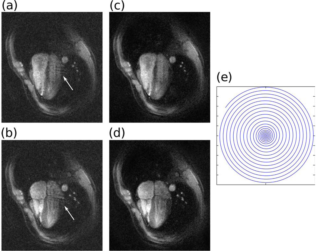
To demonstrate the image-based non-Cartesian reconstruction in-vivo we performed a dynamic heart study using a 3 interleaves dual density spiral gradient-echo sequence. The spiral trajectory was designed to support field of view ranging from 35 cm in the center to 10 cm (3-fold acceleration) in the periphery. The in-plane resolution was 1.5 mm with readout time of 16 ms, slice thickness was 5 mm. The TR was set to 25 ms achieving a sliding window temporal resolution of 40 FPS. The trajectory is illustrated in Fig. 7e. The scan was performed using the rtHawk real-time MRI system (30) installed on a GE Signa-Excite 1.5T scanner with a 4-channel cardiac coil. The data for each sliding window image was reconstructed using the image based SPIRiT algorithm. To speed up the reconstruction the previous image was used as an initial image for the reconstruction of the next image frame. This way, 7 conjugate gradient iterations were sufficient for good image quality.

Figure 7.

Dynamic cardiac imaging with dual density spirals with 3-fold acceleration and 4 channels. Two phases of a four chamber view of the heart. (a)–(b) Sum-of-squares of gridding reconstruction exhibits coherent (arrows) and incoherent (noise-like) aliasing artifacts. (c)–(d) Both the coherent and incoherent artifacts are removed by SPIRiT. (e) One out of the three spiral interleaves.

Figure 7 shows two frames in the cardiac cycle. The gridding reconstruction images (a) and (b) suffer from coherent (arrows) and incoherent artifacts due to the undersampling. These artifacts are removed by SPIRiT.

Off Resonance Correction

To demonstrate the iterative multi-frequency off-resonance correction capabilities of the reconstruction we applied the same scan parameters as in the previous section to a short axis dynamic view of the heart. Prior to the acquisition a field map measurement was taken. As a data consistency operator we used the approach described by Sutton (24).

Figure 8 shows the result of off-resonance corrected SPIRiT compared to a gridding reconstruction with no off-resonance correction. SPIRiT is able to suppress the coherent and incoherent aliasing, as well as deblurring the image.

Figure 8.

Dynamic cardiac imaging with dual density spirals and off-resonance correction with 3-fold acceleration and 4 channels. Two phases of a short axis view of the heart. (a)–(b) sum-of-squares of gridding reconstruction exhibits coherent (arrows), incoherent (noise-like) aliasing artifacts and blurring due to off-resonance. (c)–(d) SPIRiT reduces both the coherent and incoherent artifacts as well as deblurring the image (arrows).

ℓ₁-norm Wavelet Regularization

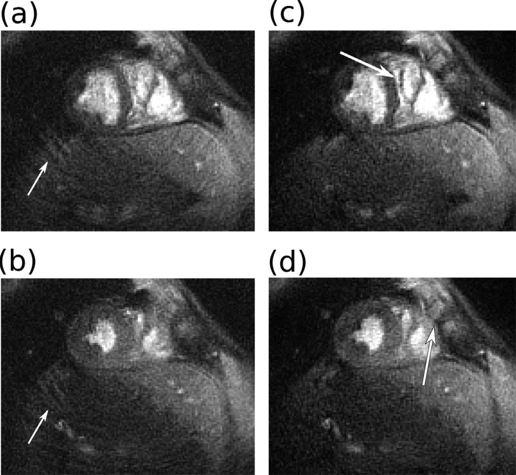
To demonstrate the regularization capabilities of SPIRiT, we performed a post contrast 3D spoiled gradient echo scan using a 12 channel body coil. The TR was 3.3 ms with a flip angle of 15 degrees. The FOV was set to 35 cm with image matrix of 192 × 192 × 88 readout, phase encodes and slice encodes respectively. Images were reconstructed using standard 2D GRAPPA parallel imaging reconstruction. Images were also reconstructed using SPIRiT with ℓ₁ wavelet (Daubechies 4) regularization.

Figure 9 illustrates the result of the reconstructions. It shows that the non-regularized 2D GRAPPA reconstruction exhibits increased noise, especially in the center of the image, due to the g factor. This noise is suppressed by the ℓ₁ regularized SPIRiT reconstruction, while the edges and features in the image are preserved.

Figure 9.

ℓ₁ wavelet regularization of 4-fold accelerated post-contrast abdomen scan with a 12 channel body coil (a) the non-Regularized GRAPPA reconstruction exhibits noise amplification due to the g factor, especially in the middle of the image. (b) Zoomed in GRAPPA reconstruction. (c) The noise amplification is suppressed in the ℓ₁ wavelet regularized SPIRiT reconstruction, while the edges and features in the image are preserved. (d) Zoomed in ℓ₁ wavelet regularized SPIRiT reconstruction.

Discussion

There are several possible extensions to SPIRiT. The SPIRiT reconstruction offers better noise performance than GRAPPA. However, optimization of the kernel for even better noise performance is possible. For example, one can use a similar scheme as (31) to optimize the kernel calibration. In addition to optimizing the kernel for noise, one can optimize noise performance by including noise covariance matrices in the SPIRiT reconstruction similarly as described in (4).

As an iterative reconstruction, the computational complexity of SPIRiT can be more intensive than direct reconstruction, especially for simple cases such as uniform undersampling. The Cartesian POCS algorithm requires in each iteration an operation similar to a single GRAPPA reconstruction. The algorithm often requires somewhere between 10 to 40 iterations to converge. The CG Cartesian algorithm requires two GRAPPA type operations per iteration. However, it is more flexible, more stable and often converges faster (6–20 iterations) than the POCS algorithm. In general, we tend to prefer the CG approach over POCS, however, the simplicity of POCS is attractive conceptually and also in implementation. The CG non-Cartesian algorithm requires two GRAPPA type operations and two gridding operations (for each coil) per iteration.

The SPIRiT approach has an advantage in reconstructions from highly non-uniform sampling patterns. In traditional GRAPPA reconstruction from such sampling schemes there is a need to perform calibration for numerous sampling patterns. For example, in the poisson-disc sampling pattern presented earlier, there were approximately 25000 individual patterns). The calibration stage for SPIRiT is negligible because SPIRiT uses only a single pattern. In such cases, the difference in reconstruction times may be significantly reduced.

Although our results comparing the k-space domain and image-domain non-Cartesian SPIRiT are not conclusive, we tend to prefer the image-domain approach and find it easier to use for several reasons: The choice of parameters in the image-domain approach is straightforward; the gridding algorithm is unchanged, the choice of the SPIRiT kernel size is the same as Cartesian SPIRiT and is independent of the the gridding parameters. On the other hand, in the k-space approach, the gridding has an additional pass-band ripple parameter in the kernel design and the tradeoffs are less obvious because the choice of grid oversampling affects the SPIRiT kernel size. In addition to all the above, if image-based regularization is used (and it should be used!) then the image-domain approach is natural and much more efficient.

In all our experiments the SPIRiT reconstruction had better noise performance than other GRAPPAlike algorithms, especially when the acceleration is pushed to the limit. This is mostly because SPIRiT uses the acquired data more efficiently. SPIRiT uses a small local kernel in k-space. However, because of the the SPIRiT operation is repeated in every iterations, the “information” propagates in k-space and acquired data in one location of k-space affects the reconstruction of k-space locations far beyond the kernel radius. This has a averaging effect of noise, and the overall noise is reduced.

Conclusions

We have presented SPIRiT, a self consistency formulation for coil-by-coil parallel imaging reconstruction. The reconstruction can be solved efficiently using iterative methods for data acquired on arbitrary k-space trajectories. We presented two variants of the reconstruction; image-domain, and k-space domain. In the k-space domain reconstruction we introduced new requirements for k-space interpolation. In addition, we demonstrated that the formulation is easily extendible to include other techniques such as regularization and off-resonance correction. We showed that enforcing consistency constraints results in better conditioning, more accurate reconstruction, and better noise behavior than the traditional GRAPPA-like approaches.

References

- 1.Roemer PB, Edelstein WA, Hayes CE, Souza SP, Mueller OM. The NMR phased array. Magn Reson Med. 1990;16:192–225. doi: 10.1002/mrm.1910160203. [DOI] [PubMed] [Google Scholar]
- 2.Kelton JR, Magin R, Wright SM. An algorithm for rapid image acquisition using multiple receiver coils; Proc., SMRM, 8th Annual Meeting; Amsterdam. 1989. p. 1172. [Google Scholar]
- 3.Sodickson DK, Manning WJ. Simultaneous acquisition of spatial harmonics (SMASH): Fast imaging with radiofrequency coil arrays. Magn Reson Med. 1997;38:591–603. doi: 10.1002/mrm.1910380414. [DOI] [PubMed] [Google Scholar]
- 4.Pruessmann KP, Weiger M, Scheidegger MB, Boesiger P. SENSE: Sensitivity encoding for fast MRI. Magn Reson Med. 1999;42:952–962. [PubMed] [Google Scholar]
- 5.Pruessmann KP, Weiger M, Börnert P, Boesiger P. Advances in sensitivity encoding with arbitrary k-space trajectories. Magn Reson Med. 2001;46:638–651. doi: 10.1002/mrm.1241. [DOI] [PubMed] [Google Scholar]
- 6.Kyriakos W, Panych L, Kacher D, Westin C, Bao S, Mulkern R, Jolesz F. Sensitivity profiles from an array of coils for encoding and reconstruction in parallel (SPACE RIP) Magn Reson Med. 2000;44:301–308. doi: 10.1002/1522-2594(200008)44:2<301::aid-mrm18>3.0.co;2-d. [DOI] [PubMed] [Google Scholar]
- 7.Yeh E, McKenzie C, Ohliger M, Sodickson D. Parallel magnetic resonance imaging with adaptive radius in k-space (PARS): constrained image reconstruction using k-space locality in radiofrequency coil encoded data. Magn Reson Med. 2005;53:1383–1392. doi: 10.1002/mrm.20490. [DOI] [PubMed] [Google Scholar]
- 8.Liu C, Bammer R, Moseley M. Parallel imaging reconstruction for arbitrary trajectories using k-space sparse matrices (kSPA) Magn Reson Med. 2007;58:1171–1181. doi: 10.1002/mrm.21334. [DOI] [PMC free article] [PubMed] [Google Scholar]
- 9.Blaimer M, Breuer F, Mueller M, Heidemann R, Griswold MA, Jacob P. SMASH, SENSE, PILS, GRAPPA: how to choose the optimal method. Top Magn Reson Imaging. 2004;15:223–236. doi: 10.1097/01.rmr.0000136558.09801.dd. [DOI] [PubMed] [Google Scholar]
- 10.Jakob P, Griswold MA, Edelman R, Sodickson D. AUTO-SMASH: a self-calibrating technique for SMASH imaging. SiMultaneous Acquisition of Spatial Harmonics. MAGMA. 1998;7:42–54. doi: 10.1007/BF02592256. [DOI] [PubMed] [Google Scholar]
- 11.Heidemann R, Griswold MA, Haase A, Jakob P. VD-AUTO-SMASH imaging. Magn Reson Med. 2001;45:1066–1074. doi: 10.1002/mrm.1141. [DOI] [PubMed] [Google Scholar]
- 12.Griswold MA, Jakob P, Nittka M, Goldfarb J, Haase A. Partially parallel imaging with localized sensitivities (PILS) Magn Reson Med. 2000;44:602–609. doi: 10.1002/1522-2594(200010)44:4<602::aid-mrm14>3.0.co;2-5. [DOI] [PubMed] [Google Scholar]
- 13.Griswold MA, Jakob PM, Heidemann RM, Nittka M, Jellus V, Wang J, Kiefer B, Haase A. Generalized autocalibrating partially parallel acquisitions (GRAPPA) Magn Reson Med. 2002;47:1202–1210. doi: 10.1002/mrm.10171. [DOI] [PubMed] [Google Scholar]
- 14.Beatty PJ. PhD thesis. Stanford University; 2006. Reconstruction Methods for Fast Magnetic Resonance Imaging. [Google Scholar]
- 15.Griswold MA, Kannengiesser S, Heidemann R, Wang J, Jakob P. Field-of-view limitations in parallel imaging. Magn Reson Med. 2004;52:1118–1126. doi: 10.1002/mrm.20249. [DOI] [PubMed] [Google Scholar]
- 16.Seiberlich N, Breuer F, Heidemann R, Blaimer M, Griswold MA, Jakob P. Reconstruction of undersampled non-Cartesian data sets using pseudo-Cartesian GRAPPA in conjunction with GROG. Magn Reson Med. 2008;59:1127–1137. doi: 10.1002/mrm.21602. [DOI] [PubMed] [Google Scholar]
- 17.Heidemann R, Griswold MA, Seiberlich N, Krüger G, Kannengiesser S, Kiefer B, Wiggins G, Wald L, Jakob P. Direct parallel image reconstructions for spiral trajectories using GRAPPA. Magn Reson Med. 2006;56:317–326. doi: 10.1002/mrm.20951. [DOI] [PubMed] [Google Scholar]
- 18.Heberlein K, Hu X. Auto-calibrated parallel spiral imaging. Magnetic resonance in medicine. 2006;55:619–625. doi: 10.1002/mrm.20811. [DOI] [PubMed] [Google Scholar]
- 19.Hu P, Meyer CH. Bosco: Parallel image reconstruction based on successive convolution operations; Proceedings of the 14th Annual Meeting of ISMRM; Seattle. 2006. p. 10. [Google Scholar]
- 20.Jackson JI, Meyer CH, Nishimura DG, Macovski A. Selection of a convolution function for Fourier inversion using gridding. IEEE Trans Med Imaging. 1991;10:473–478. doi: 10.1109/42.97598. [DOI] [PubMed] [Google Scholar]
- 21.Beatty PJ, Nishimura DG, Pauly JM. Rapid gridding reconstruction with a minimal oversam-pling ratio. IEEE Trans Med Imaging. 2005;24:799–808. doi: 10.1109/TMI.2005.848376. [DOI] [PubMed] [Google Scholar]
- 22.Fessler J, Sutton B. Nonuniform fast fourier transforms using min-max interpolation. IEEE Trans Signal Processing. 2003;51:560–574. [Google Scholar]
- 23.Man L, Pauly JM, Macovski A. Multifrequency interpolation for fast off-resonance correction. Magn Reson Med. 1997;37:785–792. doi: 10.1002/mrm.1910370523. [DOI] [PubMed] [Google Scholar]
- 24.Sutton B, Noll D, Fessler J. Fast, iterative image reconstruction for MRI in the presence of field inhomogeneities. IEEE Trans Med Imaging. 2003;22:178–188. doi: 10.1109/tmi.2002.808360. [DOI] [PubMed] [Google Scholar]
- 25.Lustig M, Donoho DL, Pauly JM. Sparse MRI: The application of compressed sensing for rapid MR imaging. Magn Reson Med. 2007;58:1182–1195. doi: 10.1002/mrm.21391. [DOI] [PubMed] [Google Scholar]
- 26.Buckheit J, Donoho DL. “Wavelets and Statistics”, chapter Wavelab and Reproducible Research. Berlin: Springer-Verlag; 1996. [Google Scholar]
- 27.Paige CC, Saunders MA. LSQR:An Algorithm for Sparse Linear Equations and Sparse Least-Squares. TOMS. 1982;8:43–71. [Google Scholar]
- 28.Donoho DL, Maleki A, Shahram M, Stodden V, Rahman I. Technical Report. Stanford University; 2008. 15 Years of Reproducible Research in Computational Harmonic Analysis; p. 02. [Google Scholar]
- 29.Lustig M, Alley MT, Vasanawala S, Donoho DL, Pauly JM. ℓ1-spirit: Autocalibrating parallel imaging compressed sensing; Proceedings of the 17th Annual Meeting of ISMRM, Honolulu; Hawaii. 2009. p. 379. [Google Scholar]
- 30.Santos JM, Wright G, Pauly JM. Flexible real-time magnetic resonance imaging framework. Conf Proc IEEE Eng Med Biol Soc. 2004;2:1048–1051. doi: 10.1109/IEMBS.2004.1403343. [DOI] [PubMed] [Google Scholar]
- 31.Samsonov A. On the optimality of parallel MRI in k-space. Magn Reson Med. 2008;59:156–164. doi: 10.1002/mrm.21466. [DOI] [PubMed] [Google Scholar]