A numerical strategy for efficient modeling of the equatorial wave guide

Abstract

Convection in the tropics is observed to involve a wide-ranging hierarchy of scales from a few kilometers to the planetary scales and also has a profound impact on short-term climate. The mechanisms responsible for this behavior present a major unsolved problem. A promising emerging approach to address these issues is cloud-resolving modeling. Here a family of numerical models is introduced specifically to model the feedback of small-scale deep convection on tropical planetary waves and tropical circulation in a highly efficient manner compatible with the approach through cloud-resolving modeling. Such a procedure is also useful for theoretical purposes. The basic idea in the approach is to use low-order truncation in the meriodonal direction through Gauss–Hermite quadrature projected onto a simple discrete radiation condition. In this fashion, the cloud-resolving modeling of equatorially trapped planetary waves reduces to the solution of a small number of purely zonal two-dimensional wave systems along a few judiciously chosen meriodonal layers that are coupled only by some additional source terms. The approach is analyzed in detail with full mathematical rigor for linearized equatorial primitive equations with source terms.

Convection in the tropics has a profound impact on short-term climate. Observational data indicate that tropical deep convection is organized on a hierarchy of scales ranging from cumulus clouds over a few kilometers to interseasonal oscillations over planetary scales of order 40,000 km (1–3). The mechanisms for this behavior present a major unsolved problem, despite the fact that there has been extensive research over the last few decades on these topics through parameterization of convection in general circulation models (4) as well as theory (refs. 5 and 6 and refs. therein). A particularly promising emerging approach to address these issues is cloud-resolving modeling (CRM), where idealized highly resolved two-dimensional simulations of clouds are coupled to larger-scale dynamics in a variety of ways (7–9), utilizing massively parallel computer architecture. Nevertheless, only very crude resolution of the large-scale interaction is possible with the current generation of computers. Here a hierarchy of numerical models is introduced specifically to model the feedback of small-scale deep convection on the tropical planetary waves and tropical circulation in a highly efficient manner compatible with the CRM approach. Besides its efficiency, this numerical strategy also makes a direct link with many of the observed larger-scale patterns in the equatorial wave guide such as Kelvin, Yanai, and equatorial Rossby waves (3, 10, 11), so that observations, theory, and CRM simulations can be compared in an interactive fashion.

The basic idea in the approach is to use low-order truncation in the meriodonal direction through Hermite polynomials combined with Gauss–Hermite quadrature in a meriodonal Galerkin approximation projected onto a simple discrete radiation condition. In this fashion, for example, the numerical CRM of equatorially trapped solutions symmetric about the equator at planetary scales reduces to the solution of a small number of purely zonal (i.e., two-dimensional) wave systems along a few judiciously chosen meriodonal layers that are only locally coupled by using additional source terms. Thus, there is only mild overhead to include the effects of rotation within the tropical wave guide compared with the purely zonal decoupled cloud-resolving models (7–9).

The procedure using meriodonal truncation is a systematic way to derive reduced models for the equatorial wave guide akin to the familiar well-known strategy of using multilayer models in a vertical truncation of the quasigeostrophic or primitive equations in midlatitude (11). However, the technical details are quite different and are specifically adapted to the equatorial wave guide. A simplified version of the basic meriodonal truncation strategy has been introduced recently in ref. 5 for theoretical purposes to study parameterization of convectively coupled tropical waves; the systematic use of low-order Gauss–Hermite quadrature is the key new fact that turns this basic approach into a practical numerical strategy.

The plan for the rest of this paper is the following: first, basic properties of parabolic cylinder functions, Hermite polynomials, and Gauss–Hermite quadrature are reviewed, which are necessary for the remaining developments in the paper. Next, a brief summary of the wave properties of the linearized equatorial primitive equations is presented. Then the basic Galerkin-collocation strategy is presented for a general nonlinear equation having a structure consistent with the equatorial wave guide; this formulation is general enough to include as examples the moist anelastic equations, the primitive equations, and other simplified theoretical nonlinear models for convectively coupled planetary waves with reduced vertical structure. Also the need for a simple discrete radiation condition is demonstrated here. Any cloud-resolving discretization of the (x, z) equations (7–9) can be implemented easily in the approach. Finally, the meriodonal truncation strategy is developed for the linearized equatorial primitive equations to provide a fundamental illustrative example of the approach, including both its strengths and shortcomings.

Parabolic Cylinder Functions, Hermite Polynomials, and Gauss–Hermite Quadrature

The parabolic cylinder functions are given by

1

where H_N(ξ) are the Hermite polynomials. An orthonormal basis for L² on the line is given by

2

The parabolic cylinder functions are the well-known eigenfunctions of the quantum harmonic oscillator (12, 13) and have the following properties associated with the raising and lowering operators of quantum mechanics:

3

Below, the obvious identities are utilized,

4

Next, Gauss–Hermite quadrature is introduced (13, 14). Given the Hermite polynomial, H_N(y), let y_j, j = 1, … , N, denote the N real zeroes

5

For a given N, these points y_j will define the N-meriodonal levels of the truncated model. In Gauss–Hermite quadrature, given N and the nodes y_j, 1 ≤ j ≤ N, there are positive quadrature coefficients, H̄_j, so that if one introduces the discrete inner product for functions f(y), g(y) by

6

then the discrete functions, ϕ_l(y_j), ϕ_m(y_j) are also a discrete orthonormal basis,

7

Explicit formulas for H̄_j can be found in refs. 13 and 14. In particular, for a function f(y), the L²-projection, P_Nf, is defined by

8

with f̃_j = ∫ fϕ_j dy. By combining Eqs. 6, 7, and 8, it follows that if one begins with any function f(y) satisfying P_Nf = f, then

9

The formulas in Eq. 9 show that given N, taking the discrete inner product of the ϕ_j at the discrete levels y_j with the quadrature coefficients H̄_j in the above fashion exactly reproduces the discrete values of all functions f(y) with P_Nf = f.

The Equatorial Primitive Equations

An important prototype example to test the numerical strategy developed below is given by the linearized hydrostatic equatorial primitive equations with source terms

10

Here v⃗_H = (u(x, y, z, t), v(x, y, z, t)) is the horizontal velocity field with v⃗_H^⊥ = (−v, u), w is the vertical velocity, and B is the buoyancy, with N̄ the constant buoyancy frequency. Rigid lid boundary conditions will be utilized here to mimic dynamics in the troposphere. The model in Eq. 10 already incorporates a number of key features at large scales in a CRM method for the equatorial wave guide (7–9). The CRM approach on the coarse-grained large scales would involve additional nonlinear advection terms in Eq. 10 as well as nonlinear interactive source terms, S(x, y, z, t), depending on the cloud-resolving components not given explicitly in Eq. 10 (9). The nonlinear advective terms are treated by the systematic approach in the next section, whereas the source terms require only a separate fractional step in the numerical procedure (9). Thus, the model in Eq. 10 captures a significant number of features needed in a CRM approach at large scales. This model also has the advantage that the numerical procedure developed in the next section can be analyzed explicitly in these important examples.

Under these conditions, it is well known (10, 11) that the equations in Eq. 10 reduce to a barotropic equation and an infinite number of decoupled shallow water equations,

11

where

12

and λ_q, q = 1, 2, … , with 0 < λ₁ < λ₂ < λ₃, … , are the vertical separation constants determined by the eigenvalue problem,

13

with orthonormal eigenmodes, G_q(z). The units of space and time in Eq. 10 have been nondimensionalized so that β = 1 and so that the speed of the second baroclinic mode c₂ = (N̄/λ₂), satisfies, c₂ = 1. Thus, in nondimensional units, the wave speeds c_q associated with the other baroclinic modes are given by

14

The rationale for this choice of nondimensionalization rests in the fact that a typical value of c₂ is 25 m/s (6), and it is desirable to resolve by a numerical strategy both the dry equatorial gravity waves with the speed, 50 m/s, and also the much slower convectively coupled waves (3, 5, 6) with a nearly Kelvin-wave structure with speeds of roughly 12 to 15 m/s (3, 5, 6). Of course, this choice is somewhat arbitrary and can be tuned conveniently from other considerations. The source terms, S_q(x, y, t), in Eq. 11, are expansion coefficients of the general source S(x, y, z, t) in terms of the orthonormal eigenmodes, G_q(z). The barotropic equation also has a source term determined by the vertical average of S. For simplicity in exposition, the barotropic mode contribution to Eq. 10 is omitted in the discussion here, because it can be treated separately in a different fashion.

A Low-Order Meriodonal Truncation Strategy for Numerical Modeling

Here a general meriodonal truncation strategy is formulated for a general system of equations for a vector quantity, u,

15

where A₁(u), A₂(u), B(u) are matrix-valued nonlinear functions, and L is a constant matrix. In the example of the linearized primitive equations from Eq. 10, the state vector u represents all the variables, v⃗_H, w, B, and also p.

Given N, consider the approximate solution to Eq. 15 defined through the meriodonal grid levels y_j, j = 1, … , N associated with Gauss–Hermite quadrature, i.e.,

16

Recall the operation P_N defined in Eq. 8, which involves projection on the first N, parabolic cylinder functions. The Galerkin-collocation approximation to Eq. 15 involves the approximation

17

For the moment, a precise definition of the operators on the right-hand side of Eq. 17 is postponed. With the approximations in Eqs. 16 and 17, the solution of Eq. 15 is replaced by the following approximation involving N-levels in y.

The Meriodonal Truncation Equations

18

Provided that the operators P_N(yLP_N) and P_N(∂/∂y)P_N can be computed efficiently, then the above equations are a meriodonal truncation of the equations in Eq. 15, which involves N-equations in the two (x, z) space variables alone, which are weakly coupled through these operators.

The operator P_N(∂/∂y)P_Nu is defined as follows. Given the values, u(x, y_j, z, t), from Eq. 9, P_Nu is defined by

19

With the properties in Eq. 3, one calculates

20

Thus, the explicit formula is obtained,

21

A similar calculation shows that

22

It is worthwhile mentioning that from Eq. 20 in terms of the discrete Hermite coefficients, ũ_l, 0 ≤ l ≤ N − 1, the operator P_N(∂/∂y)P_N is a skew-symmetric tridiagonal matrix with the form

23

Similarly, from Eq. 22, the operator P_NyP_N is the symmetric tridiagonal matrix,

24

With ũ_l defined from Eq. 19, the formulas in Eqs. 21 and 22 involve O(N²) explicit matrix multiplications to generate the operators P_N(∂/∂y)P_Nu and P_NyLP_Nu at the y-levels y_j for j = 1, … , N and utilize only local operations for fixed x, z, t. For fixed N, these matrices can be precomputed and called for use in the algorithm. For moderate values of N such as N = 3, 4, 5, which are sufficient to capture the large-scale symmetric and antisymmetric equatorially trapped Kelvin, Yanai, and Rossby waves, these approximations are routine to implement directly and are completely local in (x, z), because they involve processing of the meriodonal levels, u_j, j = 1, … , N for fixed (x, z, t).

There is little physical interest in using such expansions for large values of N, because the equatorial waves with large N that are significantly less trapped in the equatorial wave guide are not observed, and instead nontrivial connections to midlatitude dynamics dominate. The approximations in y developed here are akin to the pseudospectral approximations with Fourier modes familiar to the reader (15). An important difference is that no fast Fourier transform is known for the operations in Eqs. 19, 21, and 22 to reduce the operation count for large N. This is irrelevant for the developments presented here, where it is suggested that these models should be utilized only with small values of N to capture physically significant phenomena. The basic Galerkin approximation needs to be supplemented by a discrete radiation condition to not excite spurious large-scale modes that depend on N but are not equatorially trapped. Below, such a discrete radiation condition is described for the linearized equatorial primitive equations in the process of analyzing the basic algorithm presented above.

Application to the Linearized Equatorial Primitive Equations

If the basic meriodonal truncation strategy in Eq. 18 is applied to Eq. 10, by utilizing the same vertical structure equations in Eq. 13, the following approximations for the shallow water equations in Eq. 11 emerge:

25

In Eq. 25, v⃗_H = (u, v) and the superscripts denoting the qth baroclinic mode have been dropped; the reader should note from Eqs. 19–24 that all N of the y-level values v_j are coupled in Eq. 25. Here the source terms, S_q, are ignored for simplicity in exposition. To show that an explicit analysis is possible, it is useful to introduce the vectors

26

and the 3N × 3N symmetric matrix, A, defined by

27

with W̃_j = (p̃_j, ũ_j, ṽ_j). With the explicit matrices in Eqs. 23 and 24 and Eqs. 26 and 27, the meriodonal truncated approximation in Eq. 25 becomes the constant coefficient equation for the Hermite coefficients, W̃, given by

28

where B is the skew-symmetric 3N × 3N matrix given explicitly by its action on (p̃, ũ, ṽ) by

29

Recall from Eqs. 23 and 24 that ∂/∂ŷ_N is skew-symmetric, whereas ŷ_N is symmetric, so that B is necessarily an explicit skew-symmetric matrix. Thus, in terms of the discrete Hermite coefficients, W̃_j, the meriodonal truncation approximation for the linearized primitive equations has the form in Eq. 28 for any of the higher baroclinic modes with A a symmetric matrix and B a skew-symmetric matrix. This has two important implications: first, the meriodonal truncation strategy is a linearly stable numerical procedure because

30

is conserved in time. Secondly, because A is symmetric and B is skew-symmetric, Eq. 28 is a dispersive wave equation so that the dispersion relations and corresponding eigenvectors for Eq. 28 can be calculated and compared with those for the equatorial shallow water equations in Eq. 11. The analysis presented below reveals the need for an additional discrete radiation condition to supplement the basic algorithm.

Spurious Modes and a Discrete Radiation Condition

With the variables

31

and the corresponding discrete Hermite expansion coefficients, q̃_j, r̃_j, ṽ_j, the dispersion wave system from Eq. 28 above can be rewritten as the coupled equations,

32

with the convention q̃_j = r̃_j = ṽ_j = 0, j = −1, N. For the simplest case with c_q = 1, r̃_N−1, ṽ_N−1, and r̃_N−2 solve the equations

33

The first equation yields a completely spurious westward propagating “Kelvin-like” wave with a meriodonal structure strongly dependent on N, whereas the second two equations yield spurious analogues of the Yanai waves with completely incorrect phases. On the other hand, for N ≥ 2 and c_q = 1, the approximation has the attractive feature that it exactly reproduces the equatorial Kelvin wave, Yanai wave, and all equatorial Rossby and gravity waves of index M with 1 ≤ M ≤ N − 2 together with their dispersion relations (10). These facts motivate the discrete radiation conditions for general solutions of the linearized equatorial primitive equations for N-meriodonal discrete levels,

34

with the corresponding condition imposed on the source terms, S(x, y, z, t), which supplement the basic algorithm in Eq. 18 involving meriodonal truncation. Of course, these discrete radiation conditions in Eq. 34 should be applied only after the barotropic components have been removed by a straightforward vertical average.

Error Analysis for the Approximation for c_q ≠ 1

Because the algorithm exactly reproduces all the trapped equatorial waves with index M ≤ N − 2 for a given N with c_q = 1, it is obviously interesting to evaluate the errors in the algorithm for c_q ≠ 1 via the theoretical procedure sketched above. Below, such errors are reported for the values, c_q = 1/2 and c_q = 2, which correspond to dimensional Kelvin wave speeds of 12.5 m/s and 50 m/s, according to the nondimensionalization described earlier. As a more severe test case, some results are also reported for c_q = 1/4, which corresponds to a Kelvin wave speed of 6.25 m/s. Also the errors are reported here for N = 3, 4, 5 so that there are only three, four, or five meriodonal levels of truncation; the values of N = 4, 5 are small but still allow for exact resolution by the numerical algorithm for c_q = 1, the Kelvin, Yanai, and M = 1, 2 equatorial Rossby and gravity waves, which are part of the observational record (3). The case with three meriodonal levels, N = 3, is also interesting as a minimal model with Kelvin, Yanai, and symmetric, M = 1, Rossby and gravity waves.

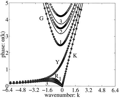
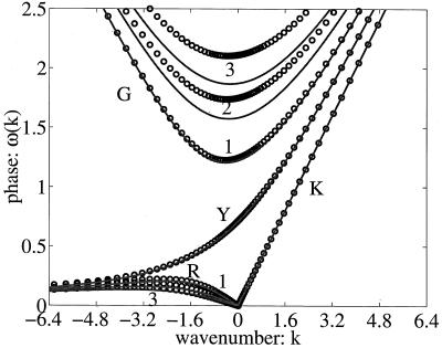
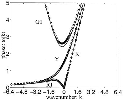
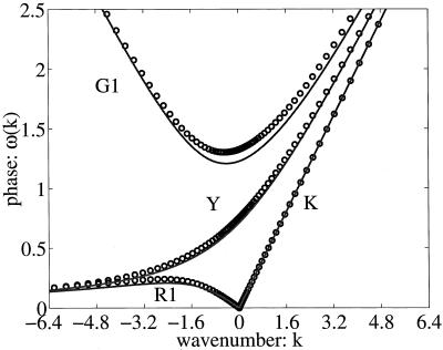
In Figs. 1 and 2, the numerical dispersion relation for N = 5 and c_q = 1/2, 2, respectively, are compared with the exact dispersion relation for the Kelvin, Yanai, and equatorial Rossby and gravity waves with M = 1, 2, 3. Clearly, the phases of the Kelvin wave are exact and the Yanai wave nearly so, with small phase errors in the Rossby waves and M = 1 gravity wave, and somewhat larger phase errors for the M = 2, 3 gravity waves. Figs. 3 and 4 depict the same approximate dispersion relation with N = 3, with similar behavior.

Figure 1.

Dispersion relations for c_q = 2 and N = 5. Solid exact solution; circles numerical solution.

Figure 2.

Dispersion relations for c_q = 1/2 and N = 5. Solid exact solution; circles numerical solution.

Figure 3.

Dispersion relations for c_q = 2 and N = 3. Solid exact solution; circles numerical solution.

Figure 4.

Dispersion relations for c_q = 1/2 and N = 3. Solid exact solution; circles numerical solution.

To quantify these errors, recall that the fundamental wave number one for the earth is given by k₁ = 2πL_e/P with P = 40,000 km and L_e = with c = 25 m/s and β = 2Ω/R; thus, k₁ = 0.16 and integer multiples of k₁ denote the higher wave numbers. The first 30 wave numbers span scales down to 1,333 km. The mean square relative error over the first 30 wave numbers in the dispersion relation for N = 3, 4, 5 and c_q = 2, 1/2, 1/4 is presented in Table 1.

Table 1.

Mean square relative error over the first 30 wave numbers in the dispersion relation

Wave	N	cq = 2	cq = 1/2	cq = 1/4
Kelvin	3	0	0	0
Yanai		0.0130	0.0280	0.1562
Rossby (M = 1)		0.1805	0.1650	0.5215
Gravity (M = 1)		0.0193	0.0402	0.2146
Kelvin	4	0	0	0
Yanai		0.0057	0.0052	0.0768
Rossby (M = 1)		0.1886	0.1650	0.5215
Gravity (M = 1)		0.0193	0.0402	0.2146
Rossby (M = 2)		0.1769	0.1935	0.2281
Gravity (M = 2)		0.0342	0.0646	0.3091
Kelvin	5	0	0	0
Yanai		0.0064	0.0052	0.0768
Rossby (M = 1)		0.1670	0.0987	0.6201
Gravity (M = 1)		0.0037	0.0078	0.0943
Rossby (M = 2)		0.1769	0.1935	0.2281
Gravity (M = 2)		0.0342	0.1935	0.3091
Rossby (M = 3)		0.1355	0.1565	0.0609
Gravity (M = 3)		0.0501	0.0876	0.3832

Note that the Kelvin wave has an exact dispersion relation, whereas the errors in the Yanai wave are small even for N = 3 and c_q = 1/4. The largest relative errors in the dispersion relation occur consistently for the Rossby waves and are between 15 and 20% for c_q = 2, 1/2; this could be anticipated, because the Rossby wave dispersion relation is nearly zero, so relative errors are exaggerated when compared with the excellent qualitative trends observed in Figs. 1–4 above.

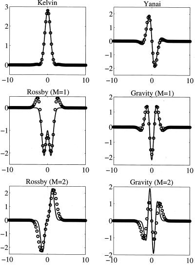
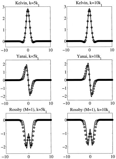
How well does the algorithm resolve the spatial structure of the equatorial waves with the accurate dispersion relation described above for N = 3, 4, 5? In Fig. 5, the meriodonal structure of pressure computed from the algorithm is compared with the exact answer for a representative wave number 5 and N = 5 for the Kelvin, Yanai, and M = 1, 2 Rossby and Gravity waves with c_q = 1/2. In Fig. 6, the same results are presented for wave numbers 5 and 10 and N = 3 for the Kelvin, Yanai, and M = 1 equatorial Rossby wave. Considering the crudeness of the approximation, the qualitative discrepancies in the meriodonal structure are not very significant.

Figure 5.

Meriodonal structure of pressure for N = 5, c_q = 1/2 and wave number 5 (k = 5k₁). Solid exact solution; circles numerical solution.

Figure 6.

Meriodonal structure of pressure N = 3 and c_q = 1/2 and wavenumbers 5 and 10. Solid exact solution; circles numerical solution.

Summary and Conclusion

A numerical algorithm designed specifically for efficient coupling of the equatorially trapped planetary waves with detailed two-dimensional cloud-resolving models (7–9) has been developed here. For the equatorial primitive equations, this algorithm amounts to the basic meriodonal truncation strategy developed in Eqs. 18, 21, and 22 combined with the readily implemented discrete radiation condition in Eq. 34 for the solution and heating sources. An explicit rigorous numerical analysis of the basic algorithm for the linearized equatorial primitive equations presented above reveals that only a small number of judiciously chosen meriodonal levels, N = 3, 4, 5, are needed to adequately represent a wide range of equatorially trapped waves, which form a significant part of the observational record (3). Detailed application of this basic algorithm for specific issues in tropical meteorology may be the subject of future research.

Abbreviation

CRM

cloud-resolving modeling

References

- 1.Nakazawa T. J Meteorol Soc Jpn. 1988;66:823–839. [Google Scholar]
- 2.Hendon H H, Liebmann B. J Geophys Res D. 1994;99:8073–8083. [Google Scholar]
- 3.Wheeler M, Kiladis GN. J Atmos Sci. 1999;56:374–399. [Google Scholar]
- 4.Emanuel K A, Raymond D J, editors. The Representation of Cumulus Convection in Numerical Models, Meteorological Monographs. Boston, MA: Am. Met. Soc.; 1993. [Google Scholar]
- 5.Majda, A. & Shefter, M. (2000) J. Atmos. Sci., in press.
- 6.Majda, A. & Shefter, M. (2000) J. Atmos. Sci., in press.
- 7.Grabowski W W, Wu X, Moncrieff M. J Atmos Sci. 1996;53:3684–3709. [Google Scholar]
- 8.Grabowski, W. W. J. Atmos. Sci. 55, 3283–3298.
- 9.Grabowski W W, Smolarkiewicz P K. Physica D. 1999;133:171–178. [Google Scholar]
- 10.Gill A E. Atmosphere-Ocean Dynamics. San Diego: Academic; 1982. , Chap. 11. [Google Scholar]
- 11.Pedlosky J. Geophysical Fluid Dynamics. New York: Springer; 1979. [Google Scholar]
- 12.Lebedev N N. Special Functions and Their Applications. New York: Dover; 1972. [Google Scholar]
- 13.Abramowitz M, Stegun I. Handbook of Mathematical Functions. New York: Dover; 1970. [Google Scholar]
- 14.Ralston A, Rabinowitz P. A First Course in Numerical Analysis. New York: McGraw–Hill; 1978. [Google Scholar]
- 15.Gottlieb D, Orszag S. Numerical Analysis of Spectral Methods. Philadelphia: Soc. Indust. Appl. Math.; 1977. [Google Scholar]