Mesh-based spherical deconvolution: A flexible approach to reconstruction of non-negative fiber orientation distributions

Abstract

Diffusion-weighted MRI has enabled the imaging of white matter architecture in vivo. Fiber orientations have classically been assumed to lie along the major eigenvector of the diffusion tensor, but this approach has well-characterized shortcomings in voxels containing multiple fiber populations. Recently proposed methods for recovery of fiber orientation via spherical deconvolution utilize a spherical harmonics framework and are susceptible to noise, yielding physically-invalid results even when additional measures are taken to minimize such artifacts. In this work, we reformulate the spherical deconvolution problem onto a discrete spherical mesh. We demonstrate how this formulation enables the estimation of fiber orientation distributions which strictly satisfy the physical constraints of realness, symmetry, and non-negativity. Moreover, we analyze the influence of the flexible regularization parameters included in our formulation for tuning the smoothness of the resultant fiber orientation distribution (FOD). We show that the method is robust and reliable by reconstructing known crossing fiber anatomy in multiple subjects. Finally, we provide a software tool for computing the FOD using our new formulation in hopes of simplifying and encouraging the adoption of spherical deconvolution techniques.

Introduction

The human brain is a phenomenally complex structure whose primary functional units, neurons, are estimated to number in tens of billions (Pakkenberg and Gundersen, 1997). Moreover, this cellular network is highly interconnected, with many neurons receiving tens of thousands of connections from sites both local and distant (Megías et al., 2001). Axons, the long cellular projections which form the anatomical basis for this neural connectivity, are organized into larger-scale fibers and fiber bundles, which are the primary constituents of the central nervous system white matter. In vivo MR imaging of this connectivity was restricted for many years to structural images (e.g. T1, T2) which provided robust discrimination of gray and white matter compartments, but conveyed no information about fiber orientation within these latter regions.

This deficiency was overcome by Basser et al. (1994a) who first demonstrated that the effective diffusion tensor at each voxel could be estimated from a series of images acquired using the pulsed-gradient spin echo (Stejskal–Tanner) sequence for diffusion-weighted imaging (DWI). The primary eigenvector of this second-order diffusion tensor has been shown, in white matter voxels, to correspond with the orientation of the fiber axis (Basser et al., 1994b). However, at current spatial resolutions, voxels are often contaminated with significant partial volume effects, and the diffusion tensor model fails to accurately represent nerve bundle geometry in voxels containing multiple fiber populations (Alexander et al., 2001; Poupon et al., 2001).

A number of high-angular resolution diffusion imaging (HARDI) approaches have been proposed which consider multiple underlying fiber orientations at each location. Here, we will focus primarily on two subsets of these methods: those which estimate the diffusion orientation distribution function (dODF), i.e., the radial projection of the spin diffusion propagator (Tuch et al., 2002; Tuch, 2004; Wedeen et al., 2005; Descoteaux et al., 2007; Aganj et al., 2009), and those for calculating the underlying fiber distribution (FOD). For a more complete overview of HARDI methods, we suggest Wu and Alexander (2007). The dODF and associated anisotropy indices (e.g., generalized fractional anisotropy) provide information about the local displacements of water molecules, which may be valuable in certain pathological states. However, for purposes of white matter architecture and tractography, we focus on estimation of the FOD, which characterizes the likelihood of a white matter bundle aligned in a given direction, as the object most directly of interest.

At each voxel, the measured DWI signal attenuation profile can be understood as the convolution of some single fiber response kernel (i.e., an impulse response) with an underlying fiber orientation distribution. Several approaches have been proposed which leverage this basic concept to address the inverse problem of recovering the FOD from a set of diffusion-weighted samples. One class of such methods aims to decompose the complex signal attenuation profile into a set of underlying 2nd-order diffusion tensors, each of which represents a single fiber population. Kim et al. (2005) achieved this goal via independent component analysis, while Peled et al. (2006) proposed a constrained two-tensor fitting process for voxels suspected of containing crossing fiber populations. Ramirez-Manzanares et al. (2007) developed a regularized procedure for combining elements from a pre-defined basis tensor set to recreate the observed diffusion tensor, thereby inferring fiber orientation via basis tensor weights. Recently, Landman et al. (2008) introduced a similar approach in which a compressed-sensing method is used to assign a sparse set of coefficients to a fixed library of prolate tensors. Also, Leow et al. (2009) assign weights over the space of symmetric positive-definite matrices to determine a tensor distribution function, from which a tensor orientation distribution can be derived to determine fiber directions.

Other related methods include the efforts to decompose the 2nd-order tensor into an isotropic and multiple purely anisotropic components (Behrens et al., 2003; Hosey et al., 2005; Behrens et al., 2007). We also recognize the process of finding the persistent angular structure (PAS) function as being conceptually similar to the deconvolution problem for fiber orientation recovery (Jansons and Alexander, 2003).

A more direct and general approach to reconstruction of principal fiber directions–one closely related to that which we propose in this work–has recently been advanced by Tournier et al. (2004). Rather than postulating a form for the impulse response, they estimate it directly from the most anisotropic voxels in the data. Using this kernel, they solve the inverse deconvolution problem directly on the sphere, S², to recover a spherical harmonic representation of the FOD at each voxel. The spherical harmonics represent a complete basis for spherical functions, analogous to the Fourier sinusoids for one-dimensional functions in that they provide a frequency-domain representation of the data. They have been utilized previously in the HARDI analysis for representation of the dODF and signal attenuation profile and offer the advantages of providing a compact representation for complex spherical data and enabling straightforward filtering techniques (Alexander et al., 2002; Anderson, 2005; Frank, 2002; Hess et al., 2006; Ozarslan et al., 2006; Descoteaux et al., 2007). Indeed, it has recently been demonstrated that a fiber orientation distribution function can be estimated, somewhat indirectly, by differential scaling of the dODF’s spherical harmonic coefficients (Descoteaux et al., 2009).

We note, however, that as a probability distribution, the FOD is subject to certain mathematical constraints—namely, it must have unit mass and be both real and non-negative over its entire domain. Furthermore, the physical interpretation of the FOD requires that it be radially symmetric if, as is commonly assumed, the minimum fiber bundle radius of curvature is much greater than the typical spin displacement during imaging and no significant migration of spins occurs between fiber bundles (i.e. the diffusion compartments are in “slow exchange”). These constraints produce some difficulties for methods which generate spherical harmonic representations of the FOD. Fundamentally, these problems stem from the fact that valid FODs exist only in the subspace of spherical functions containing real, symmetric, and non-negative functions, a space which cannot be spanned by a finite number of spherical harmonics. The more general nature of the spherical harmonic bases has necessitated the use of certain workarounds to ensure that ODF reconstructions are restricted to the valid range. Specifically, the realness of the spherical harmonic ODF reconstruction is typically enforced by using a modified real-valued basis, while the symmetry constraint is met by forcing all odd-order coefficients to be zero (Hess et al., 2006; Descoteaux et al., 2007).

The non-negativity constraint, however, has been more challenging to satisfy within the spherical harmonics framework (Tournier et al., 2004; Anderson, 2005; Tournier et al., 2007; Tournier et al., 2008). No straightforward manipulation of the spherical harmonic bases has been identified which restricts reconstructions to the nonnegative space. This criterion is rarely violated in the least-squares estimation of dODFs due to the typically large 0th degree coefficient (i.e. DC offset) needed to accurately fit the spin diffusion profile. The FOD, however, lacks this property, and the ill-posed nature of the deconvolution problem results in the frequent appearance of negative lobes in the FODs generated by previously reported methods. Common ad hoc methods for dealing with negative values in the FOD include resetting them to zero or suppressing them upon display. More recently, Tournier et al. (2007) and Tournier et al. (2008) have described a method for constrained spherical deconvolution (CSD), an iterative approach to the inverse problem which penalizes negative values in the FOD. This approach has been shown to minimize the appearance of negative regions in the FOD, but it cannot explicitly forbid them. Furthermore, an intuitive interpretation of exactly how the FOD estimate changes through the CSD iterations is somewhat lacking. Other approaches to the physically-valid spherical deconvolution include those of Alexander (2005) who has explored spherical deconvolution from a maximum entropy perspective, and Kaden et al. (2007) who parametrize the FOD by a mixture of Bingham distributions.

Here, we present an alternate approach to spherical deconvolution in which we discretize the problem onto a dense spherical mesh and solve via a projected gradient descent algorithm. In contrast to previous related works (Tournier et al., 2007, 2008), we operate in the spherical spatial domain rather than the frequency domain, avoiding the difficulties in satisfying non-negativity associated with the latter approach. In addition, we provide a clearer and more straightforward formulation, casting the constrained deconvolution as a convex optimization problem with a single cost function which, unlike those in previous methods, does not vary from one iteration to the next. We also implement the mesh-based algorithm and provide a publicly-available software tool for fiber orientation recovery via spherical deconvolution. We demonstrate that our new formulation enables stable reconstruction of the FOD while strictly satisfying the realness, nonnegativity, and symmetry requirements in a principled and predictable manner. Additionally, we include a regularization term in our method which provides for tunable noise suppression and smoothness biasing. We explore the properties of this new approach below using both simulated and real data sets, comparing its properties to ad hoc approaches for ensuring non-negativity. We find that the mesh-based approach accurately recovers simulated and known anatomical fiber orientations, and that this method is both flexible in allowing the user to determine the sharpness of the final solution and robust in that regularization parameters need not be tuned separately for each data set.

Methods

Discrete spherical mesh formulation

From a linear systems perspective, the diffusion signal attenuation profile can be viewed as the convolution of a single fiber response function with the fiber orientation distribution (FOD). In the ideal case, the signal s can thus be represented in terms of the FOD x and the kernel h:

$$\begin{array}{ll}s(\theta ,\phi )& =x(\theta ,\phi )h(\theta ,\phi )\\ & ={\int }_0^{2\pi }{\int }_0^{\pi }x\left({\theta }^{\prime },{\phi }^{\prime }\right)h\left(\theta -{\theta }^{\prime },\phi -{\phi }^{\prime }\right)d{\phi }^{\prime }d{\theta }^{\prime }\end{array}$$

Spherical deconvolution attempts to solve the inverse problem of determining x, given a limited number of noise-corrupted samples of s and a suitable estimate of h.

Recognizing that the difficulty associated with ensuring nonnegativity stems from the choice to use the spherical harmonic bases to represent the FOD, we instead derive a new formulation defined on a discrete mesh:

$$\widehat{\mathbf{x}}=\underset{\mathbf{x}}{\text{argmin}}\left({\left|\right|\mathbf{Ax}-\mathbf{y}\left|\right|}_2^2+\mathbf{\tau }{\left|\right|\mathbf{Dx}\left|\right|}_p^p\right)\text{s}.\text{t}.\mathbf{x}\ge 0,p\ge 1,{\mathbf{x}}^T\mathbf{w}=1$$ (1)

where A is the convolution matrix, x is the FOD estimate, and y contains the measured signal attenuations. This formulation characterizes a convex optimization problem in which we seek to minimize the energy function $f(\mathbf{x})={\left|\right|\mathbf{Ax}-\mathbf{y}\left|\right|}_2^2+\mathbf{\tau }{\left|\right|\mathbf{Dx}\left|\right|}_{\text{p}}^{\text{p}}$. In this manner, we define a balance between the L² norm of a data-driven term and a separate regularization term, each of which is explained in futher detail below.

The first term of the energy function, ${\left|\right|\mathbf{Ax}-\mathbf{y}\left|\right|}_2^2$, is the L² or Euclidean norm of the residual vector between the measured signal attenuations in y and the FOD estimate x transformed into this “signal attenuation space” through the convolution matrix A. Thus, this data-driven term is minimized when the estimated FOD convolves into exactly the signal attenuations measured. Note that standing alone, the L² norm of the residual embodies the ordinary least-squares problem.

The mesh-based nature of our approach is made evident in the construction of the convolution matrix A, which we define on a hemispherical icosahedral tessellation. For an icosahedral subdivision of order i, such a mesh has n=5·4ⁱ+1 unique directions on which the FOD x will be defined. For this work, we select i=4 for a 1281-point mesh. Given m directional signal attenuations, collected for each voxel in y, the convolution matrix A takes on dimensionality m×n; that is, A transforms the m-dimensional signal attenuation vector into the n-dimensional FOD estimate. Each column of A is formed by aligning the single fiber response function (i.e. the impulse response, described further below with the corresponding mesh direction and interpolating by inverse distance weighting onto the original m measurement directions. In other words, we rotate the discrete fiber response function to align with a mesh vertex, and we sample the value of this function on the original diffusion-weighting gradient directions through interpolation. Thus, if we denote the original measurement directions as u_j, the directions after rotation as ũ_j, interpolated signal attenuation s̃, and normalization constant Z, we have:

$$\stackrel{\sim }{\mathbf{s}}({\mathbf{u}}_j)=\frac{1}{Z}\sum _{j=1}^m\frac{\mathbf{s}\left({\stackrel{\sim }{\mathbf{u}}}_j\right)}{{\text{acos}}^2\mid \langle {\mathbf{u}}_j,{\stackrel{\sim }{\mathbf{u}}}_j\rangle \mid }$$ (2)

The vector s̃ is assigned to the column in A corresponding to the mesh vertex to which the kernel was aligned. This process is repeated for each point on the mesh to fill the n columns of A.

The second term in Eq. (1) provides for flexible regularization. In typical cases, the number of diffusion gradient directions measured is less than the number of mesh vertices on which the reconstruction is desired (i.e. m<n), and the deconvolution problem described by Ax=y is underdetermined. The inclusion of the regularization term allows solutions containing the properties described by D to be penalized relative to others. The parameter τ controls the relative contributions of the regularization and data-driven terms, while p indicates a p-norm level to be used in regularization.

The contraints x≥0 and x^Tw=1 are used to enforce the nonnegativity and unit mass requirements on the FOD. The n-length vector w is a weighting vector in which each element represents the amount of the total spherical surface area attributable to the corresponding vertex. Thus, ||w||₁ =4π. For a dense icosahedral mesh as we use here, these weights are very nearly equal, and the approximation which assigns each element of w to be 4π/n is justifiable. The constraint on the regularization parameter p≥1 ensures the convexity of the problem.

A number of interesting properties of this approach are evident directly from the formulation. First, by defining the deconvolution on a hemispherical mesh, symmetry of the final solution can be ensured trivially by reflection across the origin. In addition, the presence of the regularization term allows for the minimization to be guided by prior knowledge. In this report, for example, we assume that the FOD has some degree of spatial smoothness, and accordingly, we define D to be a difference matrix (weighted according to fractional mesh area) for neighboring vertices on the mesh. In this manner, we penalize large variations in the FOD between neighboring vertices. This penalty is similar in principle to the constraint function utilized by Sakaie and Lowe (2007) for FOD regularization. Finally, we note the useful property that, since Eq. (1) is convex for all p≥1, the solution x̂ is guaranteed to be globally optimal.

Projected gradient descent

Eq. (1) describes the deconvolution as a convex optimization problem. We have already noted that a symmetric solution is inherent in the formulation. The task then remains to perform the minimization in a way that ensures realness, non-negativity, and unit mass. Projected gradient descent provides a way to achieve this objective.

At each voxel, we begin by generating an initial guess for the inverse problem Ax=y. Because this problem is ill-posed, we obtain the pseudoinverse A⁺ via truncated singular value decomposition in which we retain only as many of the largest singular values as necessary to preserve 90% of the energy in A. The result is then made to satisfy the constraints x≥0 and ||x||₁ =1 by straightforward projection onto the non-negative region of the unit mass surface to provide the initial condition x₀. We next begin the iterative process of stepping along the direction of the negative gradient. If f(x) denotes the objective function to be minimized in Eq. (1), we have:

$$\nabla f(\mathbf{x})={\mathbf{A}}^{\mathbf{T}}(\mathbf{Ax}-\mathbf{y})+\mathbf{\tau }p{\mathbf{D}}^{\mathbf{T}}\left(\mathbf{Dx}·{\mid \mathbf{Dx}\mid }^{p-2}\right)$$ (3)

where the exponentiation and the multiplication indicated by (·) are element-wise operations. We perform a line search along this direction to determine the optimal step length δ, projecting the updated result onto the space of non-negative FODs with unit mass:

$${\mathbf{x}}_{\mathbf{t}}^{\prime }={\mathbf{x}}_{\mathbf{t}}-\delta \nabla f({\mathbf{x}}_{\mathbf{t}})$$ (4)

$${\mathbf{x}}_{\mathbf{t}+1}=\mathbf{P}{\mathbf{x}}_{\mathbf{t}}^{\prime }-\left(\mathbf{P}{\mathbf{x}}_{\mathbf{t}}^{\prime }·\widehat{\mathbf{w}}\right)\widehat{\mathbf{w}}$$ (5)

Here, the n×n orthogonal projection matrix P is diagonal with P_ii =0 if the ith entry of ${\mathbf{x}}_{\mathbf{t}}^{\prime }$ is negative, and P_ii =1 otherwise. ŵ, the unit-length version of the weighting vector w defined previously, is normal to the hyperplane containing all x which satisfies x^Tw=1.

The gradient is then recalculated and the process is repeated until a termination criterion is satisfied; for all experiments in this report, we chose to cease iterating when the J-divergence (symmetrized KL-divergence) between subsequent FOD estimates fell below 1×10⁻⁸, a heuristic value which will naturally depend on the choice of mesh density. Use of the J-divergence as a termination threshold ensures that the procedure continues only as long as the FOD estimate is changing significantly from one iteration to the next. The final update to the FOD is the desired solution x̂. We have summarized the entire process in Table 1.

Table 1.

Projected gradient descent algorithm.

Form an initial guess x0 via truncated SVD, projected onto the non-negative space. Calculate the gradient vector according to Eq. (3). Perform a line search along the direction of the negative gradient to determine the optimal step length δ. Update the FOD estimate x according to Eqs. (4) and (5). Repeat steps 2–4 until the J-divergence of successive FOD estimates falls below the termination threshold.

The realness of the final solution is obvious from this description; all of the terms in Eq. (1) are real, and we do not introduce any complex values through gradient descent. As for the the non-negativity constraint which has proven difficult to satisfy in the spherical harmonic framework, we observe that it is guaranteed in our mesh-based formulation. By projecting each step of the minimization onto the non-negative space, our procedure explicitly forbids any negative values in the FOD. Our projection method also ensures that the final solution satisfies the unit mass property of probability distributions. We note that projected gradient descent is a well-characterized approach to solving constrained convex optimization problems. Its performance has been widely studied, and for problems of the form (1), it has been proven to converge to the lowest energy solution which also satisfies the constraints (Iusem, 2003). Furthermore, projection has a more intuitive and less esoteric interpretation than CSD, which attempts to enforce non-negativity in the spatial domain by modifying coefficients of the frequency domain (Tournier et al., 2007, 2008). We favor this procedure for performing the spherical deconvolution as a more principled and predictable method than those previously described.

Response function estimation

All methods for performing the spherical deconvolution require a reasonable estimate of the single fiber response function to represent the convolution kernel. Implicit in this requirement are several assumptions which remain to be tested. For example, it has not been examined whether a single convolution kernel accurately models diffusion arising from fiber bundles across the entire brain which may have varying degrees of coherence or myelination. Nevertheless, we proceed cautiously as in previous reports and stipulate that the response function is constant across voxels.

We may choose either to define the fiber response function based on assumed prior knowledge or to estimate it directly from the data. We select the latter approach which has the theoretical advantage of incorporating unique features of the scanning hardware, acquisition parameters, and the subject’s anatomical characteristics into the putative kernel.

We begin by estimating the dODFs using the conventional spherical harmonic approach (Descoteaux et al., 2007). We then sample the spherical harmonic reconstruction on the chosen spherical mesh, and use these values to compute the generalized fractional anisotropy (GFA) and maximum diffusion direction for each voxel. The 300 voxels with the highest GFA are assumed to contain only a single fiber bundle and are labeled “response function voxels.” The signal attenuations from all response function voxels are aligned according to maximum diffusion direction and averaged (using inverse distance-weighted interpolation) to estimate the impulse response. Additionally, values on measurement directions which are equiangular from the maximum diffusion direction are averaged together to ensure axial symmetry.

Software

We implemented the preceding mesh-based deconvolution approach using the Java language as a module within LONI’s Pipeline environment (available for download at http://pipeline.loni.ucla.edu). The Pipeline’s modular design and substantial backend infrastructure make it an ideal tool for processing computationally intensive neuroimaging tasks (Rex et al., 2003). All of the deconvolution results in this report were generated using this tool. In the Pipeline, computational tasks are represented graphically as “workflows”; a sample workflow for mesh-based spherical deconvolution is illustrated in Fig. 1. Workflows submitted through the Pipeline are executed on a computing cluster comprised of more than 800 2.4 GHz CPUs (Dinov et al., 2009). This computational framework enables the deconvolution operation to be massively parallelized for increased processing speed.

Fig. 1.

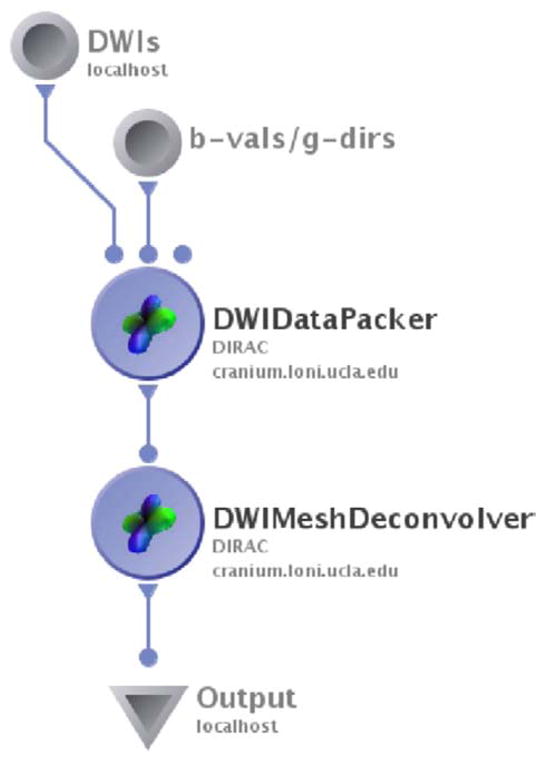
Representative workflow for mesh-based spherical deconvolution using LONI’s Pipeline.

Synthetic data simulations

For synthetic data experiments, we select the well-characterized multi-tensor model:

$$\mathbf{s}\left({\mathbf{u}}_{\mathbf{j}}\right)={\left[{\left(s_0\sum _q{f}_q{e}^{-b{\mathbf{u}}_{\mathbf{j}}^{\mathbf{T}}{\mathbf{D}}_{\mathbf{q}}{\mathbf{u}}_{\mathbf{j}}}+{\eta }_1\right)}^2+{\eta }_2^2\right]}^{\frac{1}{2}}$$ (6)

where f_q denotes the fraction contribution of the qth fiber. The prolate diffusion tensor D_q for each fiber was calculated with eigenvectors oriented along the desired directions and fixed eigenvalues: λ₁ =1.7× 10⁻³mm²/s and λ₂ = λ₃ =0.2×10 ⁻³mm²/s. The noise samples η₁ and η₂ were drawn from a zero-mean Gaussian distribution with a standard deviation determined by the desired signal-to-noise ratio: σ=1/SNR. This noise level is defined with respect to the diffusion-weighted samples as opposed to the unweighted reference (Eq. (6)). In this report, we perform all simulations at a b-value of 3000 s/mm². The gradient directions u_j were generated using an electrostatic repulsion model.

The “response function voxels” used to estimate the fiber response function for synthetic data experiments were 300 single fiber simulations generated with the same SNR as the main data set.

Data acquisition

Real data sets were acquired at the Centre for Magnetic Resonance (University of Queensland, Brisbane) using a 4 Tesla Bruker Medspec scanner (Bruker Medical, Ettingen) with a transverse electromagnetic headcoil. Diffusion-weighted scans utilized a single-shot echo planar technique with a twice-refocused spin echo sequence to minimize eddy-current induced distortions. The timing of the diffusion sequence was optimized for SNR. A total of 105 scans were acquired per subject—94 diffusion-sensitized gradient directions plus 11 baseline images with no diffusion-sensitization. Imaging parameters were: b-value= 1159 s/mm², TE/TR=92.3/8,259 ms, FOV=230 mm×230 mm, and 55×2 mm contiguous slices. The reconstruction matrix was 128×128, yielding 1.8 mm×1.8 mm in-plane resolution. Total acquisition time was 14.5 min. A single data set was acquired per subject (no averaging). Estimated SNR≈27 for the b₀ volumes, and ≈9 for diffusion-weighted volumes (noise variance was measured from non-brain regions of the image as in NEMA (2008)).

Results

Mathematical validation

We began by verifying the mathematical characteristics of our approach. For this purpose, we tested our algorithm on a 60-directional simulated data set containing two equally-weighted fibers crossing at 90° with SNR=30, τ=0.025 and p=2.00. We first demonstrate qualitatively that our approach guarantees non-negativity by comparing the deconvolution results with and without projection of the FOD estimate onto the non-negative space at each iteration. Without enabling the projection step of the algorithm (Eq. (5)), we obtain a final solution which contains negative side lobes, indicated in black in Fig. 2. Implementing the projection step eliminates these side lobes completely, validating our assertion that gradient projection is sufficient to ensure compliance with the nonnegativity constraint on the FOD. We observe that the projected FOD is slightly sharper along the true fiber directions, and in this case, we also note the presence of a small positive-valued out-of-plane (red) lobe in the unprojected FOD, which is eliminated in the projected solution.

Fig. 2.

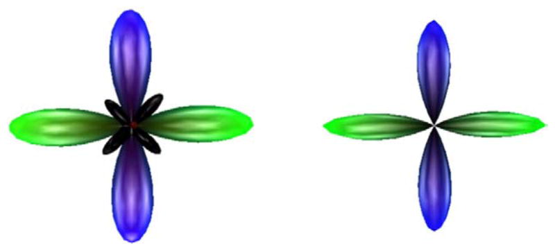
Effects of projection onto the non-negative space. Without projection (left), spherical deconvolution yields a solution containing negative-valued regions (black). Enabling projection results in elimination of these negative side lobes from the FOD solution (right). Results are for a 60-direction simulated data set modeling a 90° crossing with SNR=30, b =3000 s/mm², and regularization parameters τ=0.025, p=2.00. (For interpretation of the references to colour in this figure legend, the reader is referred to the web version of this article.)

In Fig. 2 and throughout this report, we illustrate the spherical FOD function by scaling the radial distance of each mesh point according to its FOD value. Note that we do not apply the min–max normalization that is commonly used to enhance the visual contrast of dODFs (Tuch, 2004); the FODs are inherently high-contrast over S² and we plot them without artificial enhancement. The coloring corresponds to the standard diffusion imaging convention which maps red, green, and blue to the x-, y-, and z-axes respectively.

In addition to establishing non-negativity through projected gradient descent, we examined the convexity of the problem and convergence characteristics of the algorithm. We generated 100 simulated voxels, again with crossing angle 90° and SNR=30, and performed the mesh-based deconvolution both with and without projection, as in Fig. 2, using τ=0.025 and p=2.00. To observe the convergence characteristics, the termination criterion was temporarily relaxed, and the value of the objective function, f(x), was recorded at each iteration. Fig. 3 shows the mean value of f(x) across the 100 trials at each of the first 20 iterations. As expected, we observe that the objective function decreases at each iteration, and furthermore that the rate of convergence decreases rapidly with iteration count. This behavior is consistent with the known characteristics of gradient descent-based convex optimization procedures. We also note that the magnitude of the objective function is smaller (difference at iteration 20=4.9×10⁻⁴) when we allow negative lobes to appear, relative to the projected case. This indicates that negative weights on certain mesh points permit the convolved reconstruction to slightly better match the measured data–i.e., that the global optimum for the corresponding unconstrained problem does not lie in the non-negative space–but as we have already argued, such a solution violates physical limitations on the FOD.

Fig. 3.

Convexity and convergence of mesh-based spherical deconvolution. 100 simulated crossing fiber voxels were generated with the same parameters as in Fig. 2. Top: mean (across 100 simulations) value of ${\left|\right|\mathbf{Ax}-\text{b}\left|\right|}_2^2+\mathbf{\tau }{\left|\right|\mathbf{Dx}\left|\right|}_p^p$ with respect to iteration number for FOD estimation using projected gradient descent. Bottom: convergence plot for FOD estimation with the projection step disabled.

Effects of gradient projection

Having confirmed the mathematical properties of the mesh-based approach, we next quantitatively evaluated the effects of the gradient projection operation on the FOD reconstruction. We recall that, when solved without imposing the non-negativity constraint through Eq. (5), the mesh-based formulation defines in the spatial domain essentially the same problem as others have derived in the spherical frequency domain (Tournier et al., 2004). A very common method of handling the negative lobes produced by these frequency-domain methods is simply clipping them to zero and renormalizing the FOD to unit mass. In the following comparisons, we evaluate the accuracy of FOD constructions obtained by using the full projected gradient approach relative to the ad hoc clipping scheme. Below, we refer to the solutions generated by these methods as “projected” and “clipped” FODs, respectively. To control for effects of the regularization term and the parameters chosen, our negative-lobed FODs are generated by disabling the projection step of the mesh-based deconvolution algorithm, rather than through a frequency-domain method.

We first analyzed the differences between FODs in terms of the earth mover’s distance (EMD) between the projected and clipped versions. The EMD, or Mallows distance, is a statistical metric for quantifying the difference between two probability distributions (Levina and Bickel, 2001). Informally, the EMD reports the minimum amount of “work” needed to change one distribution to match another. Given our goal of generating FODs which retain interpretability as probability densities, the EMD provides an appropriate comparison metric. We simulated a 60-directional acquisition of 1000 voxels, each containing two fibers at two different noise levels: SNR=10 and SNR=30. The orientation and crossing angle (≥5) of the simulated fibers were generated randomly. Deconvolution was performed using regularization parameters τ=0.025 and p=2.00. The EMD was computed between each simulated FOD and the ideal FOD composed of impulse functions oriented along the chosen mesh vertices.

Fig. 4 shows the results for this set of experiments. We observe that the clipped FODs are more different from the ideal case than are the projected FODs across all crossing angles at both noise levels. On average, across all angles, the EMD from the ideal case is 64.1% greater for clipped FODs than projected FODs at SNR=10, and 67.8% greater at SNR=30. For both the projected and clipped methods, the deviation from the ideal result increases as SNR worsens. The projected FODs show a 13.8% increase in EMD, on average, at SNR=10 relative to SNR=30, while EMD for the clipped FODs increases 11.3%. We further observe that the EMDs for the clipped method are more variable at each noise level than corresponding measure for the projected method. Since the ideal FOD is unchanged for the projected versus clipped comparison, this observation about the EMD suggests that the clipped FODs themselves are more variable at a given noise level than the projected FODs. Finally, we observe that, for both methods and noise levels, the EMD displays an increasing trend as the fiber crossing angle decreases. When crossing angle is reduced beyond the resolution threshold (studied further below), however, this increasing trend in the EMD is actually somewhat diminished. This behavior can be attributed to the characteristics of the EMD itself: despite the fact that two fiber peaks may no longer be distinguishable in narrow-angle FOD reconstructions, less “work” is required to change the merged fiber distribution into the ideal narrow-angle crossing distribution—in a statistical sense, the merged distribution is closer to the correct FOD.

Fig. 4.

Effects of gradient projection on FOD accuracy. 1000 two-fiber simulations were generated with random crossing angles, 60 diffusion-weighted samples, and b =3000 s/mm². All FOD reconstructions were computed with τ=0.025, p=2.00. Top-left: scatter-plot for earth mover’s distance between the ideal FOD and those reconstructed using gradient projection (blue) or those calculated without projection, after clipping negative lobes to zero (red) for simulations carried out at SNR=30. Bottom-left: the same experiment repeated with noise level SNR=10. Bottom-right: bars show mean ±1 standard deviation of earth mover’s distances from the ideal case over all crossing angles, summarized for both noise levels and both FOD computation methods. (For interpretation of the references to colour in this figure legend, the reader is referred to the web version of this article.)

We next examined the effects of gradient projection on the angular accuracy and resolution of the method. Popular tractography methods often simply extract the maxima of the FOD (or dODF) and rely on these reduced representations as error-free measures of fiber orientation. It is thus important to understand the performance of the mesh-based spherical deconvolution approach with regards to angular accuracy. We generated 1000 60-directional crossing fiber simulations at random crossing angles, as before, using SNR=30. We performed both projected and clipped versions of the mesh-based deconvolution using parameters τ=0.025 and p=2.00. Maximum fiber directions were obtained by extracting local maxima from the FOD as defined on the 1281-directional mesh. For FODs which exhibited more than two local maxima (suggesting spurious side lobes), we considered only the two directions with largest FOD magnitude; such a determination would be difficult to make in real data without prior knowledge about underlying anatomy, but here we focus purely on understanding the behavior of mesh-based deconvolution.

Fig. 5 shows the results of this experiment as scatter plots between the true and estimated crossing angles for both the projected and clipped methods. Qualitatively, we observe that the results for both cases are quite similar: the estimated crossing angles are distributed with some variance about the true crossing angles. This variance appears to increase as the true crossing angle decreases, until some resolution threshold beyond which two maxima can no longer be detected. Sample FODs calculated using the projected method are illustrated for various simulated crossing angles in the bottom of Fig. 5. We note that as the crossing angle decreases, the value of the estimated FOD increases on mesh points located in between the two true fiber directions. This effect is expected due to the finite width of the convolution kernel, and we see that below the resolution threshold, the reconstructions evolve into merged, broader FODs with only a single maximum. For a quantitative measure, we define the residual angle as the difference between the true and estimated crossing angle: i.e. θ_true − θ_est. Across all simulations in which two maxima were detected, the mean and standard deviation of the residual angle are −0.86°±2.65° for the projected method and −1.58°±2.87° for the clipped method. The minimum simulated crossing angle yielding two detectable maxima in the FOD was 39.7° for the projected method and 36.3° for the clipped method. The actual minimum reconstructed crossing angle was 39.0° for the projected method and 39.1° for the clipped method.

Fig. 5.

Effects of gradient projection on angular accuracy. 1000 two-fiber simulations were generated with random crossing angles, 60 diffusion-weighted samples, SNR=30, and b=3000 s/mm². All reconstructions used regularization parameters τ=0.025 and p=2.00. Top-left: plot of simulated crossing angle versus FOD maxima crossing angle for FODs computed using the projected gradient descent method of Table 1. Top-right: similar plot for FODs computed without gradient projection, but following clipping of negative lobes to zero. Bottom row: sample FODs for several crossing angles, computed using the projected gradient descent method.

Regularization parameter optimization

Until now, we have relied on regularization parameters τ=0.025 and p=2.00. To better understand the effects of these values on the reconstructed FOD, we varied them systematically across τ={0.005, 0.025, 0.050} and p={1.75, 2.00, 2.25}. We perfomed projected mesh-based deconvolution using each combination of parameters for 100 simulated voxels with two fibers crossing at 60° at SNR=10. We relied on 60 diffusion-sensitized directional acquisitions for each voxel. The average FOD over the 100 runs is shown for each combination of τ and p in Fig. 6. One example of the noisy signal attenuation profile is also displayed for reference. We can immediately make the general observation that despite the ill-posed nature of the deconvolution problem, the regularization term enables us to obtain a smooth 1281-directional FOD solution from 60 noise-corrupted observations. With respect to the parameters themselves, we note that the FOD estimate becomes smoother with increasing τ and decreasing p. The latter observation may seem inconsistent with the typical behavior of p-norm regularization, but it is indeed expected in this case since all of the elements in the vector Dx are necessarily less than unity—as a probability distribution, the weighted FOD values are themselves less than one, and D simply takes the difference between neighboring values on the mesh. This range of regularization parameters demonstrates that our approach is simultaneously flexible, with the ability to control the sharpness of the solution, and robust, particularly with respect to the parameter τ, which in this case produces reasonable results over a full order of magnitude. Moreover, we see that very similar FOD estimates may be obtained from different choices of τ and p, as in Fig. 6 for the pairs (τ=0.005, p=2.00) and (τ=0.025, p=2.25). Finally, we observe that the angular accuracy seems to be largely unaffected over this range of regularization parameters, though it is clear that over-regularization will adversely affect the minimum angular resolution.

Fig. 6.

Effect of regularization parameters on the deconvolution solution for a 60-directional simulated 60° fiber crossing with SNR=10 and b=3000 s/mm². FODs shown are the average reconstructions over 100 simulations. All FODs truly have unit mass; here, for easier visual comparison, they are scaled to have the same height. Left: deconvolution results for a range of τ={0.005, 0.025, 0.050} (top to bottom) and p={1.75, 2.00, 2.25} (left to right); black lines in the background provide a 60° reference angle. Right: one realization of the noisy, 60-directional simulated DWI signal attenuation profiles from which the FOD results were generated. Note that the signal attenuation has been rotated 90° relative to the FODs to show the large y-component (green) more clearly. (For interpretation of the references to colour in this figure legend, the reader is referred to the web version of this article.)

Real data experiments

We next evaluated the ability of our approach to resolve multi-fiber voxels in 94-directional real (non-simulated) data sets. Using Fig. 6 as a guide, we chose τ=0.025 and p=2.25 as a reasonable pair of regularization parameters for the analysis of these data. Fig. 7 illustrates the intersection of the corpus callosum and corticospinal tracts in one subject. We first estimated the FODs using all 94 diffusion-weighted samples and the projected gradient method (Fig. 7, bottom-left). The crossing geometry is clearly represented by the FODs in the region of intersection. We then performed the deconvolution again with 60 diffusion-sensitized directions (randomly discarding 34 diffusion-weighted images) to confirm that the method performs well even with a more commonly available number of directional samples. These FODs are shown in the middle panel of the bottom row of Fig. 7, and qualitatively agree well with those calculated from the full 94-directional data set. We computed the EMD between the FODs generated using 94 and 60 DWIs; this map is shown in the middle panel of the top row in Fig. 7. We see that reducing the number of diffusion-weighted samples causes the greatest difference in FODs in regions of low anisotropy: e.g. gray matter. We also performed the deconvolution (with all 94 samples) using the clipped method and examined the difference between the resulting FODs and those generated using the projected method (Fig. 7, right). In this case, we see that the ad hoc clipping method generates less sharp FODs and exhibits the greatest deviation from the projected case in highly-anisotropic white matter areas.

Fig. 7.

Resolution of the crossing between the corpus callosum and corticospinal tracts in a single subject. Top-left: the boxed area on the fractional anisotropy (FA) image indicates the region of FODs depicted in the bottom row. Bottom row: FODs calculated using all 94 available DWIs, with projected gradient descent (94proj, left); the same region calculated using only 60 DWIs (60proj, middle); and the same region calculated using all 94 DWIs, but without projection and after clipping of negative lobes (94clip, right). Top-middle and top-right panels contain maps of the earth mover’s distance between FOD reconstructions computed using the 94proj method and those computed using the 60proj or 94clip methods, respectively.

To illustrate the robustness of this choice of regularization parameters, we analyzed several additional data sets using the same values of τ and p. We show interesting FOD reconstructions from three different subjects in Fig. 8. In the top row, we see FODs accurately resolving the transverse pontine fibers (red) in the pons, amid bundles of ascending and descending fibers (blue). Note that many of the voxels in between the labeled regions exhibit crossing fiber geometry due to partial volume effects. In the middle row we display results from another subject, which highlight accurate reconstruction of the corpus callosum (red), cingulum (green), and fornix (cyan). Finally, in the bottom row, we show the distinct FODs in the anterior (thalamo-frontal tract, yellow) and posterior (corticospinal tract, blue) limbs of the internal capsule. A small area of the genu of the corpus callosum (red) is also visible. These results suggest that the simulated data sets provide an appropriate model for selecting regularization parameters to apply to real data sets, and that reliable FOD results can be obtained from multiple data sets without manual adjustment of regularization parameters for each case.

Fig. 8.

Robustness of regularization parameters. Deconvolution results for 3 interesting regions from 3 different subjects, all using the same regularization parameters: τ=0.025 and p=2.25. In each row, the right column contains a perspective view of the FODs in the region of interest, which is also boxed for reference in that subject’s corresponding b₀ (top) and FA (bottom) images in the left column. Top row: an axial section at the level of the pons illustrates FODs from the transverse pontine fibers (highlighted red) surrounded by ascending and descending connections to the spinal cord (blue). Middle row: a coronal section illustrating FODs in the corpus callosum (red), in close proximity to fibers in the cingulum bundles (green) and thefornix (cyan) oriented out-of-plane. Bottom row: an axial section at the level of the internal capsule illustrates the thalamo-frontal tract (yellow) in the anterior limb, and corticospinal fibers (blue) in the posterior limb. (For interpretation of the references to colour in this figure legend, the reader is referred to the web version of this article.)

Discussion

We have presented a hemispherical mesh-based formulation for spherical deconvolution to recover fiber orientations directly from DWI signal attenuations. This method has several unique characteristics, which we have highlighted in this report. It ensures that the estimated FOD will strictly satisfy the physical constraints of realness, symmetry, and non-negativity. Moreover, the final solution will have unit mass and be globally optimal, subject to constraints, with respect to the objective function embodied in Eq. (1). Our method also provides flexibility in the form of the regularization parameters τ and p, as well as in the choice of the regularization matrix D. This flexibility does not imply the lack of robustness, however, as we have shown that an appropriately-chosen set of regularization parameters can provide reasonable results for multiple data sets, both real and simulated.

The primary advantages of our mesh-based formulation are in its guarantee of physically-valid FOD reconstruction and its straightforward, well-characterized approach to obtaining these results. As noted, previous attempts have been made to minimize negative values in FOD reconstruction obtained using the spherical harmonics framework, but such efforts require an ad hoc approach which has a more obscure interpretation than the principled gradient projection method we propose here. We also note that enforcing a non-negativity criterion through the frequency domain may have an undesirable behavior because the spherical harmonic basis functions are periodic and globally supported, and thus manipulating the coefficients to diminish negative values in one region will necessarily change the FOD values over all of S². By applying the non-negativity constraint directly in the spatial domain, the mesh-based approach enables local adjustments to FOD shape without distant consequences. Moreover, even the modified spherical harmonics-based deconvolution approaches cannot completely eliminate negative values in the final solution, an important consideration for probabilistic or front-evolution-based tractography methods that sample the FOD at each step, which may be forced to invoke ad hoc logic themselves to handle such events. Moreover, as we have shown that such ad hoc methods may reduce the accuracy of the FOD, especially in regions of high anisotropy (Figs. 4 and 7, right), it is conceivable that the mesh-based spherical deconvolution approach has the potential to improve downstream tractography results and ultimately our understanding of brain connectivity.

Secondary advantages include beneficial side effects of the mesh-based representation itself. Determining the most likely fiber direction, for use in deterministic tractography, becomes trivial. Similarly, the mesh-based representation permits straightforward comparison of orientation differences between FODs in neighboring voxels, a metric which can be used to enable broader-scale spatial regularization of fiber tracts. For these reasons, and because we have not observed significant differences in angular resolution between our mesh-based approach and CSD, for example, we suggest that the mesh-based representation may expedite future analyses without sacrificing accuracy, albeit at the cost of a less compact representation.

The mesh-based approach also presents some unique challenges, particularly with regards to discretization. For the ith vertex, the value x_iw_i represents the likelihood of fibers oriented in directions which lie within some solid angle surrounding that vertex; the size of this solid angle is determined by the mesh geometry. This is similar to the interpretation of the discrete dODF in Tuch (2004). For some applications, however, it may be desirable to know the value of the FOD in any arbitrary direction. This can be obtained from piecewise linear interpolation of x on the triangulated mesh. Because x as weighted by w has unit integral over the mesh, the continuous function resulting from interpolating all arbitrary directions on S² in this manner will also have unit mass and retain the properties of a probability distribution, including non-negativity.

The maxima of the FOD, however, will always lie on the original mesh points following piecewise linear interpolation. For downstream applications such as deterministic tractography methods which rely solely on the maxima of the distribution, this raises a significant concern about possible discretization error. Here we have attempted to minimize this error by using a very dense mesh. For a 1281 point mesh, the angle between neighboring vertices is slightly greater than 4°, resulting in a maximum discretization error of approximately 2°. This represents less than one standard deviation of the error we observe in simulations, even at high SNR (Fig. 5). However, computation of the solution for a dense mesh is necessarily expensive as the convolution matrix A contains as many columns as there are mesh vertices (for the 60-directional data sets in this work, a single Pipeline CPU solves 100 voxels in just under 30 s). If possible, disregarding non-brain (or perhaps non-white-matter) voxels can reduce the computation time. We propose two additional approaches to further mitigate this burden. First, as the deconvolution operation treats each voxel independently, once the convolution matrix A is determined, the operation can be parallelized in a straightforward manner to compute multiple voxels simultaneously. This is the approach we have utilized in our Pipeline implementation. Second, one might use an adaptive re-meshing strategy where the deconvolution is carried out initially on a sparse mesh, and then again on a mesh which contains additional vertices near the previously detected maxima. Indeed, as we have observed little difference in angular accuracy and resolution between the “projected” and “clipped” methods, the mesh-based approach may not be the most economical choice for applications which make use of only the maxima of the FOD, rather than the full distribution.

The process of choosing appropriate regularization parameters also warrants further discussion. Throughout this report, we have defined D as the weighted spatial difference matrix over neighboring mesh vertices. As noted previously, however, the regularization matrix is a free parameter, and the user may select it in accordance with prior knowledge about the form of the solution. Accordingly, a seemingly obvious choice for D might be the identity, suggesting that the desired FOD is sparse. We note that this choice, along with letting p=1, converts Eq. (1) into the form commonly encountered in “compressed-sensing” methods (Candes and Tao, 2006; Donoho, 2006). While it is true that the FOD is zero over most of its support, this choice of regularization parameters, in our experience, produces appropriately-oriented, but highly noisy FODs due to the ill-posed nature of the spherical deconvolution. Furthermore, we observe that for p=2, Eq. (1) takes the classical Tikhonov-regularized form, and an explicit solution is available. Although this closed-form solution does not guarantee non-negativity, it may be useful as an initial guess for beginning projected gradient descent. Also, in this paper, we have relied on the multi-fiber simulation of Eq. (6) to select optimal regularization parameters for non-synthetic data sets. We have managed to obtain reasonable results with this approach, although this model is certainly an oversimplification of the true diffusion process (Inglis et al., 2001; Maier et al., 2001; Assaf et al., 2004). In addition, we note that, while we have tuned these parameters at the higher b-value (3000 s/mm²) used for simulation in previous works (Sakaie and Lowe, 2007; Tournier et al., 2007), we generate satisfactory results from data sets acquired at more conventional b-values (1159 s/mm²). This is likely largely a consequence of the fact that we obtain the single fiber response function by sampling each data set individually. Despite this robustness, it may be worthwhile, in some applications, to optimize the tuning for a particular data set by examining results for several values of τ and p for a few selected voxels from regions with known anatomy before computing the solution for the full volume.

We have noted a relative scarcity of clinical reports utilizing HARDI reconstructions and associated metrics, relative to those incorporating more traditional DTI analyses. No doubt this imbalance results partially from the increased technical requirements of HARDI acquisition, but also in part due to a sparsity of widely available tools for conducting such analyses. To this end, we hope that the software we have made available via the Pipeline will be of use to others in testing our spherical deconvolution approach on a variety of data sets for methodological comparisons and validations, as well as for quantitative investigations of clinical populations.

Future directions for investigation using the mesh-based formulation include analysis of more complex convex optimization methods in order to minimize computational load. Newton–Raphson methods, quasi-Newton methods, and conjugate gradient methods all have theoretical speed advantages for solving Eq. (1); it will be important to examine whether these can be realized in practice while still imposing the necessary constraints. In addition, the incorporation of more sophisticated prior knowledge into the regularization matrix D may lead to improved FOD reconstructions. Finally, we note that the mesh-based representation lends itself naturally to neighborhood-guided spatial regularization, and further exploration along may lead to improved or more robust tractography results.

References

- Aganj I, Lenglet C, Sapiro G. Odf reconstruction in q-ball imaging with solid angle consideration. Biomedical Imaging: From Nano to Macro, 2009; ISBI’09. IEEE International Symposium; 2009-July 1; 2009. pp. 1398–1401. [DOI] [PMC free article] [PubMed] [Google Scholar]
- Alexander AL, Hasan KM, Lazar M, Tsuruda JS, Parker DL. Analysis of partial volume effects in diffusion-tensor MRI. Magn Reson Med. 2001 May;45 (5):770–780. doi: 10.1002/mrm.1105. [DOI] [PubMed] [Google Scholar]
- Alexander DC. Maximum entropy spherical deconvolution for diffusion MRI. Inf Process Med Imaging. 2005;19:76–87. doi: 10.1007/11505730_7. [DOI] [PubMed] [Google Scholar]
- Alexander DC, Barker GJ, Arridge SR. Detection and modeling of non-gaussian apparent diffusion coefficient profiles in human brain data. Magn Reson Med. 2002 Aug;48(2):331–340. doi: 10.1002/mrm.10209. [DOI] [PubMed] [Google Scholar]
- Anderson AW. Measurement of fiber orientation distributions using high angular resolution diffusion imaging. Magn Reson Med. 2005 Nov;54(5):1194–1206. doi: 10.1002/mrm.20667. [DOI] [PubMed] [Google Scholar]
- Assaf Y, Freidlin RZ, Rohde GK, Basser PJ. New modeling and experimental framework to characterize hindered and restricted water diffusion in brain white matter. Magn Reson Med. 2004 Nov;52(5):965–978. doi: 10.1002/mrm.20274. [DOI] [PubMed] [Google Scholar]
- Basser PJ, Mattiello J, LeBihan D. Estimation of the effective self-diffusion tensor from the NMR spin echo. J Magn Reson B. 1994 Mar;103(3):247–254. doi: 10.1006/jmrb.1994.1037. [DOI] [PubMed] [Google Scholar]
- Basser PJ, Mattiello J, LeBihan D. MR diffusion tensor spectroscopy and imaging. Biophys J. 1994 Jan;66(1):259–267. doi: 10.1016/S0006-3495(94)80775-1. [DOI] [PMC free article] [PubMed] [Google Scholar]
- Behrens TEJ, Berg HJ, Jbabdi S, Rushworth MFS, Woolrich MW. Probabilistic diffusion tractography with multiple fibre orientations: what can we gain? Neuroimage. 2007 Jan;34(1):144–155. doi: 10.1016/j.neuroimage.2006.09.018. [DOI] [PMC free article] [PubMed] [Google Scholar]
- Behrens TEJ, Woolrich MW, Jenkinson M, Johansen-Berg H, Nunes RG, Clare S, Matthews PM, Brady JM, Smith SM. Characterization and propagation of uncertainty in diffusion-weighted MR imaging. Magn Reson Med. 2003 Nov;50(5):1077–1088. doi: 10.1002/mrm.10609. [DOI] [PubMed] [Google Scholar]
- Candes E, Tao T. Near-optimal signal recovery from random projections: universal encoding strategies? Inf Theory, IEEE Trans. 2006 Dec52(12):5406–5425. [Google Scholar]
- Descoteaux M, Angelino E, Fitzgibbons S, Deriche R. Regularized, fast, and robust analytical q-ball imaging. Magn Reson Med. 2007 Sep;58(3):497–510. doi: 10.1002/mrm.21277. [DOI] [PubMed] [Google Scholar]
- Descoteaux M, Deriche R, Knösche TR, Anwander A. Deterministic and probabilistic tractography based on complex fibre orientation distributions. IEEE Trans Med Imaging. 2009 Feb;28(2):269–286. doi: 10.1109/TMI.2008.2004424. [DOI] [PubMed] [Google Scholar]
- Dinov ID, Van Horn JD, Lozev KM, Magsipoc R, Petrosyan P, Liu Z, Mackenzie-Graham A, Eggert P, Parker DS, Toga AW. Efficient, distributed and interactive neuroimaging data analysis using the LONI Pipeline. Front Neuroinformatics. 2009;3:22. doi: 10.3389/neuro.11.022.2009. [DOI] [PMC free article] [PubMed] [Google Scholar]
- Donoho D. Compressed sensing. Inf Theory, IEEE Trans. 2006 April52(4):1289–1306. [Google Scholar]
- Frank LR. Characterization of anisotropy in high angular resolution diffusion-weighted MRI. Magn Reson Med. 2002 Jun;47(6):1083–1099. doi: 10.1002/mrm.10156. [DOI] [PubMed] [Google Scholar]
- Hess CP, Mukherjee P, Han ET, Xu D, Vigneron DB. Q-ball reconstruction of multimodal fiber orientations using the spherical harmonic basis. Magn Reson Med. 2006 Jul;56(1):104–117. doi: 10.1002/mrm.20931. [DOI] [PubMed] [Google Scholar]
- Hosey T, Williams G, Ansorge R. Inference of multiple fiber orientations in high angular resolution diffusion imaging. Magn Reson Med. 2005 Dec;54(6):1480–1489. doi: 10.1002/mrm.20723. [DOI] [PubMed] [Google Scholar]
- Inglis BA, Bossart EL, Buckley DL, Wirth ED, Mareci TH. Visualization of neural tissue water compartments using biexponential diffusion tensor mri. Magn Reson Med. 2001 Apr;45(4):580–587. doi: 10.1002/mrm.1079. [DOI] [PubMed] [Google Scholar]
- Iusem AN. On the convergence properties of the projected gradient method for convex optimization. Comput Appl Math. 2003;22 (1):37–52. [Google Scholar]
- Jansons KM, Alexander DC. Persistent angular structure: new insights from diffusion MRI data. Inf Process Med Imaging. 2003 Jul;18:672–683. doi: 10.1007/978-3-540-45087-0_56. [DOI] [PubMed] [Google Scholar]
- Kaden E, Knösche TR, Anwander A. Parametric spherical deconvolution: inferring anatomical connectivity using diffusion MR imaging. Neuroimage. 2007 Aug;37(2):474–488. doi: 10.1016/j.neuroimage.2007.05.012. [DOI] [PubMed] [Google Scholar]
- Kim S, Jeong J-W, Singh M. Estimation of multiple fiber orientations from diffusion tensor MRI using independent component analysis. Nucl Sci, IEEE Trans on. 2005 Feb52(1):266–273. [Google Scholar]
- Landman BA, Bazin PL, Prince JL. Compressed sensing of multiple intravoxel orientations with traditional DTI. Workshop on Computational Diffusion MRI; September.MICCAI; 2008. [Google Scholar]
- Leow AD, Zhu S, Zhan L, McMahon K, de Zubicaray GI, Meredith M, Wright MJ, Toga AW, Thompson PM. The tensor distribution function. Magn Reson Med. 2009 Jan;61(1):205–214. doi: 10.1002/mrm.21852. [DOI] [PMC free article] [PubMed] [Google Scholar]
- Levina E, Bickel P. The Earth Mover’s distance is the Mallows distance: some insights from statistics. Computer Vision, 2001. ICCV 2001. Proceedings. Eighth IEEE International Conference; 2001. pp. 251–256.pp. 251–256. [Google Scholar]
- Maier SE, Bogner P, Bajzik G, Mamata H, Mamata Y, Repa I, Jolesz FA, Mulkern RV. Normal brain and brain tumor: multicomponent apparent diffusion coefficient line scan imaging. Radiology. 2001 Jun;219(3):842–849. doi: 10.1148/radiology.219.3.r01jn02842. [DOI] [PubMed] [Google Scholar]
- Megías M, Emri Z, Freund TF, Gulyás AI. Total number and distribution of inhibitory and excitatory synapses on hippocampal CA1 pyramidal cells. Neuroscience. 2001;102 (3):527–540. doi: 10.1016/s0306-4522(00)00496-6. [DOI] [PubMed] [Google Scholar]
- NEMA. National Electrical Manufacturers Association Standards Publication MS 1-2008: Determination of Signal-to-Noise Ratio (SNR) in Diagnostic Magnetic Resonance Imaging 2008 [Google Scholar]
- Ozarslan E, Shepherd TM, Vemuri BC, Blackband SJ, Mareci TH. Resolution of complex tissue microarchitecture using the diffusion orientation transform (DOT) Neuroimage. 2006 Jul;31(3):1086–1103. doi: 10.1016/j.neuroimage.2006.01.024. [DOI] [PubMed] [Google Scholar]
- Pakkenberg B, Gundersen HJ. Neocortical neuron number in humans: effect of sex and age. J Comp Neurol. 1997 Jul;384(2):312–320. [PubMed] [Google Scholar]
- Peled S, Friman O, Jolesz F, Westin C-F. Geometrically constrained two-tensor model for crossing tracts in DWI. Magn Reson Imaging. 2006 Nov;24(9):1263–1270. doi: 10.1016/j.mri.2006.07.009. [DOI] [PMC free article] [PubMed] [Google Scholar]
- Poupon C, Mangin J, Clark CA, Frouin V, Régis J, Bihan DL, Bloch I. Towards inference of human brain connectivity from MR diffusion tensor data. Med Image Anal. 2001 Mar;5(1):1–15. doi: 10.1016/s1361-8415(00)00030-x. [DOI] [PubMed] [Google Scholar]
- Ramirez-Manzanares A, Rivera M, Vemuri BC, Carney P, Mareci T. Diffusion basis functions decomposition for estimating white matter intravoxel fiber geometry. IEEE Trans Med Imaging. 2007 Aug;26(8):1091–1102. doi: 10.1109/TMI.2007.900461. [DOI] [PubMed] [Google Scholar]
- Rex DE, Ma JQ, Toga AW. The LONI Pipeline processing environment. Neuroimage. 2003 Jul;19(3):1033–1048. doi: 10.1016/s1053-8119(03)00185-x. [DOI] [PubMed] [Google Scholar]
- Sakaie KE, Lowe MJ. An objective method for regularization of fiber orientation distributions derived from diffusion-weighted MRI. Neuroimage. 2007 Jan;34(1):169–176. doi: 10.1016/j.neuroimage.2006.08.034. [DOI] [PubMed] [Google Scholar]
- Tournier J-D, Calamante F, Connelly A. Robust determination of the fibre orientation distribution in diffusion MRI: non-negativity constrained super-resolved spherical deconvolution. Neuroimage. 2007 May;35(4):1459–1472. doi: 10.1016/j.neuroimage.2007.02.016. [DOI] [PubMed] [Google Scholar]
- Tournier J-D, Calamante F, Gadian DG, Connelly A. Direct estimation of the fiber orientation density function from diffusion-weighted MRI data using spherical deconvolution. Neuroimage. 2004 Nov;23(3):1176–1185. doi: 10.1016/j.neuroimage.2004.07.037. [DOI] [PubMed] [Google Scholar]
- Tournier J-D, Yeh C-H, Calamante F, Cho K-H, Connelly A, Lin C-P. Resolving crossing fibres using constrained spherical deconvolution: validation using diffusion-weighted imaging phantom data. Neuroimage. 2008 Aug;42(2):617–625. doi: 10.1016/j.neuroimage.2008.05.002. [DOI] [PubMed] [Google Scholar]
- Tuch DS. Q-ball imaging. Magn Reson Med. 2004 Dec;52(6):1358–1372. doi: 10.1002/mrm.20279. [DOI] [PubMed] [Google Scholar]
- Tuch DS, Reese TG, Wiegell MR, Makris N, Belliveau JW, Wedeen VJ. High angular resolution diffusion imaging reveals intravoxel white matter fiber heterogeneity. Magn Reson Med. 2002 Oct;48(4):577–582. doi: 10.1002/mrm.10268. [DOI] [PubMed] [Google Scholar]
- Wedeen VJ, Hagmann P, Tseng W-YI, Reese TG, Weisskoff RM. Mapping complex tissue architecture with diffusion spectrum magnetic resonance imaging. Magn Reson Med. 2005 Dec;54(6):1377–1386. doi: 10.1002/mrm.20642. [DOI] [PubMed] [Google Scholar]
- Wu Y-C, Alexander AL. Hybrid diffusion imaging. Neuroimage. 2007 Jul;36(3):617–629. doi: 10.1016/j.neuroimage.2007.02.050. [DOI] [PMC free article] [PubMed] [Google Scholar]