Rating Movies and Rating the Raters Who Rate Them

Abstract

The movie distribution company Netflix has generated considerable buzz in the statistics community by offering a million dollar prize for improvements to its movie rating system. Among the statisticians and computer scientists who have disclosed their techniques, the emphasis has been on machine learning approaches. This article has the modest goal of discussing a simple model for movie rating and other forms of democratic rating. Because the model involves a large number of parameters, it is nontrivial to carry out maximum likelihood estimation. Here we derive a straightforward EM algorithm from the perspective of the more general MM algorithm. The algorithm is capable of finding the global maximum on a likelihood landscape littered with inferior modes. We apply two variants of the model to a dataset from the MovieLens archive and compare their results. Our model identifies quirky raters, redefines the raw rankings, and permits imputation of missing ratings. The model is intended to stimulate discussion and development of better theory rather than to win the prize. It has the added benefit of introducing readers to some of the issues connected with analyzing high-dimensional data.

1. INTRODUCTION

Many statistical applications involve esoteric scientific theories. In teaching statistics, it is helpful to have interesting examples closer to the surface of public understanding. Sports statistics obviously furnish many opportunities. Another field of universal appeal is film. Websites such as IMDB now allow users to interactively rate movies. Rating itself is becoming more pervasive. The public rates books on Amazon, buyers and sellers rate each other on eBay, experts rate institutions such as universities in reputational surveys, and fans rate players for all star games. Inevitably, some dishonest raters give biased ratings for commercial reasons, and some idiosyncratic raters supply random ratings. This raises several interesting questions: (a) how can we tell the unreliable raters from the others, (b) how do we evaluate the true reputation of the items being rated, and (c) how can we predict what rating a rater will give to a new item?

In attacking these questions, we adopt a modeling approach. In contrast, previous research in the field of collaborative filtering (recommendation systems) has focused on making predictions or recommendations (Adomavicius and Tuzhilin 2005; ACM SIGCHI 2007; ACM SIGKDD and Netflix 2007), which often lack a strong statistical basis and fail to provide rankings or confidence levels for rankings. Although our model is reasonably simple to state, it involves a large number of parameters. High-dimensional problems are becoming part of the staple diet of statisticians, so the model is a good vehicle for demonstrating modern techniques of parameter estimation. In particular, we derive an EM (expectation–maximization) algorithm from the perspective of the more general MM algorithm (de Leeuw 1994; Heiser 1995; Becker, Yang, and Lange 1997; Lange, Hunter, and Yang 2000; Hunter and Lange 2004; Wu and Lange 2009). In maximum likelihood estimation, the first stage of an MM algorithm involves constructing a surrogate function that minorizes the log-likelihood. The EM algorithm accomplishes this task by calculating a certain conditional expectation. The surrogate function is maximized in the second stage. Every EM is an MM algorithm but not vice versa. EM and MM algorithms constructed for the same problem can be different.

We compare two simple variants of the model, one of which is particularly plagued by multiple inferior likelihood modes. Our discussion of the model selection and computational issues in this application aims to introduce some of the dilemmas encountered in analyzing high-dimensional data.

2. A REPRESENTATIVE DATASET

For purposes of illustration, we consider a representative dataset sampled by the GroupLens Research Project at the University of Minnesota (movielens.umn.edu) during the seven-month period from September 19, 1997 through April 22, 1998. The dataset consists of 100,000 movie ratings on a scale of 1 to 5 collected from 943 users on 1,682 movies. To avoid sparse data, we discard movies or raters with fewer than 20 ratings. This leaves 94,443 ratings from 917 raters on 937 movies. Age, gender, occupation, and zip code are recorded on each rater. Although our model initially ignores these interesting covariates, we also implement it on subsets of the raters stratified by age and gender.

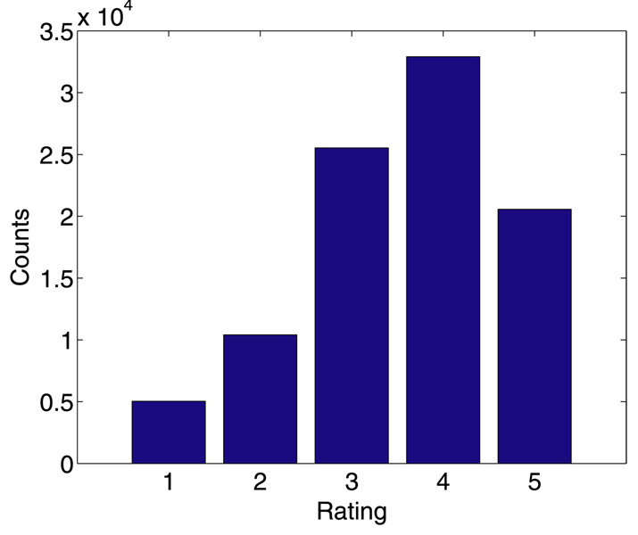
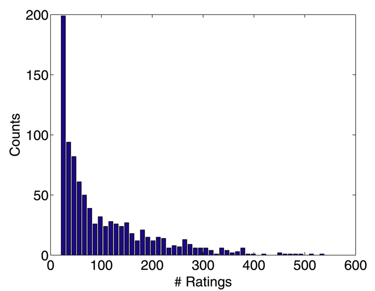
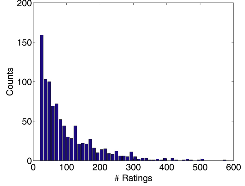
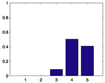
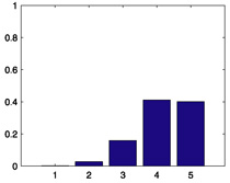
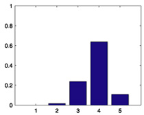
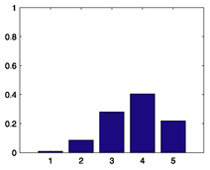
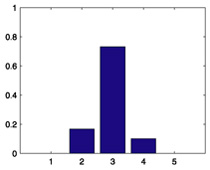
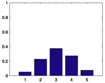
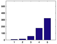
We start with some summary statistics. The 94,443 movie ratings have mean 3.57, variance 1.22, and histogram displayed in Figure 1. The number of ratings per person ranges from 20 to 539, with mean 102.99, median 65, and histogram displayed in Figure 2. The number of ratings per movie ranges from 20 to 579, with mean 100.79, median 69, and histogram displayed in Figure 3. Star Wars (1977) receives the most ratings (579). Histograms for the randomly chosen raters 408, 565, 727, and 754 appear in the second column of Table 2 in Section 6. Histograms for the randomly chosen movies 166, 381, 692, and 864 appear in the second column of Table 3 in Section 6.

Figure 1.

Histogram of the 94,443 ratings.

Figure 2.

Histogram of the number of ratings each rater contributes.

Figure 3.

Histogram of the number of ratings each movie receives.

Table 2.

Raw and quirky-mode distributions for the sample raters.

Rater i	Histogram of xij, j ∈ Mi	Multinomial		Binomial
		π̂i	q(x|α̂i)	π̂i	q(x|α̂i)
408		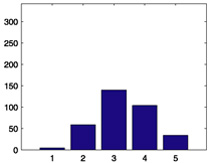0.3915		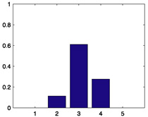0.3526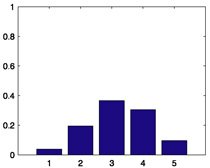
565		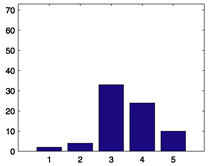0.3902		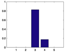0.4191
727		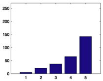0.3371		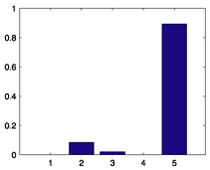0.2881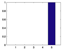
754		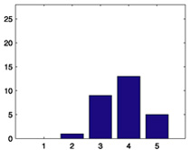0.6926		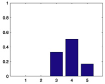0.7369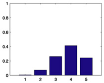

Table 3.

Raw and consensus-mode distributions for the sample movies.

Movie j	Histogram of xij	Multinomial c(x|β̂j)	Binomial c(x|β̂j)
166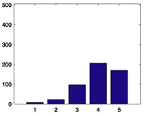
381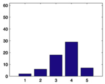
692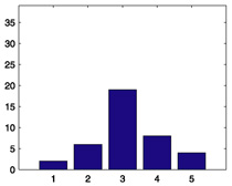
864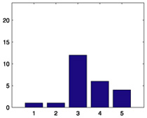

From the outset, it is worth emphasizing the transient popularity of most movies. Except for a few movies such as Casablanca, Schindler’s List, and Star Wars, it is doubtful that most of the highly rated movies from this period will survive the test of time.

3. AN ADMIXTURE MODEL

Suppose a website or company asks consumers to rate movies on an integer scale from 1 to d; often d = 5 or 10. Let M_i be the set of movies rated by person i. Denote the cardinality of M_i by |M_i|. Each rater does so in one of two modes that we will call “quirky” and “consensus.” In quirky mode, rater i has a private rating distribution with probability mass function q(x | α_i) that applies to every movie regardless of its intrinsic merit. In consensus mode, rater i rates movie j according to a distribution with probability mass function c(x | β_j) shared with all other raters in consensus mode. For every movie i rates, he or she makes a quirky decision with probability π_i and a consensus decision with probability 1 − π_i. These decisions are made independently across raters and movies. If x_ij is the rating given to movie j by rater i, then the likelihood of the data is

$$L(\theta )={\displaystyle \prod _i{\displaystyle \prod _{j\in M_i}[{\pi }_{i}q(x_{ij}|{\alpha }_i)+(1-{\pi }_i)c(x_{ij}|{\beta }_j)],}}$$ (1)

where θ = (π, α, β) is the parameter vector of the model. Once we estimate the parameters, we can rank the reliability of rater i by the estimate π̂_i and the popularity of movie j by its estimated average rating Σ_k kc(k | β̂_j) in consensus mode.

There are obviously many possibilities for the discrete densities q(x | α_i) and c(x | β_j). Probably the most natural choice is a multinomial distribution across the d categories. Under the multinomial model, the discrete densities are

$$q(k|{\alpha }_i)={\alpha }_{ik},c(k|{\beta }_j)={\beta }_{jk},k=1,\dots ,d.$$

Here the parameter vectors α_i = (α_i1, …, α_id) and β_j = (β_j1, …, β_jd) lie on the unit simplex in ℝ^d. We contrast this choice to the shifted binomial distribution with d − 1 trials and values 1, …, d rather than 0, …, d − 1. The discrete densities now become

$$\begin{array}{l}q(k|{\alpha }_i)=\left(\begin{array}{l}d-1\hfill \\ k-1\hfill \end{array}\right){\alpha }_i^{k-1}{(1-{\alpha }_i)}^{d-k},\hfill \\ c(k|{\beta }_j)=\left(\begin{array}{l}d-1\hfill \\ k-1\hfill \end{array}\right){\beta }_j^{k-1}{(1-{\beta }_j)}^{d-k},\hfill \end{array}$$

where the binomial parameters α_i and β_j occur on the unit interval [0,1]. The shifted binomial model is more parsimonious, but both models require a large number of parameters. If there are a raters and b movies, the multinomial model involves a + a(d − 1) + b(d − 1) free parameters. The shifted binomial model involves a + a + b free parameters. For the current dataset, these formulas translate into 8,333 and 2,771 free parameters, respectively. We will compare the fit of these two models by their AIC (Akaike information criterion) and BIC (Bayesian information criterion) numbers.

4. EM ALGORITHMS

Our natural impulse is to estimate parameters by the method of maximum likelihood. Although scoring and Newton’s method are not completely out of the question, they are apt to be frustrated by the large number of parameters and the constraints on the parameters. The advantage of Newton’s method is its quadratic rate of convergence. However, each iteration requires storage, calculation, and inversion of the observed or expected information matrix. These are expensive operations in high-dimensional problems. Also additional tactics are required to deal with parameter constraints and to keep the iterates from veering toward irrelevant stationary points. It is far easier to implement an EM algorithm (Dempster, Laird, and Rubin 1977; McLachlan and Krishnan 1997). We will compare the running times of both Newton’s method and the EM algorithm for the binomial model in Section 5.

The well-known EM algorithm for admixture models has been successfully applied in many settings (McLachlan and Peel 2000). To keep our exposition self-contained, we will derive the EM algorithm from the perspective of the more general MM algorithm (de Leeuw 1994; Heiser 1995; Becker, Yang, and Lange 1997; Lange, Hunter, and Yang 2000; Hunter and Lange 2004; Wu and Lange 2009). The MM algorithm, like the EM algorithm, is a principle for creating algorithms rather than a single algorithm. There are two versions of the MM principle. In maximization the acronym MM stands for iterative minorization-maximization; in minimization it stands for majorization-minimization. Here we deal only with the maximization version. Let f (θ) be the objective function we seek to maximize. An MM algorithm involves minorizing f (θ) by a surrogate function g(θ | θⁿ) anchored at the current iterate θⁿ of a search. Minorization is defined by the two properties

$$f({\theta }^n)=g({\theta }^n|{\theta }^n),$$ (2)

$$f(\theta )\ge g(\theta |{\theta }^n),\theta \ne {\theta }^n.$$ (3)

In other words, the surface θ ↦ g(θ | θⁿ) lies below the surface θ ↦ f (θ) and is tangent to it at the point θ = θⁿ. Construction of the minorizing function g(θ | θⁿ) constitutes the first M of the MM algorithm.

In the second M of the algorithm, we maximize the surrogate g(θ | θⁿ) rather than f (θ). If θⁿ⁺¹ denotes the maximum point of g(θ | θⁿ), then this action forces the ascent property f (θⁿ⁺¹) ≥ f (θⁿ). The straightforward proof

$$f({\theta }^{n+1})\ge g({\theta }^{n+1}|{\theta }^n)\ge g({\theta }^n|{\theta }^n)=f({\theta }^n)$$

reflects definitions (2) and (3) and the choice of θⁿ⁺¹. The ascent property is the source of the MM algorithm’s numerical stability. Strictly speaking, it depends only on increasing g(θ | θⁿ), not on maximizing g(θ | θⁿ).

One of the strengths of the MM principle is that we are allowed to work piecemeal on a complicated objective function such as the log of the likelihood (1). The art in devising an MM algorithm revolves around intelligent choices of minorizing functions and skill with inequalities. For our purposes, the crucial observation is that γ ↦ ln γ is a concave function. Therefore, Jensen’s inequality implies

$$\text{ln}\left({\displaystyle \sum _{i=1}^m{\gamma }_i}\right)\ge {\displaystyle \sum _{i=1}^m\frac{{\gamma }_i^n}{{\displaystyle {\sum }_{j=1}^m{\gamma }_j^n}}\text{ln}\left(\frac{{\displaystyle {\sum }_{j=1}^m{\gamma }_j^n}}{{\gamma }_i^n}{\gamma }_i\right).}$$ (4)

Note here that all parameter values are positive and that equality holds when ${\gamma }_i={\gamma }_i^n$ for all i.

If we apply the minorization (4) to a typical summand of the log-likelihood, then we get

$$\begin{array}{l}\text{ln}[{\pi }_{i}q(x_{ij}|{\alpha }_i)+(1-{\pi }_i)c(x_{ij}|{\beta }_j)]\ge w_{ij}^n\text{ln}\left[\frac{{\pi }_{i}q(x_{ij}|{\alpha }_i)}{w_{ij}^n}\right]+(1-w_{ij}^n)\text{ln}\left[\frac{(1-{\pi }_i)c(x_{ij}|{\beta }_j)}{1-w_{ij}^n}\right]\hfill \\ =w_{ij}^n\text{ln}{\pi }_i+(1-w_{ij}^n)\text{ln}(1-{\pi }_i)+w_{ij}^n\text{ln}q(x_{ij}|{\alpha }_i)+(1-w_{ij}^n)\text{ln}c(x_{ij}|{\beta }_j)+c_{ij}^n,\hfill \end{array}$$

where $c_{ij}^n$ is a constant that depends on θⁿ but not on θ and $w_{ij}^n$ is the weight

$$w_{ij}^n=\frac{{\pi }_i^{n}q(x_{ij}|{\alpha }_i^n)}{{\pi }_i^{n}q(x_{ij}|{\alpha }_i^n)+(1-{\pi }_i^n)c(x_{ij}|{\beta }_j^n)}.$$ (5)

This gives the overall surrogate

$$\text{ln}L(\theta )\ge {\displaystyle \sum _i\left[\text{ln}{\pi }_i{\displaystyle \sum _{j\in M_i}{w}_{ij}^n+\text{ln}(1-{\pi }_i){\displaystyle \sum _{j\in M_i}(1-w_{ij}^n)}}\right]}+{\displaystyle \sum _i{\displaystyle \sum _{j\in M_i}{w}_{ij}^n\text{ln}q(x_{ij}|{\alpha }_i)}}+{\displaystyle \sum _i{\displaystyle \sum _{j\in M_i}(1-w_{ij}^n)\text{ln}c(x_{ij}|{\beta }_j)}}+{\displaystyle \sum _i{\displaystyle \sum _{j\in M_i}{c}_{ij}^n.}}$$ (6)

The most remarkable feature of the surrogate is that it separates the parameters into convenient subsets for the maximization stage of the MM algorithm.

To estimate π_i, we treat ${\displaystyle {\sum }_{j\in M_i}{w}_{ij}^n}$ as the number of successes and ${\displaystyle {\sum }_{j\in M_i}(1-w_{ij}^n)}$ as the number of failures in |M_i| Bernoulli trials. Standard calculus arguments then yield the MM update

$${\pi }_i^{n+1}=\frac{1}{\left|M_i\right|}{\displaystyle \sum _{j\in M_i}{w}_{ij}^n.}$$

The updates of α and β depend on the model selected for the discrete densities q(x | α_i) and c(x | β_j).

Consider first the multinomial model. The surrogate function (6) cleanly isolates the contribution

$${\displaystyle \sum _{j\in M_i}{w}_{ij}^n\text{ln}q(x_{ij}|{\alpha }_i)={\displaystyle \sum _k{\displaystyle \sum _{j\in M_i}{1}_{\{x_{ij}=k\}}{w}_{ij}^n\text{ln}{\alpha }_{ik}}}}$$

of the quirky mode distribution α_i = (α_i1, …, α_id) for rater i. This is just the log-likelihood of a multinomial distribution with a noninteger count ${\displaystyle {\sum }_{j\in M_i}{1}_{\{x_{ij}=k\}}{w}_{ij}^n}$ for each proportion α_ik. Hence, the usual calculus argument with a Lagrange multiplier yields the MM update

$${\alpha }_{ik}^{n+1}=\frac{{\displaystyle {\sum }_{j\in M_i}{1}_{\{x_{ij}=k\}}{w}_{ij}^n}}{{\displaystyle {\sum }_{j\in M_i}{w}_{ij}^n}}.$$ (7)

Likewise, the surrogate function (6) isolates the contribution

$${\displaystyle \sum _i(1-w_{ij}^n)\text{ln}c(x_{ij}|{\beta }_j)={\displaystyle \sum _k{\displaystyle \sum _i{1}_{\{x_{ij}=k\}}(1-w_{ij}^n)\text{ln}{\beta }_{jk}}}}$$

of the consensus mode distribution β_j = (β_j1,…,β_jd) for movie j. By the same reasoning, we arrive at the MM update

$${\beta }_{jk}^{n+1}=\frac{{\displaystyle {\sum }_i{1}_{\{x_{ij}=k\}}(1-w_{ij}^n)}}{{\displaystyle {\sum }_i(1-w_{ij}^n)}}.$$ (8)

Under the binomial model, the parameters α_i and β_j are scalar success probabilities. There are d − 1 trials per observation, with the number of successes x_ij − 1 ranging from 0 to d − 1. Because the surrogate function separates the parameters, we get the MM updates

$${\alpha }_i^{n+1}=\frac{{\displaystyle {\sum }_{j\in M_i}{w}_{ij}^n(x_{ij}-1)}}{(d-1){\displaystyle {\sum }_{j\in M_i}{w}_{ij}^n}},$$ (9)

$${\beta }_j^{n+1}=\frac{{\displaystyle {\sum }_i(1-w_{ij}^n)(x_{ij}-1)}}{(d-1){\displaystyle {\sum }_i(1-w_{ij}^n)}}.$$ (10)

These updates make intuitive sense. The average number of successes per rater or movie is equated to the ratio of the total conditional number of successes to the total conditional number of trials.

For both the multinomial and binomial models, the MM algorithms coincide with their EM counterparts. In the EM setting the missing data consist of indicator random variables assigning each person-movie pair (i, j) to quirky or consensus mode. The weights $w_{ij}^n$ are the conditional expectations of the missing indicators calculated by Bayes’s rule; the Q function of the EM algorithms reduces to the surrogate function (6). One advantage of the MM principle is its generality. For example, if we model the q(x | α) and c(x | β) by beta-binomial distributions, then maximization of the Q function in the EM algorithm has to be done numerically. In contrast it is straightforward to invoke further minorizations and derive an explicit MM algorithm (Zhou and Lange 2009).

5. IMPLEMENTATION OF THE TWO MODELS

We implemented the two MM algorithms in Matlab. As demonstrated earlier, both algorithms enjoy the ascent property. In applying the algorithms, we iterate until the relative change of the log-likelihood between successive iterations falls below a preset threshold. In other words, we stop at iteration n when

$$\frac{|\text{ln}L({\theta }^n)-\text{ln}L({\theta }^{n-1})|}{|\text{ln}L({\theta }^{n-1})|+1}<\epsilon$$

for a small ε > 0. In the multinomial model, we start with the neutral values ${\pi }_i^0=\frac{1}{2},{\alpha }_{ik}^0=\frac{1}{d}$, and ${\beta }_{jk}^0=\frac{1}{d}$. For the binomial model, we start with the neutral values ${\pi }_i^0=\frac{1}{2},{\alpha }_i^0=\frac{1}{2}$, and ${\beta }_j^0=\frac{1}{2}$. Table 1 records the results of running the two algorithms on the MovieLens data on a laptop computer. In the table we adopt the convergence criterion ε = 10⁻⁹. If we adopt the looser criterion ε = 10⁻⁴, the multinomial algorithm converges in just 22 iterations and the binomial model in 27 iterations. For a simple comparison, we also fit the binomial model using the fmincon function (Trust–Region–Reflective Algorithm) in the Matlab optimization toolbox. This interior-reflective Newton’s method takes 2,391 iterations and 1,068 seconds to achieve the same log-likelihood.

Table 1.

Comparison of the two admixture models.

Model	ln L(θ̂)	# parameters	AIC	BIC	Iterations	Time secs
Multinomial	−112,529	8,333	241,724	320,519	423	169
Binomial	−119,085	2,771	243,712	269,914	673	194

In terms of model selection, it is interesting that the AIC favors the multinomial model whereas the BIC favors the binomial model. On data with a finer rating scale such as the IMDB data with d = 10, we imagine that the AIC would also favor the more parsimonious binomial model. A simple likelihood ratio test does not apply here because the maximum likelihood estimates of many parameters fall on a boundary and invalidate the chi-square approximation.

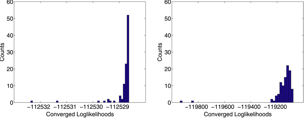
As mentioned, the models suffer from multiple likelihood modes. To assess the magnitude of the problem, we restarted the likelihood search in each model from 100 random points. For both models we sampled the π_i independently and uniformly from the interval [0, 1]. In the binomial model, we sampled the scalar success probabilities α_i and β_j similarly. In the multinomial model, we sampled the proportion vectors α_i and β_j independently and uniformly from the unit simplex in ℝ⁵. Figure 4 shows the histograms of the converged log-likelihoods under the stopping criterion ε = 10⁻⁹. For the binomial model, the log-likelihoods range from −119,937.5 to −119,076.8; for the multinomial model, the log-likelihoods range from −112,532.4 to −112,528.6. The binomial model exhibits more severe multimodality problems. Fortunately, in both models the neutral starting points lead to converged log-likelihoods within 0.01% of the best log-likelihoods found. For the sake of reproducibility, all subsequent results are based on the estimates from the neutral starting points under the stopping criterion ε = 10⁻⁹.

Figure 4.

Local maxima from 100 random starting points. Left: Multinomial model. Right: Binomial model.

6. MORE DETAILED RESULTS

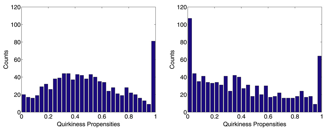
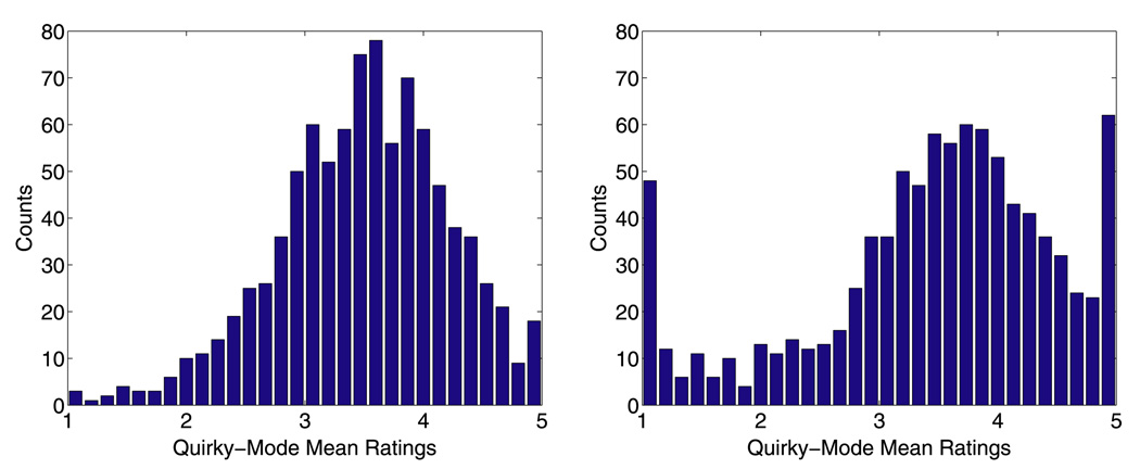
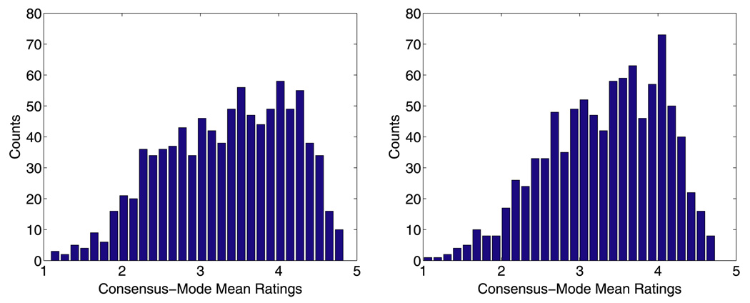
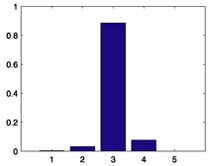
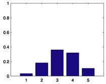
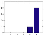
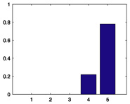
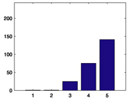
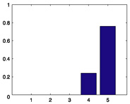
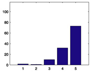
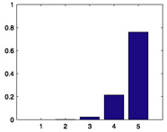
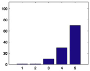
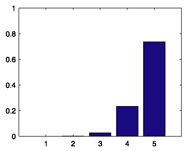
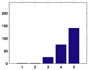
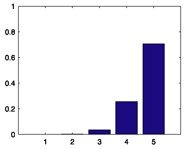
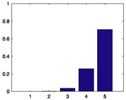
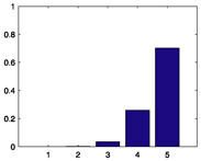
The differences between the two models are strikingly obvious when we examine the estimated propensities π̂_i for rating in quirky mode. Figure 5 displays histograms of these estimates under the two models. For a sizeable proportion of raters, π̂_i is approximately 1, particularly under the multinomial model. The binomial model identifies more raters at the other extreme when π̂_i is approximately 0 and a rater acts completely in consensus mode. Figure 6 plots the histograms of the means of the estimated quirky mode distributions q(x | α̂_i) for both models. The binomial model suggests that quirky raters tend to be more polarized in their ratings. Figure 7 plots the corresponding histograms for the consensus mode distributions. A glance at these plots shows that the two models differ more in how they handle quirky mode than in how they handle consensus mode. Tables 2 and 3 display histograms of the raw and estimated rating distributions for the four sample raters and the four sample movies. Tables 4 and 5 provide detailed estimates for the five top-ranked movies. Finally, Table 6 shows the top ten raw, multinomial, and binomial rankings.

Figure 5.

Histogram of the estimated quirkiness propensities π̂_i. Left: Multinomial model. Right: Binomial model.

Figure 6.

Histogram of the means of the estimated quirky-mode rating distributions. Left: Multinomial model. Right: Binomial model.

Figure 7.

Histogram of the means of the estimated consensus-mode rating distributions. Left: Multinomial model. Right: Binomial model.

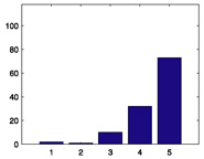
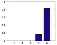
Table 4.

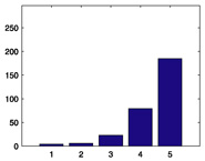
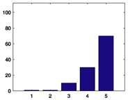
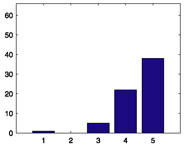
Top five movies under the multinomial model.

Rank	Title	Genre	Mean	# ratings	Histogram of xij	Consensus-mode distribution c(x|β̂j)	Bootstrap confidence
1	The Wrong Trousers (1993)	Animation	4.8356	118			36%
2	Schindler’s List (1993)	Drama, war	4.8054	297			25%
3	A Close Shave (1995)	Animation	4.7823	112			33%
4	Wallace & Gromit: The Best of Aardman Animation (1996)	Animation	4.7805	66			53%
5	Casablanca (1942)	Drama, war, romance	4.7605	243			32%

Table 5.

Top five movies under the binomial model.

Rank	Title	Genre	Mean	# ratings	Histogram of xij	Consensus-mode distribution c(x|β̂j)	Bootstrap confidence
1	The Wrong Trousers (1993)	Animation	4.7362	118			17%
2	A Close Shave (1995)	Animation	4.7070	112			17%
3	Casablanca (1942)	Drama, war, romance	4.6679	243			6%
4	Star Wars (1977)	Sci-Fi	4.6650	579			22%
5	Wallace & Gromit: The Best of Aardman Animation (1996)	Animation	4.6630	66			31%

Table 6.

Top ten movies.

Rank	Raw	Multinomial	Binomial	Male	Female	Age ≤ 30	Age > 30
1	A Close Shave (1995)	The Wrong Trousers (1993)	The WrongTrousers (1993)	Casablanca (1942)	The Wrong Trousers (1993)	The Umbrellas of Cherbourg (1964)	Shall We Dance? (1996)
2	The Wrong Trousers (1993)	Schindler’s List (1993)	A Close Shave (1995)	Citizen Kane (1941)	Shall We Dance? (1996)	Paths of Glory (1957)	Schindler’s List (1993)
3	Schindler’s List (1993)	A Close Shave (1995)	Casablanca (1942)	A Close Shave (1995)	Persuasion (1995)	The Wrong Trousers (1993)	Casablanca (1942)
4	Casablanca (1942)	Wallace & Gromit: The Best of Aardman Animation (1996)	Star Wars (1977)	The Wrong Trousers (1993)	Ma vie en rose (1997)	The Shawshank Redemption (1994)	The Wrong Trousers (1993)
5	Wallace & Gromit: The Best of Aardman Animation (1996)	Casablanca (1942)	Wallace & Gromit: The Best of Aardman Animation (1996)	Star Wars (1977)	Turbulence (1997)	A Close Shave (1995)	Some Folks Call It a Sling Blade (1993)
6	The Shawshank Redemption (1994)	Star Wars (1977)	Shall We Dance? (1996)	Schindler’s List (1993)	Once Were Warriors (1994)	Wallace & Gromit: The Best of Aardman Animation (1996)	Wallace & Gromit: The Best of Aardman Animation (1996)
7	Rear Window (1954)	The Shawshank Redemption (1994)	Schindler’s List (1993)	The Godfather (1972)	Paradise Lost: The Child Murders at Robin Hood Hills (1996)	Star Wars (1977)	A Close Shave (1995)
8	The Usual Suspects (1995)	Citizen Kane (1941)	The Shawshank Redemption (1994)	Wallace & Gromit: The Best of Aardman Animation (1996)	A Close Shave (1995)	Titanic (1997)	The Usual Suspects (1995)
9	Star Wars (1977)	The Godfather (1972)	The Usual Suspects (1995)	The Usual Suspects (1995)	Wallace & Gromit: The Best of Aardman Animation (1996)	The Godfather (1972)	Star Wars (1977)
10	12 Angry Men (1957)	The Usual Suspects (1995)	The Godfather (1972)	The Shawshank Redemption (1994)	Some Folks Call It a Sling Blade (1993)	The Manchurian Candidate (1962)	Citizen Kane (1941)

Although it is hard to draw absolutely convincing conclusions from this complex interplay of data and models, it seems safe to say that the raw rankings differ more from the two model rankings than the two model rankings differ from each other. We will address how to estimate the confidence of the rankings in a moment. Perhaps, a more interesting question is what happens to the rankings when we stratify raters by gender and age. Table 7 tallies the number of raters and ratings for four different subsets and lists their average estimated propensities π̂_i under both the multinomial and binomial models. Women and older people operate in quirky mode more often than men and younger people. In the case of females, this difference may stem from the fact that 70% of the raters are male.

Table 7.

Average propensities π̂_i for different subsets of the raters.

Subset	Number of raters	Number of ratings	Multinomial average π̂i	Binomial average π̂i
Whole	917	94,443	0.5040	0.4102
Female	261	23,905	0.5589	0.4550
Male	656	70,538	0.4821	0.3924
≤30	439	48,592	0.4957	0.3946
>30	478	45,851	0.5116	0.4246

The last four columns of Table 6 contain the top 10 ranked movies for each of the subsets under the multinomial model. It is worth noting that the high female rankings of the movies Ma vie en rose, Turbulence, Once Were Warriors, and Paradise Lost: The Child Murders at Robin Hood Hills may reflect the low number of ratings these movies receive (9, 2, 7, and 7, respectively). Similarly, the high rankings of The Umbrellas of Cherbourg and Paths of Glory by people under 30 may be artifacts of the low number of ratings these movies receive (1 and 10, respectively). Some of the intergroup differences are predictable. Females liked Persuasion and Shall We Dance, and males liked Casablanca and Star Wars. People under 30 liked Titanic, and people over 30 liked Schindler’s List.

7. CONFIDENCE IN RANKINGS

An obvious question is should we trust the rankings of movies or the credibility of the raters implied by the model estimates? If a movie is rated just a handful of times, then its estimated consensus distribution is apt to be highly variable and may not adequately reflect the true popularity or reputation of the movie. This pitfall may be avoided in at least three ways. First, as in our sample dataset, we may drop movies with low numbers of ratings. Second, in principle we may calculate the asymptotic standard error of the rank statistic Σ_k kc(k|β̂_j) for each movie j. Third, we can estimate the distribution of the rankings by the bootstrap. We briefly explore the bootstrap option here.

The bootstrap is a computationally intensive procedure for estimating the sampling distribution of a statistic. In our setting, suppose the data consist of r ratings. Consider the original data as an r × 3 matrix in which each row is of the form (raterID, movieID, rating). Then in each bootstrap replica, we resample the rows r times with replacement. The EM algorithm is performed on the bootstrap sample, and the rankings are recorded. This procedure is performed a large number of times. The reliability of an observed ranking can be estimated by the fraction of the time the same or a higher ranking appears in the bootstrap samples. Note that in principle a specific movie may not appear in some bootstrap samples. Also in a bootstrap sample a rater may rate the same movie several times. In the latter case, we assume that each of the repeated ratings is independent. We performed B = 100 bootstrap replicas on the MovieLens dataset. The last column of Tables 4 and 5 shows the bootstrap confidence values for the rankings. For example, under the multinomial model, the movie The Wrong Trousers is top ranked in 36 of the 100 bootstrap replicas; the movie Schindler’s List is in the top 2 movies in 25 of the 100 bootstrap replicas, and so on.

8. DISCUSSION

It is in the interest of commercial entities such as Netflix to predict customers’ future movie ratings. This translates into a classical prediction problem. Given the maximum likelihood estimates for either the multinomial or binomial models, it is natural to assume that rater i will rate movie j according to the distribution π̂_iq(x | α̂_i) + (1 − π̂_i)c(x | β̂_j). Hence, the estimated mean x̂_ij = π̂_i Σ_k kq(k | α̂_i) + (1 − π̂_i) Σ_k kc(k | β̂_j) is a sensible predictor of how customer i will rank movie j. If an integer ranking is desired, then the mode of the distribution π̂_iq(x | α̂_i) + (1 − π̂_i)c(x | β̂_j) might serve better.

The models explored here should be considered preliminary. They can be elaborated in simple ways. For instance, we could replace the binomial distribution throughout by the beta-binomial. As previously noted, the MM algorithms successfully generalize. Alternatively, one could use a mixed model with binomial quirky distributions and multinomial consensus distributions, or vice versa. In any event, good models in this field will have to reach a balance between detail and computability. Datasets are large and getting larger. Overelaborate models tend to be intractable. In this context we would like to raise the following challenges: (a) how can we integrate important covariates such as gender and age into the estimation process, (b) how can we incorporate correlations in intraperson ratings, and (c) how can we exploit people with similar rankings but shifted ratings? These are the million dollar questions in our thinking, not the short-term questions raised by the Net-flix contest. Because ranking extends far beyond movies, we should sort out the differences between explicit models and machine learning techniques. The future of statistics hinges on which is the better approach across a spectrum of problems.

REFERENCES

- ACM SIGCHI. RecSys’07: Proceedings of the 2007 ACM Conference on Recommender Systems. Minneapolis, MN: 2007. [Google Scholar]
- ACM SIGKDD and Netflix. Proceedings of KDD Cup and Workshop. 2007 available at http://www.cs.uic.edu/liub/Netflix-KDD-Cup-2007.html. [Google Scholar]
- Adomavicius G, Tuzhilin A. Toward the Next Generation of Recommender Systems: A Survey of the State-of-the-Art and Possible Extensions. IEEE Transactions on Knowledge and Data Engineering. 2005;17:734–749. [Google Scholar]
- Becker MP, Yang I, Lange K. EM Algorithms Without Missing Data. Statistical Methods in Medical Research. 1997;6:37–53. doi: 10.1177/096228029700600104. [DOI] [PubMed] [Google Scholar]
- de Leeuw J. Block Relaxation Algorithms in Statistics. In: Bock HH, Lenski W, Richter MM, editors. Information Systems and Data Analysis. New York: Springer-Verlag; 1994. pp. 308–325. [Google Scholar]
- Dempster AP, Laird NM, Rubin DB. Maximum Likelihood From Incomplete Data via the EM Algorithm. Journal of the Royal Statistical Society, Ser. B. 1977;39:1–38. (with discussion) [Google Scholar]
- Heiser WJ. Convergent Computing by Iterative Majorization: Theory and Applications in Multidimensional Data Analysis. In: Krzanowski WJ, editor. Recent Advances in Descriptive Multivariate Analysis. Oxford: Clarendon Press; 1995. pp. 157–189. [Google Scholar]
- Hunter DR, Lange K. A Tutorial on MM Algorithms. The American Statistician. 2004;58:30–37. [Google Scholar]
- Lange K, Hunter DR, Yang I. Optimization Transfer Using Surrogate Objective Functions. Journal of Computational Statistics. 2000;9:1–59. [Google Scholar]
- McLachlan GJ, Krishnan T. The EM Algorithm and Extensions. New York: Wiley; 1997. [Google Scholar]
- McLachlan GJ, Peel D. Finite Mixture Models. New York: Wiley; 2000. [Google Scholar]
- Wu TT, Lange K. The MM Alternative to EM. Statistical Science. 2009 to appear. [Google Scholar]
- Zhou H, Lange K. MM Algorithms for Some Discrete Multivariate Distributions. 2009 doi: 10.1198/jcgs.2010.09014. to appear. [DOI] [PMC free article] [PubMed] [Google Scholar]