Dynamics of Choice: A Tutorial

Abstract

Choice may be defined as the allocation of behavior among activities. Since all activities take up time, choice is conveniently thought of as the allocation of time among activities, even if activities like pecking are most easily measured by counting. Since dynamics refers to change through time, the dynamics of choice refers to change of allocation through time. In the dynamics of choice, as in other dynamical systems that include feedback, change is away from perturbation and toward a steady state. Steady state or equilibrium is assessed on a longer time scale than change because change is only visible on a smaller time scale. When we compare laws of equilibrium, such as the matching law with laws of dynamics, two possibilities emerge. Self-similarity occurs when the same law can be seen across smaller time scales, with the result that the law at longer time scales may be understood as the expression of its application at smaller time scales. Reduction occurs when the dynamics at a small time scale are incommensurate with the dynamics at longer time scales. Then the process at the longer time scale is reduced to a qualitatively different process at the smaller time scale, as when choice is reduced to switching patterns. When reduction occurs, the dynamics at the longer time scale may be derived from the process at the smaller time scale, but not the other way around. Research at different time scales is facilitated by the molar view of behavior.

This tutorial addresses the dynamics of choice in the framework of the molar view of behavior (Baum, 2002; 2004). It considers choice to constitute allocation of behavior among activities and to occur on multiple time scales. It describes basic principles and gives examples.

Choice As Allocation

What is choice? In everyday talk, people speak of “choices” or “making a choice” as if choice were a momentary event. However, when someone says, “I made up my mind to take the job,” he or she is referring to a switch from one pattern of life activities to another. Even when someone chooses to buy one dress rather than another, the small-scale event referred to is a switch from a life without wearing that dress to one in which the dress is sometimes worn. Thus, talking about choice this everyday way only focuses on switching activities, which is a view on an extremely small time scale, as we shall see later.

To be alive is to behave. By definition, behavior is assigned to a living, whole organism (Rachlin, 1994). In 24 hours of observation, one measures 24 hours' worth of behavior. The most fundamental property of behavior is that it takes up time.

Choice in the present context consists of the allocation of time among two or more activities. In two earlier papers, I argued that all behavior is choice, because every situation permits more than one activity (Baum, 2002; 2004). One cannot create, even in the laboratory, a situation so impoverished that the organism can engage in only one activity. Pigeons and rats, for example, bring to experimental chambers their own species-specific and individual-specific activities—often referred to as “background activities” in contrast with measured operant activity. I argued also that all behavior entails choice too, because every activity has parts that are themselves activities. Thus, a rat's interactions with the response levers in an experiment may entail pressing on the left lever and pressing on the right lever. Either of these activities, in turn, entails parts such as licking, biting, and pawing the lever (Baum, 1976). If behavior is choice and also entails choice, then to speak of choice is to speak of behavior, and to speak of behavior is to speak of choice. Thus, the dynamics of choice is the dynamics of behavior.

When we examine the parts of an activity, we consider activities that occur on a smaller time scale than the activity to which they belong. Manifesting a preference between two response keys takes longer than pecking at either one of them; loving another person takes longer than kissing that person. We shall consider time scale in relation to dynamics later.

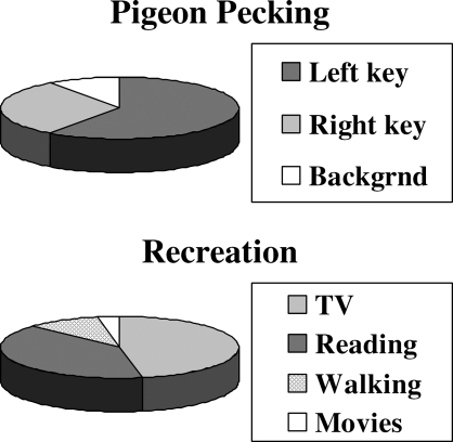
Figure 1 illustrates the idea of allocation. These charts compare allocation to cutting up a pie. They express the understanding that time is finite—that is, in an hour's observation time, one records an hour of behavior; in the course of a year, a person engages in a year's worth of behavior. The chart on the top illustrates time spent in a hypothetical experiment in which a pigeon pecks at two response keys; much time is spent pecking at the left key, some time is spent pecking at the right key, and some time is spent in background activities. The chart on the bottom shows a hypothetical person's allocation of recreational time among some recreational activities. The most time is spent watching TV, a large amount of time is spent reading for pleasure, some time is spent taking walks, and a small amount of time is spent watching movies.

Fig 1.

Hypothetical examples illustrating the concept of allocation. Choice is the allocation of time among activities.

If conditions change, we expect that allocation will change. If the schedule of earning food changes, and now the right key provides more, the allocation of pecking between left key and right key will change to favor the right key. If the person forms a relationship with someone who loves movies, the time allocated to watching movies will increase, and either of two changes will occur. If recreational time remains fixed, the time spent in some other recreational activity will decrease. If recreational time expands, the time spent in some activity that competes with recreation will decrease. The finiteness of time means that when one activity increases others must decrease. In an applied setting, such as a classroom, if an intervention increases a child's time on task, it must also decrease other activities, such as yelling and hitting other children.

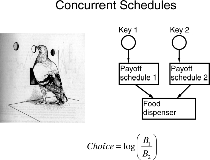
For purposes of illustration, the situations I shall take up will all be ones in which a pigeon pecks at two response keys and occasionally receives access to food by pecking one or the other key. Figure 2 diagrams the arrangement. Each key is associated with a payoff schedule and operates the food dispenser, making it briefly available, according to that schedule. In all the examples I will take up, the two payoff schedules will be variable-interval schedules, on which food is made available at unpredictable times. The measure of choice or allocation will be the logarithm of the ratio of pecks at one key (e.g., the left key) to pecks at the other (e.g., the right key). Pecks are counted as a surrogate for time out of convenience; the number of times a pigeon's activity with respect to a key operates a microswitch attached to the key is a good indication of the time spent in that activity.

Fig 2.

A typical experimental arrangement for studying and measuring choice. Drawing reprinted with the author's permission from Hall (1983), page 43.

Dynamics as Change

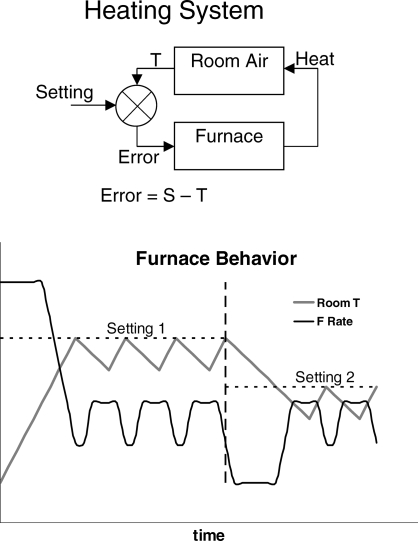
Dynamics may be contrasted with stability—change versus equilibrium. Since dynamics refers to change through time, dynamics of choice refers to change of allocation through time. We expect to see dynamics whenever conditions in a situation change and behavior shifts from a previous steady state to approach a new steady state. Such a pattern of dynamics followed by equilibrium implies a feedback system. By way of illustration, the upper diagram of Figure 3 shows a diagram of a heating system. The thermostat compares the temperature of the room air T with the setting S. If the error S-T is greater than zero, the furnace turns on. Its output is heat, which increases the temperature of the room air, until the error decreases to zero, and the furnace turns off. As long as the error remains zero, no action occurs, but as soon as the system is perturbed by, say opening a window or changing the setting, action begins again; the furnace turns on. The lower diagram in Figure 3 illustrates the dynamics of the system. At the extreme left, the thermostat setting is increased to Setting 1, with the result that the furnace is at a high level of activity. Room temperature increases until it reaches Setting 1, whereupon the activity of the furnace decreases. Since no room is perfectly insulated, room temperature gradually falls. The furnace increases its activity in response, and a repeating cycle occurs, in which temperature falls and increases as the furnace cycles between low and higher activity. This cycle continues indefinitely and constitutes the system's equilibrium state. At the broken vertical line, the setting of the thermostat is reduced to Setting 2. The furnace activity decreases, and doesn't increase again until room temperature falls below the new setting, producing positive error. From that point onwards, the cycling of steady state returns, maintaining temperature near the setting.

Fig 3.

A heating system as an example of a feedback system. Top: diagram of the feedback system showing error controlling feedback. Bottom: the behavior of the system in response to changes in setting. The broken vertical line indicates a change in setting.

Three earlier papers likened the organism and its environment to a feedback system (Baum, 1973; 1981; 1989). Although many important events in the environment are outside the organism's control, some are affected by behavior. This dependency forms the basis for comparing the behavior and environment to a feedback system, and may be expressed in the concept of a feedback function—that is, a function determined by the environment that transfers behavior as input into valued events as output. In the laboratory, feedback functions are arranged by payoff schedules (Baum, 1973; 1981; 1989). Sometimes schedules mimic properties of the natural environment, such as a patchy resource obtained by foraging (Baum, 1989).

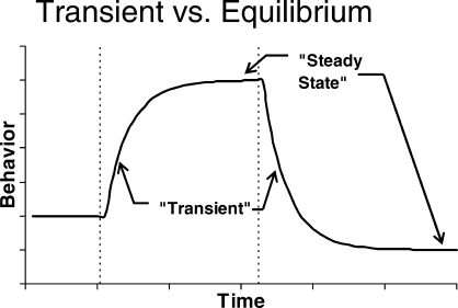
The action of a behavioral feedback system analogous to that in Figure 3 will resemble the pattern shown in Figure 4. Although “steady state” should include small-scale fluctuations like those shown in Figure 3, it is represented for simplicity in Figure 4 as a horizontal line. At the first broken vertical line, conditions are changed. The result is change in behavior during what is sometimes called the “transient” phase, as behavior approaches a new “steady state.” At the second vertical line, conditions are changed again, and again behavior passes through a transient phase as it approaches another steady state. Dynamics are revealed in these transient phases.

Fig 4.

The pattern of transient adjustment to equilibrium or steady state expected from a feedback system like that in Figure 3. Condition changes are indicated by broken vertical lines.

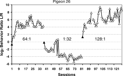
Real data are not so smooth. Figure 5 shows some examples from an experiment in which each pair of several pairs of VI schedules was maintained in effect for many daily sessions (Baum, Schwendiman, & Bell, 1999). The data were produced by an individual pigeon (B26). Each point shows the log (base 2) of the ratio of pecks at the left key to pecks at the right key calculated for one whole session. The first set of points shows allocation as behavior adjusted to a programmed 64∶1 food ratio after having stabilized on a 1∶9 food ratio. During the transient phase, allocation drives steadily toward stronger and stronger preference for the left key. Although variation from session to session never ceases, it eventually becomes unsystematic, and no trend is discernable as the pigeon's pecking consistently favors the left key. “Unsystematic” doesn't mean uncaused; various factors might contribute to the session-to-session variation, such as variation in the actual ratio of food deliveries for the session, just as imperfect insulation might cause variation in room temperature at equilibrium in Figure 3. After the last session of 64∶1, the food ratio was programmed to be 1∶32, and the allocation shifts accordingly, eventually again “stabilizing,” now at a level favoring the right key. Next, a 128∶1 food ratio is implemented, and behavior shifts through a transient phase to eventually strongly favor the left key.

Fig 5.

One pigeon's session-by-session choice in three conditions, each a different food ratio (Baum et al., 1999). Filled triangles indicate the first session of a new condition. The 64∶1 food ratio followed a 1∶9 food ratio.

Varieties of Procedure

The study of the dynamics of choice is a relatively recent development. One of the first studies that might be considered to address dynamics was by Davison and Hunter (1979). They exposed pigeons to various pairs of concurrent VI schedules, each for just six sessions. They found that preference grew and stabilized within the six sessions. Following up, Hunter and Davison (1985) and Schofield and Davison (1997) exposed pigeons to a pseudorandom binary sequence in which two pairs of VI schedules alternated randomly from session to session. On any day, a pigeon would get, for example, a 4∶1 food ratio or a 1∶4 food ratio, but unpredictably from day to day. They found that sessional preference was largely determined by the current food ratio and to a much smaller extent the previous session's food ratio. Some studies using a related procedure outside the purview of this article, concurrent-chain schedules, changed the schedules every day and measured rapid changes in preference both across and within sessions (e.g., Kyonka & Grace, 2008). Other research on concurrent VI schedules studied change of preference within sessions. Mazur (1992) found that when a 1∶1 food ratio was replaced with 2∶3, 3∶1, or 9∶1, preference shifted rapidly and started approaching equilibrium within a single session. Mark and Gallistel (1994), Gallistel, Mark, King, and Latham (2001), and Banna and Newland (2009) studied dynamics of choice following changes in food ratio within sessions. Davison and Baum (2000) adapted a procedure developed by Belke and Heyman (1994) to study the effects of changing randomly among seven food ratios within a session. In this experiment, pigeons pecked at two keys delivering food in one of the seven ratios until a certain number of food deliveries, ranging from 4 to 12, had occurred. Then a blackout occurred, and at the end of the blackout a new food ratio was presented. They found that preference developed rapidly even when food ratios lasted for only four food deliveries. Following each food delivery, preference shifted toward the key that had just produced the food, and a preference pulse occurred favoring that just-productive key. They studied the effects of a variety of parameters on preference in this rapidly changing environment (Baum & Davison, 2004; Davison & Baum, 2002, 2003, 2006, 2007). Aparicio and Baum (2006, 2009) studied similar procedures with rats.

Dynamics and Time Scale

Figure 5 illustrates an important difference between steady-state or equilibrium behavior and the dynamics seen in the transient phase. Estimating steady state would require several of the final sessions to average across the unsystematic variation, whereas viewing the dynamics requires looking session by session for the changing allocation to be visible. In practice, estimating steady state requires a relatively long time scale, whereas viewing the dynamics requires a shorter time scale. In Figure 5, the shorter time scale is based on the session as a unit, but when conditions change from session to session, steady state or the approach to it may occur within a session, and then the shorter time scale requires a smaller unit than the whole session. In procedures that present several components, each with a different food ratio, within each single session, approach to stability may occur on a still smaller time scale, and viewing the dynamics requires a still smaller unit, such as the interfood interval (e.g., Aparicio & Baum, 2009; Baum & Davison, 2004). Dynamics may occur even within the interfood interval, and then a unit smaller than that is required, such as the bout or visit to a key, a unit demarcated by a switch from one key to the other.

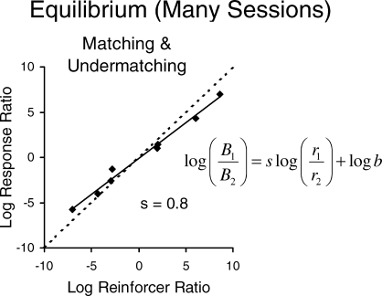
The longest time scale usually studied is steady state or equilibrium across many sessions, as shown in Figure 5. In that experiment, several food ratios besides those shown in Figure 5 were studied, and the relation between behavior ratio and food ratio at equilibrium appears in Figure 6. The broken line in Figure 6 represents the locus of perfect matching, in which the behavior ratio would be equal to the food ratio. The data points are fitted to the solid regression line, the equation of which is to the right. The line has a slope s of 0.8, falling short of matching, a common result called “undermatching” (Baum, 1974; 1979). Close inspection of Figure 5 reveals that the three steady states hover near the log (base 2) of the programmed food ratio—6.0 for 64∶1, −5.0 for 1∶32, and 7.0 for 128∶1—as one would expect from the matching relation.

Fig 6.

The matching relation across steady-state estimates of choice based on several sessions (Baum et al., 1999). The regression line shows the relation between log (base 2) behavior ratio (allocation) and log (base 2) food ratio. The slope of 0.8 shows undermatching.

Although the matching relation is a reliable finding, it doesn't necessarily tell us anything about dynamics, because it is a relation across many steady states, between which the dynamics are simply omitted. Whether the matching relation can be found in the dynamics as well as in equilibrium is a question requiring us to look at the behavior between the steady states. If we find the matching relation holds somehow in the dynamics, we could consider the matching relation to explain the results at equilibrium. If some other relation were to apply to the dynamics, however, then we would expect that relation to predict the matching at equilibrium, even though the matching at equilibrium doesn't apply to the dynamics. We will return to this point later when we discuss reduction.

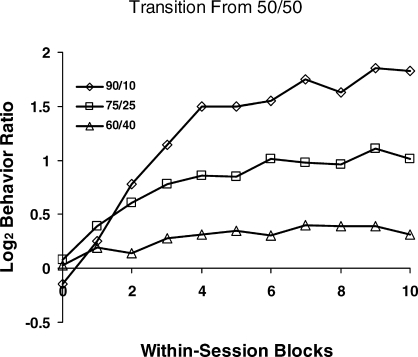
An example of dynamics that reflect the matching relation appears in some data gathered by Mazur (1992) using standard concurrent VI schedules (Figure 2). Figure 7 shows some of Mazur's results from a procedure in which steady state was achieved with a 1∶1 food ratio, and then the food ratio was abruptly switched to an unequal food ratio—60∶40, 75∶25, or 90∶10. (See Banna & Newland, 2009, for a recent similar experiment.) The lines show the dynamics within the first session of the new food ratio. Because the approach toward a new equilibrium occurs within the session, Mazur measured choice in smaller units of 9- or 15-min samples. Choice begins near indifference (zero), the prior steady state. Each curve resembles the approach to equilibrium idealized in Figure 4 and shown session by session in Figure 5, but on a smaller time scale than in Figure 5. Mazur didn't show the food ratios within the blocks, but since each curve rises toward a level that corresponds to the new food ratio, one may guess that choice was tracking the gradual approximation of food ratio delivered to the food ratio programmed. It falls short, however, for each condition, never reaching the level that would match the log food ratio—i.e., undermatching.

Fig 7.

Within-session dynamics in an experiment by Mazur (1992). The first point in each curve represents the final 15 min of performance on equal concurrent variable-interval schedules (50/50), and the curves show choice in 9- and 15-min blocks of the first session after a change in food ratio from 50/50 to 90/10, 75/25, or 60/40. Choice moves toward a new level appropriate to the new food ratio.

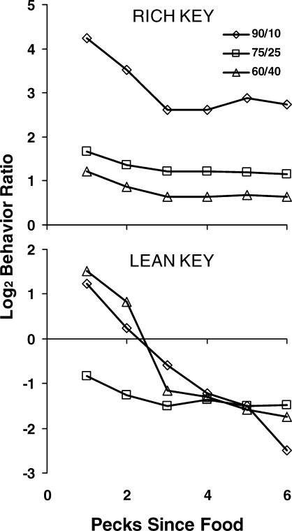
Another of Mazur's (1992) results appears in Figure 8, illustrating a still smaller time scale. In these graphs, choice is shown peck by peck for the first six pecks following a food delivery. Each graph is based on a sample of 500 pecks. Out of those pecks, some were the first to follow a food delivery, and Mazur calculated the percentage of those that operated the same key as produced the food. He did the same for second pecks following food, third pecks, and so on. In constructing Figure 8, I transformed Mazur's percentages to log ratios of pecks (just-productive key/not-just-productive key). Immediately following food from the rich key, choice strongly favored the just-productive key and then declined. Immediately following food from the lean key, choice weakly favored the just-productive key, but soon switched to favoring the rich key (negative log ratio). For the 75∶25 schedule, choice favored the rich key even immediately after food from the lean key. How these local shifts relate to the matching relation remains to be seen. Davison and I call such graphs “preference pulses” (Davison & Baum, 2000; 2003; 2006). More about preference pulses later.

Fig 8.

Choice on a smaller time scale in Mazur's (1992) experiment. The first point in each curve represents choice across all first pecks following food in a sample of 500 pecks. The second point represents choice across all second pecks, and so on. Choice is shown peck by peck for the lean alternative (lower graph) and the rich alternative (upper graph) in each of the three conditions of Figure 7 at the end of five sessions of exposure. Preference pulses are evident in the 90/10 condition, and only following food from the lean key in the 60/40 condition.

Self-Similarity versus Reduction

In the examples we have considered so far, all choice dynamics were examined at time scales that permitted calculation of a behavior ratio in each unit. If, as analysis moved to smaller and smaller time scales, one could still see the matching relation holding, one might be tempted to conclude that matching holds all the way down (e.g., Gallistel, King, Gottlieb, Balci, Papachristos, Szalecki, & Carbone, 2007). When the same relation applies at every time scale, that is self-similarity (also known as scale invariance). Suppose, however, that local (small-scale) processes do not reflect the extended regularity—that is, suppose the extended relation is not evident in the local processes. If such small-scale regularities exist, then matching might be derivable from them, but those small-scale regularities might not be derivable from the matching relation. For example, suppose that bouts of pecking at the two keys change in regular ways within the interfood interval. This would imply regular dynamics in switches from one key to the other. Although one would expect to be able to derive the matching relation from the switching, the opposite—deriving switching from matching—would fail. In other words, the dynamics of choice would be reduced to the bouts or switches in this example of what I will call reduction.

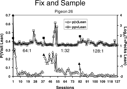
One may examine bouts or visits at the keys across sessions too. Figure 9 shows the same sessions as in Figure 5, but with a view to understanding switching between keys. The top graph shows a transform of the average number of pecks in a visit to the lean alternative (right-hand vertical axis). If the average visit is one peck, the measure equals 1.0. Across the three food ratios, the average visit is always longer in the first session of the new ratio (filled squares), when the ratio has just switched rich and lean keys. After several sessions, it approaches and sometimes equals one peck. The lower graph shows the probability of visiting the lean key calculated for each session (number of visits to the lean key divided by number of pecks at the rich key). It starts high, when the lean alternative was recently the rich alternative, but drops to a low level—lowest for 128∶1, higher for 64∶1, and highest for 32∶1. This pattern of fixing on the rich key and occasionally visiting the lean key, according to the food ratio, I call “fix and sample” (Aparicio & Baum, 2006; Baum et al., 1999; Baum & Davison, 2004).

Fig 9.

The same data from Baum et al. (1999) as in Figure 5 replotted to show session by session the average number of pecks in a visit to the lean key (squares; vertical axis on the right) and the probability of visiting the lean key (triangles; vertical axis on the left). Pecks per visit (vertical axis on the right) was transformed by adding one and taking the logarithm. Filled symbols show the first session of a new condition. The brief visits to the lean key and the graded probabilities of visiting the lean key are consistent with a fix-and-sample pattern of responding on the two keys.

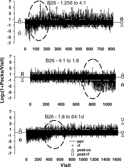
The dynamics of choice seen in the visits to the keys may be viewed also within the first session of a new food ratio. Figure 10 shows all visits in the first session of each of three conditions from the same experiment: the first session of 4∶1 food ratio following 1∶256, of 1∶8 following the previous 4∶1, and of 64∶1 following the previous 1∶8. Each graph shows one entire session. The vertical axis represents the same transform of visit length as in Figure 9, but with the added feature that it is positive for visits to the left key and negative for visits to the right key. Since the visits necessarily alternate, they are plotted visit by visit. Visits to the previously rich key are longer at first, but at some point during the session (circled), this changes fairly abruptly and the longer visits are to the now-rich key. The fix-and-sample pattern reverses.

Fig 10.

The first session of each of three conditions in the Baum et al. (1999) experiment shown visit by visit as the visits alternate between the left and right keys. The vertical axis represents the same transform of visit length as in Figure 9, except that visits to the right are represented as negative. The length of each vertical line shows the length of one visit. Small diamonds show food deliveries. Triangles and squares show transformed visit length in the final stable state of a condition; the ones on the left are for the preceding condition, and the ones on the right are for the new condition. The absence of any pecks following food from the lean key (zero-length visit) appears as a square on the horizontal axis. The dominance of one-peck visits to the lean key appears as a triangle at 1 or −1. Each graph shows one entire session. At the beginning of the session, the pattern of visits is appropriate to the prior condition, and at some point during the session (circled) the pattern switches to favoring the newly rich key; visits to the rich key become long, and visits to the lean key become brief.

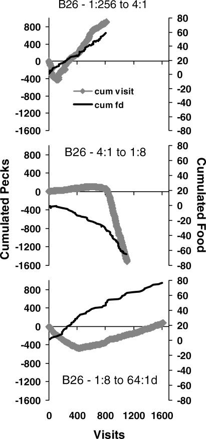
Figure 11 graphs the three sessions in a way that brings out the dynamics and the abruptness of the shift. The light line shows cumulated food deliveries (right-hand vertical axis), with a left food delivery counted as +1 and a right food delivery counted as −1. Each line starts at zero (vertical axis on the right) and slopes in the direction of the rich key. The heavy line shows cumulated pecks, with visits to the left counted as positive and visits to the right counted as negative. Choice favors the previously rich key at first, and then turns a corner to favor the presently rich key. Thus, the dynamics of choice appear in switching between keys within a session.

Fig 11.

The same data as in Figure 10 replotted to show the relatively abrupt transition in switching pattern. The lighter line shows cumulated food (vertical axis on the right) calculated by adding +1 for a food delivery from the left key and −1 for a food delivery from the right key. The line begins at zero, and the slope shows which was the richer alternative. The thicker line (diamonds) shows cumulated pecks calculated by adding the pecks in each visit to the left key and subtracting the pecks in each visit to the right key. In each session, cumulated pecks initially has a slope appropriate to the prior condition and then switches abruptly to a slope in the same direction as the cumulated food.

Frequent Transitions within Sessions: The Davison-Baum Procedure

Another approach to studying the dynamics of choice at various time scales is to arrange many transitions of food ratios within single sessions. In the procedure that Davison and I have studied, seven different food ratios are presented within a session, separated by blackouts, and with no signal as to the ratio in effect at the end of the blackout. Each component food ratio lasts for a number of food deliveries, usually 10 or 12, and then the blackout commences. We run many sessions like this, typically 65 to 100, and then use the last ones (50 to 85) in analysis. Thus, we study a performance that is stable session to session, but which reveals dynamics within the sessions. Across the many stable sessions, we gather large samples of events at time scales smaller than the session. That enables us to average across many instances of small-scale events.

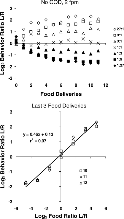
The upper graph in Figure 12 shows the dynamics of choice from food delivery to food delivery within the different components (Baum & Davison, 2004). The data were pooled across pigeons and for each component were pooled across all of its occurrences (i.e., one per session). The behavior ratio was calculated for pecks before any food (zero on the x axis), then for pecks occurring after the first and up to the second food delivery, then for pecks after the second and up to the third, and so on. In averaging this way, we treat the interfood interval as the scale unit. Choice begins near indifference, and then moves in the direction of the food ratio—except for the 1∶1 food ratio, for which choice appropriately stays near indifference. We see the approach toward equilibrium drawn in Figure 4, but on a smaller time scale than in Figure 5 or Mazur's (1992) within-session data in Figure 7, because the unit is the interfood interval. By the ninth food delivery, choice has separated across components, although the process may be incomplete or inherently limited, because the large ratios hardly differentiate at all; when the food ratio is 9∶1 or 27∶1, the rich key may deliver food 12 times in a row, making the ratios indistinguishable. Close inspection reveals that log (base 2) behavior ratio falls considerably short of log food ratio, indicating undermatching, as in Mazur's data (Figure 7). The lower graph in Figure 12 confirms this impression by showing the log behavior ratio versus the log food ratio for the last three food deliveries. Although the regression line fits the data well (r²  =  .97), the slope of the line (0.46) shows considerable undermatching.

Fig 12.

Within-component choice, calculated for each interfood interval, from one condition of the experiment reported by Baum and Davison (2004). Top: As more food deliveries occur, choice moves from indifference toward a level appropriate to the food ratio in the component. Bottom: Log behavior ratio (last three points in the upper graph) plotted against log obtained food ratio across the seven components. The regression line fits the points closely but shows considerable undermatching at the end of the components.

At this time scale, Davison and I developed a simple mathematical model to capture the changes in interfood choice following different left–right sequences of food deliveries (Baum & Davison, 2009). We used the equation

where B_i is log peck ratio (left/right) between the i^th and i+1^st food deliveries, A is the effect on choice of the i+1^st food delivery (positive for food produced by a peck at the left key; negative for food produced by a peck at the right key), and w is the weight of the present food in relation to present choice B_i in the averaging that predicts the next choice B_i+1. Updating predicted choice with Equation 1 food delivery by food delivery, we were able to account for over 90% of the variance in choice at this time scale.

Self-Similarity and Reduction at Small Time Scales

This same experiment provides us with examples of both self-similarity and reduction. Treating interfood intervals as whole units ignores dynamics that might occur between food deliveries. Preference pulses like those shown in Figure 8 allow us to examine dynamics within interfood intervals. The time scale is smaller; preference pulses may be revealed in small time bins (e.g., 1–3 s) following food delivery or, as in Figure 8, peck by peck, which implies the unit to be the time per peck. Either way, preference pulses are derived by averaging over many instances of food delivery—for example, in a sample of 80 sessions (560 components), one might find 280 instances of the first food delivery in a component coming from the left key.

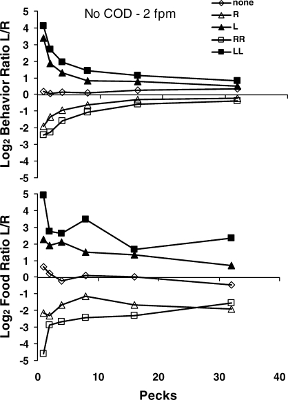
The upper graph in Figure 13 shows preference pulses following different food sequences at the beginning of a component: one food delivery from the left key (L); one food delivery from the right key (R); two in a row from the left key (LL); and two in a row from the right key (RR). As in Figure 8—Mazur's (1992) data—pecks appear on the horizontal axis as a surrogate for time. Instead of going peck by peck, however, the bins average across an increasing span of pecks: 1st pecks, then 2nd and 3rd pecks, then 4th to 7th, 8th to 15^th, 16^th to 31^st, and all beyond 32^nd. This was done to keep sample sizes large, because sample size necessarily decreases with time since food delivery, as fewer and fewer interfood intervals last long enough to provide data. In these curves, we again see the dynamic pattern of perturbation followed by movement toward equilibrium (Figure 4). At this time scale, the food itself constitutes the perturbing event. Immediately following food, choice strongly favored the just-productive key—the more so, if it produced two in a row. As time and pecks proceeded, however, choice dropped toward indifference. The points labeled “none” show choice from the beginning of the component before any food was delivered—no pulse occurred then, as we would expect if food delivery induces the pulse.

Fig 13.

Choice dynamics following food delivery in the Baum and Davison (2004) experiment. Top: Peck-by-peck choice following the beginning of the component (diamonds) and following one (triangles) or two (squares) food deliveries from the left key (filled symbols) or the right key (unfilled symbols). The first point represents all first pecks, the second point pecks 2 and 3, the third point pecks 4–7, the fourth point pecks 8–15, the fifth point pecks 16–31, and the last point all pecks beyond 32. Preference pulses appear following one or two food deliveries. Bottom: Log food ratio calculated from the occurrences of the next food following the beginning of the component (diamonds) or one or two food deliveries from the left or right key (same legend as the top graph). Food produced by each peck grouping on the horizontal axis was summed for the left and right keys and the ratio calculated. If food occurred again soon, it tended to be more often from the same key.

The lower graph in Figure 13 shows the food ratio, calculated from the source—left or right key—of the next food delivery. For example, if the first peck produced the next food, sometimes that peck produced food from the left key and sometimes from the right key, and the graph shows the log ratio of left food to right food. Similarly, if the second or third peck produced food, the second point shows the log ratio of left food to right food, and so on for all the peck bins. The graph shows that if the next food delivery occurred soon, it was likely from the same key as the one before—the more so, if that key had produced two in a row. If the next food delivery occurred later, however, it was less likely to be from the same key as before.

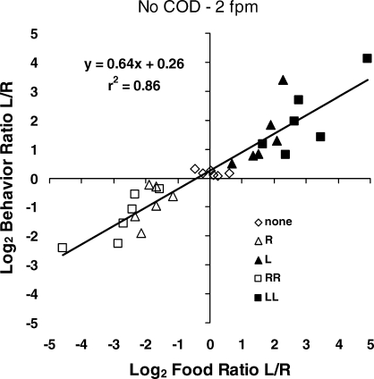
The similarity of the upper and lower graphs in Figure 13 suggests that the shifts in relative likelihood of food might have been discriminable and might have determined the shifts in choice; choice may have tracked food allocation. Figure 14 tests this idea by plotting behavior allocation against food allocation for each pair of points in Figure 13. The fit is good (r²  =  .88), although the slope of the regression line (0.64) indicates considerable undermatching. This result suggests that choice did track food allocation, but that the shifts in choice underestimated the shifts in relative likelihood of food. Comparing Figure 14 with the lower graph in Figure 12, we see similar relations between choice and food allocation, but at different time scales. Figure 14 shows the relation at a smaller time scale than Figure 12. The slope of the line in Figure 14 is steeper because the dynamics between food deliveries were substantial; choice varied over a wide range within the preference pulse, and measuring choice across an interfood interval, as in Figure 12, averages across the preference pulse. Nevertheless, the two relations resemble one another, and both resemble the highly extended relation shown in Figure 6. Thus, one might consider the three graphs together to represent self-similarity across time scales.

Fig 14.

Choice tracking relative food in the Baum and Davison (2004) experiment. The log behavior ratios from Figure 13 plotted against the log food ratios. The regression line indicates that choice tended to match relative food but with considerable undermatching. This result may be interpreted as an example of self-similarity across time scales.

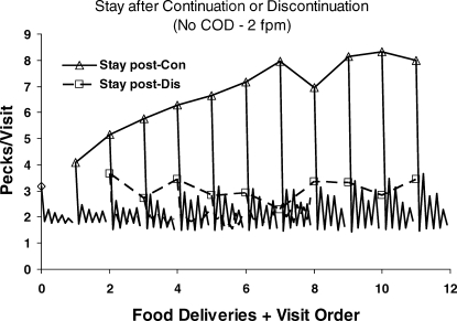
For an example of reduction, we shift to a still smaller time scale: the scale of visits, bouts, or switches, as in Figure 10. As in Figure 13, we look between food deliveries, at bouts following one food delivery and before the next food delivery. Figure 15 shows visits to the just-productive key and switches thereafter; switches immediately following food are omitted, because they were relatively rare (Baum & Davison, 2004). A visit was defined as the series of pecks beginning with food or a switch up to the next switch. Thus, visits were of two types: postfood and postswitch. Visits were averaged in a way similar to the averaging in the preference pulses, across sessions and components according to the sequence of food deliveries (left and right) preceding. Postfood visits were always longer than postswitch visits. Each triangle shows the mean postfood visit following a number of food deliveries in a row from the same key (continuations). The lines without symbols descending from the triangle show the subsequent nine postswitch visits. The first triangle and lines below it show the 10 visits following the first food in any component. The second triangle and lines below it show the 10 visits following two food deliveries in a row from the same key, and so on. A distinct dynamical pattern is evident. The triangle indicates a long postfood visit to the just-productive key, and the line below the triangle shows the first brief postswitch visit to the not-just-productive key, then the following postswitch visit to the just-productive key, which is short but a little longer than the visit to the not-just-productive key, and so on. The saw-tooth pattern shows that, as responding switched back and forth between keys, postswitch visits to the just-productive key remained longer than postswitch visits to the not-just-productive key. Indeed, visits to the not-just-productive key were always about the same—between 1.5 and 1.8 pecks—indicating that many of these consisted of a single peck, consistent with the fix-and-sample pattern (Figure 9). As more food continued to be delivered from the same key, the dynamical pattern expanded, becoming roughly stable after eight deliveries in a row. The line beginning with a diamond at zero on the x-axis shows that this dynamical pattern was visible to some extent even before any food delivery, when analysis begins with whichever key was pecked first at the beginning of the component.

Fig 15.

Visits or bouts within components in the Baum and Davison (2004) experiment. Triangles show the first visit at a key following a series of 1 to 11 food deliveries from that same key (continuations). The lines extending down from the triangles show visits following that visit, alternating between the not-just-productive key and the just-productive key. A dynamic pattern of long visit followed by shorter alternating visits appears following the first food delivery and becomes more pronounced with further continuations. The line beginning with a diamond at zero on the x-axis shows the pattern in visits before any food when visits are calculated from the first key pecked. The squares show the first visit following a food delivery from the other key—a discontinuation. The dynamic pattern is apparent only at first, when only one food delivery preceded the switch of key; when preceded by more than one continuation, the postfood visit is relatively short, and the postchangeover visits at both keys are shorter still, indicating rapid alternation. These dynamics present an example of reduction at a small time scale.

The squares in Figure 15 show the postfood visit following a discontinuation—one or more food deliveries from one key followed by a delivery from the other key. They are much shorter than the postfood visits after continuations (triangles). The same dynamical pattern appears in much attenuated form except for the first square, the discontinuation following one prior delivery on the other key (left–right or right–left; 2 on the x-axis). Beyond that, the saw-tooth pattern disappears, although the postswitch visits following the postfood visit are shorter and close to the minimal visits (about two pecks per visit). The more prior continuations, the less patterning appears in the visits following the discontinuation.

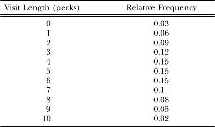
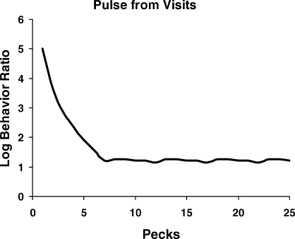
Figure 15 is an example of reduction because the dynamics evident in the switching, even though they reflect preference between the keys, bear no resemblance to the matching law that appears in Figure 14. We cannot derive the switching patterns in Figure 15 from the preference pulses in Figure 13, but we can derive the preference pulses from the switching patterns. To illustrate, we can create a simple model of visits as follows. Assume that postfood visits are relatively long on average—0 to 10 pecks, with a frequency distribution as shown in Table 1. Such a distribution roughly approximates ones that actually occur, except that the real ones have a tail beyond 10-peck visits (Aparicio & Baum, 2006; Baum & Davison, 2004). Assume that postswitch visits are shorter—just 1 or 2 (equally often) at the not-just-productive key and 3 or 4 pecks (equally often) at the just-productive key. We construct visit sequences as follows. Each of the 11 postfood visits is followed by two postswitch sequences, 1–4 and 2–3. These 22 visit sequences specify 22 peck sequences. These are taken out to 25 pecks, assigning frequencies to the sequences according to the frequency distribution. For each ordinal peck following food, we sum the frequencies of pecks on the left key and pecks on the right key across the 22 sequences following a left food delivery and calculate the left–right ratio of first pecks, second pecks, and so on, up to 25^th pecks. The result appears in Figure 16. This simple model suffices to produce the shape of the preference pulse. That we can derive the preference pulse from the visits, but not the other way around, shows that we can reduce choice to switching patterns.

Table 1.

The frequency distribution of postfood visit length used in the model generating Figure 16, a preference pulse, from visits or switches.

Fig 16.

An approximation to a preference pulse derived from a simple model of the switching dynamics shown in Figure 15. The preference pulse, and hence matching, can be derived from the switching dynamics, but not the other way around.

Figure 16 implies that bouts or switches represent a smaller time scale than preference pulses. This ordering might seem counterintuitive because the pulses are calculated peck by peck. The pecks, however, stand in for time—each one represents a unit of time, and the pulse can be calculated using instead a small time unit such as a second or two. Calculation of the pulse ignores switches, blurring the different visits and averaging across them, whereas the switches ending the visits are brief events associated with just one key. The length of visits to a key depends on the probability of a switch to the other key, and that switch is an event on a smaller time scale than the time units of the pulse.

Conclusion

Self-similarity, or scale invariance, may occur across all time scales or across all but the smallest. Reduction occurs as one examines the dynamics of choice at the smallest time scales. One might be tempted to consider the relations at the smallest time scale to be somehow “fundamental,” and the traditional molecular view of behavior would privilege a small scale that seemed to coincide with its assumptions of discrete momentary events and contiguity (Baum, 2002; 2004). The molar view, however, considers the regularities at all time scales to be relevant and valid. None is “fundamental,” because any may be interesting or useful. Practical considerations or apparatus limitations might favor research or application at any time scale. In applied behavior analysis, in particular, regularities on the smallest time scale may be of little use or interest (Baum, 2003). When one is dealing with problem behavior in a classroom, for example, delivering a teacher's attention or praise at precise moments may be impractical and, in any case, a relation at a longer time scale may suffice. Thus, applied problems may require intervention on a relatively long time scale as a practical matter, and interventions on a small time scale might actually prove less effective. In sum, for the study of behavior at various time scales, adopting the molar view is most helpful (Baum, 2002; 2004).

REFERENCES

- Aparicio C.F, Baum W.M. Fix and sample with rats in the dynamics of choice. Journal of the Experimental Analysis of Behavior. 2006;86:43–63. doi: 10.1901/jeab.2006.57-05. [DOI] [PMC free article] [PubMed] [Google Scholar]
- Aparicio C.F, Baum W.M. Dynamics of choice: Relative rate and amount affect local preference at three different time scales. Journal of the Experimental Analysis of Behavior. 2009;91:293–317. doi: 10.1901/jeab.2009.91-293. [DOI] [PMC free article] [PubMed] [Google Scholar]
- Banna K.M, Newland M.C. Within-session transitions in choice: A structural and quantitative analysis. Journal of the Experimental Analysis of Behavior. 2009;91:319–335. doi: 10.1901/jeab.2009.91-319. [DOI] [PMC free article] [PubMed] [Google Scholar]
- Baum W.M. The correlation-based law of effect. Journal of the Experimental Analysis of Behavior. 1973;20:137–153. doi: 10.1901/jeab.1973.20-137. [DOI] [PMC free article] [PubMed] [Google Scholar]
- Baum W.M. On two types of deviation from the matching law: Bias and undermatching. Journal of the Experimental Analysis of Behavior. 1974;22:231–242. doi: 10.1901/jeab.1974.22-231. [DOI] [PMC free article] [PubMed] [Google Scholar]
- Baum W.M. Time-based and count-based measurement of preference. Journal of the Experimental Analysis of Behavior. 1976;26:27–35. doi: 10.1901/jeab.1976.26-27. [DOI] [PMC free article] [PubMed] [Google Scholar]
- Baum W.M. Matching, undermatching, and overmatching in studies of choice. Journal of the Experimental Analysis of Behavior. 1979;32:269–281. doi: 10.1901/jeab.1979.32-269. [DOI] [PMC free article] [PubMed] [Google Scholar]
- Baum W.M. Optimization and the matching law as accounts of instrumental behavior. Journal of the Experimental Analysis of Behavior. 1981;36:387–403. doi: 10.1901/jeab.1981.36-387. [DOI] [PMC free article] [PubMed] [Google Scholar]
- Baum W.M. Quantitative prediction and molar description of the environment. The Behavior Analyst. 1989;12:167–176. doi: 10.1007/BF03392493. [DOI] [PMC free article] [PubMed] [Google Scholar]
- Baum W.M. From molecular to molar: A paradigm shift in behavior analysis. Journal of the Experimental Analysis of Behavior. 2002;78:95–116. doi: 10.1901/jeab.2002.78-95. [DOI] [PMC free article] [PubMed] [Google Scholar]
- Baum W.M. The molar view of behavior and its usefulness in behavior analysis. The Behavior Analyst Today. 2003;4:78–81. [Google Scholar]
- Baum W.M. Molar and molecular views of choice. Behavioural Processes. 2004;66:349–359. doi: 10.1016/j.beproc.2004.03.013. [DOI] [PubMed] [Google Scholar]
- Baum W.M, Davison M. Choice in a variable environment: Visit patterns in the dynamics of choice. Journal of the Experimental Analysis of Behavior. 2004;81:85–127. doi: 10.1901/jeab.2004.81-85. [DOI] [PMC free article] [PubMed] [Google Scholar]
- Baum W.M, Davison M. Modeling the dynamics of choice. Behavioural Processes. 2009;81:189–194. doi: 10.1016/j.beproc.2009.01.005. [DOI] [PubMed] [Google Scholar]
- Baum W.M, Schwendiman J, Bell K.E. Choice, contingency discrimination, and foraging theory. Journal of the Experimental Analysis of Behavior. 1999;71:355–373. doi: 10.1901/jeab.1999.71-355. [DOI] [PMC free article] [PubMed] [Google Scholar]
- Belke T.W, Heyman G.M. Increasing and signaling background reinforcement: Effect on the foreground response–reinforcer relation. Journal of the Experimental Analysis of Behavior. 1994;61:65–81. doi: 10.1901/jeab.1994.61-65. [DOI] [PMC free article] [PubMed] [Google Scholar]
- Davison M, Baum W.M. Choice in a variable environment: Every reinforcer counts. Journal of the Experimental Analysis of Behavior. 2000;74:1–24. doi: 10.1901/jeab.2000.74-1. [DOI] [PMC free article] [PubMed] [Google Scholar]
- Davison M, Baum W.M. Choice in a variable environment: Effects of blackout duration and extinction between components. Journal of the Experimental Analysis of Behavior. 2002;77:65–89. doi: 10.1901/jeab.2002.77-65. [DOI] [PMC free article] [PubMed] [Google Scholar]
- Davison M, Baum W.M. Every reinforcer counts: Reinforcer magnitude and local preference. Journal of the Experimental Analysis of Behavior. 2003;80:95–129. doi: 10.1901/jeab.2003.80-95. [DOI] [PMC free article] [PubMed] [Google Scholar]
- Davison M, Baum W.M. Do conditional reinforcers count. Journal of the Experimental Analysis of Behavior. 2006;86:269–283. doi: 10.1901/jeab.2006.56-05. [DOI] [PMC free article] [PubMed] [Google Scholar]
- Davison M, Baum W.M. Local effects of delayed food. Journal of the Experimental Analysis of Behavior. 2007;87:241–260. doi: 10.1901/jeab.2007.13-06. [DOI] [PMC free article] [PubMed] [Google Scholar]
- Davison M.C, Hunter I.W. Concurrent schedules: Undermatching and control by previous experimental conditions. Journal of the Experimental Analysis of Behavior. 1979;32:233–244. doi: 10.1901/jeab.1979.32-233. [DOI] [PMC free article] [PubMed] [Google Scholar]
- Gallistel C.R, Mark T.A, King A.P, Latham P. The rat approximates an ideal detector of changes in rates of reward: Implications for the law of effect. Journal of Experimental Psychology: Animal Behavior Processes. 2001;27:354–372. doi: 10.1037//0097-7403.27.4.354. [DOI] [PubMed] [Google Scholar]
- Gallistel C.R, King A.P, Gottlieb D, Balci F, Papachristos E.B, Szalecki M, et al. Is matching innate. Journal of the Experimental Analysis of Behavior. 2007;87:161–199. doi: 10.1901/jeab.2007.92-05. [DOI] [PMC free article] [PubMed] [Google Scholar]
- Hall G. Behaviour: An introduction to psychology as a biological science. London: Academic Press; 1983. [Google Scholar]
- Hunter I, Davison M. Determination of a behavioral transfer function: White-noise analysis of session-to-session response-ratio dynamics on concurrent VI VI schedules. Journal of the Experimental Analysis of Behavior. 1985;43:43–59. doi: 10.1901/jeab.1985.43-43. [DOI] [PMC free article] [PubMed] [Google Scholar]
- Kyonka E.G.E, Grace R.C. Rapid acquisition of preference in concurrent chains when alternatives differ on multiple dimensions of reinforcement. Journal of the Experimental Analysis of Behavior. 2008;89:49–69. doi: 10.1901/jeab.2008.89-49. [DOI] [PMC free article] [PubMed] [Google Scholar]
- Mark T.A, Gallistel C.R. Kinetics of matching. Journal of Experimental Psychology: Animal Behavior Processes. 1994;20:79–95. [PubMed] [Google Scholar]
- Mazur J.E. Choice behavior in transition: Development of preference with ratio and interval schedules. Journal of Experimental Psychology: Animal Behavior Processes. 1992;18:364–378. doi: 10.1037//0097-7403.18.4.364. [DOI] [PubMed] [Google Scholar]
- Rachlin H. Behavior and mind: The roots of modern psychology. New York: Oxford University Press; 1994. [Google Scholar]
- Schofield G, Davison M. Nonstable concurrent choice in pigeons. Journal of the Experimental Analysis of Behavior. 1997;68:219–232. doi: 10.1901/jeab.1997.68-219. [DOI] [PMC free article] [PubMed] [Google Scholar]