Modelling temporal evolution of cardiac electrophysiological features using Hidden Semi-Markov Models

Abstract

This paper presents a new method to analyse cardiac electrophysiological dynamics. It aims to classify or to cluster (i.e. to find natural groups) patients according to the dynamics of features extracted from their ECG. In this work, the dynamics of the features are modelled with Continuous Density Hidden Semi-Markovian Models (CDHSMM) which are interesting for the characterization of continuous multivariate time series without a priori information. These models can be easily used for classification and clustering. In this last case, a specific method, based on a fuzzy Expectation Maximisation (EM) algorithm, is proposed. Both tasks are applied to the analysis of ischemic episodes with encouraging results and a classification accuracy of 71%.

I. INTRODUCTION

The analysis of ECG signals for the caracterization of various cardiovascular pathologies is usually based on the extraction of several features such as magnitude of the ECG waves, duration of the QRS complex, QT interval or cardiac rhythm.

The diagnosis is generally based on these features, but without taking into account their temporal evolution. In this work, we propose to model the dynamics of the features with Continuous Density Hidden Semi-Markovian Models (CDHSMM). HMM, which have been extensively used in speech processing, present many interesting particularities: they are able to represent the dynamics in a compact model, very few hyper-parameters have to be tuned and reliable methods are available to learn the model parameters. Thanks to the probabilistic approach, HMM are here used for classification purposes, according to the maximum likelihood.

The clustering problem is also adressed. Clustering time series with HMM is not new. Three different techniques exist: (1) hierarchical clustering and down-top approach, it begins with one HMM per time series and successively merges series according to a distance measure between HMM; (2) top-down approach, it begins with one or two HMM and creates new models from the time series which have low likelihood to be generated by the current models; (3) hybrid approach, it begins with a hierarchical clustering (for example with a distance based on Dynamic Time Warping) and then uses a classical top-down approach with the HMM. The proposed contribution can be viewed as an extension of the top-down approach where CDHSMM and fuzzy membership are introduced.

The first section presents the different methodology steps, starting from the ECG and arriving to the patients classification and/or clustering according to the observed dynamics. The way in which these dynamics are modelled is detailed section 2, where a description of the model structure, the learning method and the estimation of the hyper-parameters are presented. In section 3, the clustering approach is described step by step. Finally, the last section is dedicated to classification and clustering of ischemic episodes.

II. General Procedure

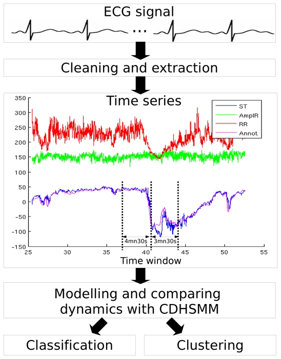
Figure 1 summarizes the general procedure used to analyse the cardiac electrophysiological dynamics. The ECG acquired during various tests (effort and tilt tests, Holter recordings…) are cleaned and relevant features are extracted [1], thus creating multivariate time series.

Fig. 1.

General process of the proposed methodology based on CDHSMM.

In a learning phase, the CDHSMM models are adjusted on a subset of these time series X = {O₁, O₂, …, O_N} (O_i is one time series and N is the number of time series). This step aims to maximise the probability P(X|θ) where θ defines the model parameters:

$${\theta }_{\mathit{opt}}=\underset{\theta }{\text{argmax}}\{P(X\mid \theta )\}$$

In a test phase, the likelihood that a time series has been generated by an existing model with parameters θ, P(O_i|θ), is computed.

Based on the learning and test phases, the classification assigns a time series to the model index k_win which gives the highest likelihood:

$$k_{\mathit{win}}=\underset{\text{1}\le k\le K}{\text{argmax}}\{P(O_i,{\theta }_k)\}$$

where K is the number of competitive models.

On the other side, the clustering carries out several iterations of the learning and test phases, in order to retrieve the natural time series classes.

III. CDHSMM modelling

CDHSMM [2] is the most common specialisation of HMM for modelling continuous time series. For a good understanding, this section details the structure of the model, the initialisation step, the learning phase and the definition of the hyper-parameters.

A. structure of the model

CDHSMM’s states differ from standard HMM’s states by two points. Indeed, each state:

• represents a subspace of the observation distributions. To reduce computation time, these distributions (multi-dimensional in our case) are formulated as a multivariate Gaussian probability density function [3].

• models its duration probability with a Gaussian probability function. In this case, duration densities do not decrease exponentially with time as in standard HMM. It is thus suited to continuous signals, where the state durations can be quite long.

According to [4], using only one Gaussian is equivalent of using a mixture of Gaussian but with less states. Thus, for simplicity, only one Gaussian is considered. Finally, the model is defined by one hyper-parameter S (the number of states of the model) and the set of parameters θ, θ = {π_i, a_{i j}, b_i(μ⃗, σ), pd_i(μ_d, σ_d)} where π_i are the initial probabilities, a_{i j} are the transition matrix coefficients, b_i(μ⃗, σ) are the multivariate gaussian probability density functions of each state (μ⃗ is the mean vector and Σ is the covariance matrix), pd_i(μ_d, σ_d) are the parametric gaussian distributions of the time duration in each state (μ_d, σ_d are respectively the mean and the standard deviation).

B. Initialisation and learning the parameters of the model

The initialisation of the state’s emission probability, b_i(μ⃗, σ) is done with a spatial clustering based on Gaussian Mixtures Models (GMM). Each component of the GMM will correspond to one state. Uniform probabilities are set to a_{i j} and π_i. The estimation of the pd_i(μ_d, σ_d) distributions starts with the training of a CDHMM, then the most plausible paths are determined on the time series and an estimation of the time spent in each state can be computed.

In the clustering process, models have to be iteratively trained and a fast procedure for learning θ is required. In consequence, the Viterbi algorithm [5] has been chosen instead of the standard Baum-Welch algorithm [6] which is recognized to be time consuming.

C. Definition of the hyper-parameters

The number of states S is the only hyper-parameter to adjust. Creating models with the appropriate number of states is not a trivial problem: a model with too much states will over-fit the observations, while a model with too few states will wrongly describe the time series that should belong to this model. Many methods have been proposed to estimate S. They consist in approximating the marginal likelihood of the observations P(X|S) defined as:

$$P(X\mid S)={\int }_{\theta }P(X\mid \theta ,S)P(\theta \mid S)d\theta$$ (1)

by some popular approaches such as the Laplace approximation [7], the Bayesian Information Criterion [8] or the Cheeseman-Stutz approximation [9]. Due to the iterative scheme of the clustering algorithm, the BIC approximation, which is less time consuming, has been retained:

$$S_{\mathit{opt}}=\underset{S}{\text{argmax}}(\mathit{logP}(X\mid S,\widehat{\theta }(S))-f(S)/2\ast \mathit{logN})$$ (2)

where f(S) returns the number of parameters according to the number of states. Finally, to avoid the problem due to initialisation, the probability P(X|S,θ̂(S)) is computed 20 times and the average value is considered.

IV. Clustering process

Clustering aims to retrieve the different natural groups of the observed time series. As mentioned previously, the top-down approach has been retained. Justifications and details about this approach are presented in the next subsections.

A. Top-Down approach

A top-down approach has been chosen for two main reasons:

1. In clustering tasks, the number K of clusters is usually small compared to the number of individuals (in our case an individual is a multivariate continuous time series). Thus, it seems natural to initialise the process with a small number of clusters. A small number of clusters will also ensure to group together individuals with respect to the main global dynamics.

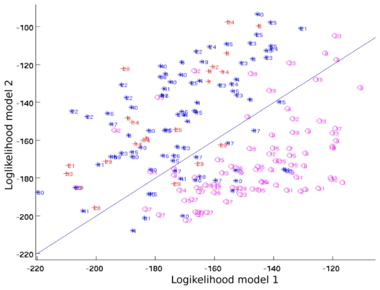
2. The loglikelihood of all the models can be used to define a featuring space (see figure 4 for example) of small dimension based on the dynamics and where all the time series can be easily embedded and compared. This can be opposed to hierarchical clustering where a distance between all pairs of models is computed, which is time consuming.

Fig. 4.

Clustering result with two models. o points are the ST-AS episodes, * are the ST-IS episodes and + are the ST-RC episodes.

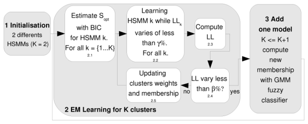
Our clustering process is organised, as depicted figure 2, in several steps.

Fig. 2.

Top-down clustering with fuzzy Expectation Maximization.

• Step 1: Initialisation: random assignment of all the time series to two different CDHSMMs.

• Step 2.1: Learning the number of states S_opt for each CDHSMM with the BIC criteria: for simplicity the BIC is computed only at the first iteration of the EM loop.

• Step 2.2: Learning each model with the Viterbi Algorithm (VA): the VA takes into account the membership of each individuals (equation 6). The computation of the cluster k likelihood integrates also this membership:

  $${LL}_k=P(\sum _{i}P(k\mid O_i,\mathrm{\Lambda })\mathit{logP}(O_i\mid {\widehat{\theta }}_k))$$ (3)

  Λ denotes the mixture of the K CDHSMM. The convergence is assumed when LL_k varies less than α = 0.01% from one iteration to the next.

• Step 2.3: Computing the full partition likelihood (LL) by integrating the likelihood on all the clusters and all the time series, let:

  $$LL=\mathit{logP}(X\mid \mathrm{\Lambda })=\sum _i\mathit{log}(\sum _k{\alpha }_{k}P(O_i\mid {\theta }_k))$$ (4)

• Step 2.4: Testing the convergence of the EM process: if LL does not vary from one iteration to the next, of more than β = 0.1%, it is assumed that the mixture of a CDHSMMs has been sufficiently fitted and a new cluster is added. Otherwise, another iteration of the EM is performed.

• Step 2.5: Updating the weights of each clusters (α_k) and the membership of each individual by applying equations 5 and 7.

• Step 3: Inserting a new cluster: the likelihood space proposes a good featuring space for representing the time series. With a K+1 gaussian mixtures model, it is easy to cluster this featuring space with an additional model, while keeping a fuzzy membership.

B. EM partitioning with fuzzy membership

The membership of a time series to a cluster (i.e. to a CDHSMM) is given by its prior probability to belong to this cluster and taking into account the current partitioning, let:

$$P(k\mid O_i,\mathrm{\Lambda })=\frac{{\alpha }_{k}P(O_i\mid {\theta }_k)}{{\mathrm{\sum }}_j{\alpha }_{j}P(O_i\mid {\theta }_j)}$$ (5)

this probability is integrated in the maximisation step when updating parameters of each HSMM:

$${\widehat{\theta }}_k=\underset{{\theta }_k}{\text{argmax}}\sum _{i}P(k\mid O_i,\mathrm{\Lambda })\mathit{logP}(O_i\mid {\theta }_k)$$ (6)

whereas α_k, the weight of each cluster, is updated with:

$${\alpha }_k^{\mathit{new}}=\frac{1}{N}\sum _{n}P(k\mid O_i,\mathrm{\Lambda })$$ (7)

This procedure avoids hard assignation of one particular time series, with probability equal to 1 to a given cluster and 0 to the others, which can lead to a biased convergence.

V. Results

The ECG records come from the LTST database [10], which is dedicated to the assessment of ischemic episodes classification algorithms. The detection of ischemia is traditionally based on ST-segment deviations. This feature presents a low specificity because other causes, such as heart rate increasing or position changes, can induce the same kind of deviations. In this database, experts annotated several ST-segment deviations into three classes:

• Transitory ST episodes compatible with ischemia, ST-Ischemia (ST-IS). They are distinguished by changes in the ST-segment morphologies, potentially accompanied with changes in the heart rate. Clinical information suggesting ischemia are taken into account.

• Non-ischemic ST episodes due to cardiac rhythm changes, ST-Rhythm Change (ST-RC). They are distinguished by changes in the ST-segment morphologies, potentially accompanied with changes in heart rate and when clinical informations do not suggest ischemia.

• ST episodes due to position changes of the patient, ST-Axis shift (ST-AS). They are characterized by abrupt or progressive changes of morphologies of the ST segment, accompanied with amplitude changes of the QRS waves.

A. Modelling

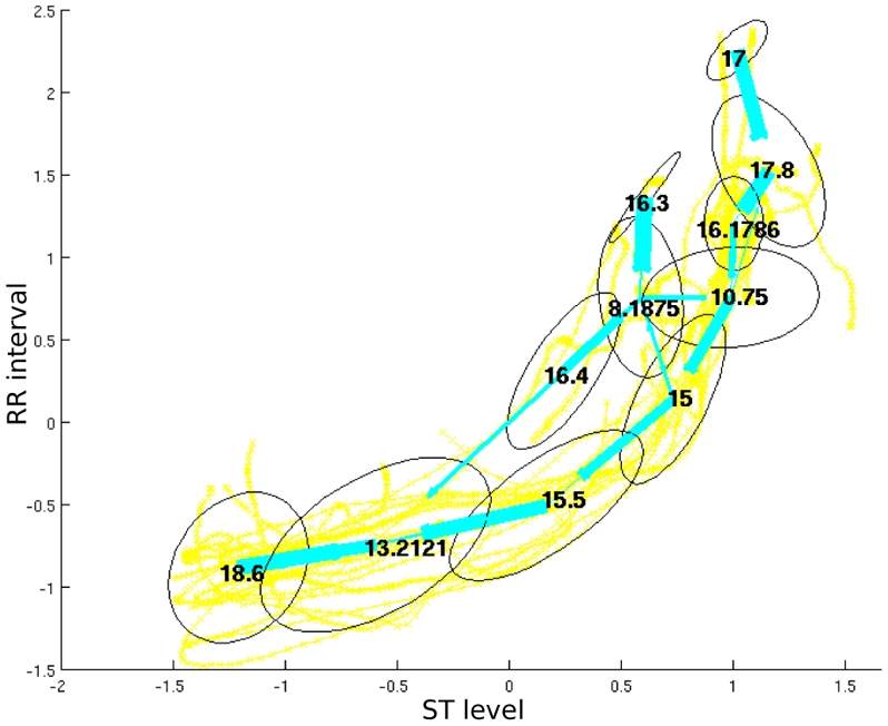
An exemple of the modelling achieved with the CDHSMM on 15 bivariate (ST level and RR interval) time series extracted from LTST database is presented on figure 3.

Fig. 3.

ST levels/RR-intervals normalized trajectories of 15 ST-IS episodes modelled with a CDHSMM: the ellipses represent the bivariate gaussians assigned to each state, the straight lines represent the transitions between the states, the numbers into the ellipses are the state time duration means.

B. Classification

We aim to classify the ST change episodes. The beginning of each episode, which is identified when the ST deviation exceeds a threshold V_min and during a minimum time T_min, is annotated in the database and used as a reference to model the time series. For the classification step, it has been empirically observed that:

1. the following variables V = {ST deviations, RR intervals, amplitudes of the R and T waves},

2. the modelling time window, starting 4mn 30s before the beginning of the episode and of a total length of 8 minutes (figure 1)

provide the best results. In these conditions, the BIC equation (2) suggests a model with 38 states. With a random training and test sets of respectively 2/3 and 1/3 of the ST episodes, the classification rates obtained on the test set are presented table I. Comparing these rates with those reported in [11], we observed an improvement of 17.7% (53.3% of accuracy in [11], 71% in our case).

TABLE I.

Results of classification on the test episodes, the last column are the sensitivity published in [11]

Classified as
	ST-IS	ST-AS	ST-RC	Sensitivity	Sensitivity (ZI)
ST-IS	852	163	95	76.8%	80.6%
ST-AS	402	1166	82	70.7%	48.6%
ST-RC	150	42	228	54.3%	33.3%

C. Clustering

Figure 4 represents the output of the clustering process with two models. The experimental conditions (variables and time windows) are identical to those used in the classification procedure.

The clustering into two groups is clearly visible: ST-AS episodes in one hand and ST-RC, ST-IS episodes in the other hand. ST-RC events are merged with ST-IS events. This result can be explained by the fact that the ST-RC episodes group is a mixture of patients suffering of various pathologies (mitral stenosis, Wolf-Parkinson-White syndrome, hypertension,…).

VI. CONCLUSION

A full methodology for classifying and clustering electrophysiological dynamics observed from the ECG signal has been proposed. The modelling of the temporal evolution of the features is efficiently carried out with CDHSMM models. It has been firstly applied to the classification of ST-episodes observed in Holter recordings. The proposed methodology is able to select the best features and the most adequate analysing window that permit an optimal classification. In these conditions, the classification accuracy has been inscreased of 17.7% compared to [11]. In a second step, clustering has been applied to the ST-episodes to retrieve the natural groups. We bring to light that the ST-AS episodes are clearly separated in the loglikelihood featuring space, compared to the ST-IS and ST-RC episodes. It is worthy to remind that the proposed methodology is generic. It could be applied to other cardiac diseases where temporal evolution must be taken into account. For example, we are currently working on the classification of symptomatic and asymptomatic patients suffering from Brugada’s syndrome.

References

- 1.Dumont J, Hernandez AI, Carrault G. Parameter optimization of a wavelet-based electrocardiogram delineator with an evolutionary algorithm. Computers in Cardiology, 2005. 2005;32:707–710. [Google Scholar]
- 2.Levinson SE. Continuously variable duration hidden markov models for automatic speech recognition. Computer Speech and Language. 1986;1:29–45. [Google Scholar]
- 3.Rabiner L. A tutorial on hidden markov models and selected applications in speeach recognition. Proc of the IEEE. 1989;77(2):257–285. [Google Scholar]
- 4.Bicego M, Murino V, Figueiredo M. A sequential pruning strategy for the selection of the number of states in hidden markov models. Pattern Recognition Letters. 2003;24:1395–1407. [Google Scholar]
- 5.Forney GD. The Viterbi algorithm. Proc IEEE. 1973;61:268–278. [Google Scholar]
- 6.Baum LE, Petrie T, Soles G, Weiss N. A maximisation technique occurring in the statistical analysis of probabilitic functions of Markov chains. Annals Math Stat. 1970;41(1):164–171. [Google Scholar]
- 7.Heckerman D, Geiger D, Chickering DM. A tutorial on learning with bayesian networks. Machine Learning. 1995;20:197–243. [Google Scholar]
- 8.Schwarz G. Estimating the dimension of a model. Annuals of Statistics. 1978;6:461–464. [Google Scholar]
- 9.Cheeseman P, Stutz J. Advances in Knowledge discovbery and data-mining, chapter Bayesian classification (autoclass): Theory and results. Cambridgre, MA: MIT press; 1996. pp. 153–180. [Google Scholar]
- 10.Jager Franc, Taddei Alessandro, Moody George B, Emdin Michele, Antolic Gorazd, Dorn Roman, Smrdel Ales, Marchesi Carlo, Mark Roger G. Long-term ST database: a reference for the development and evaluation of automated ischaemia detectors and for the study of the dynamics of myocardial ischaemia. Medical Biological Engineering Computing. 2003;41(2):172–183. doi: 10.1007/BF02344885. [DOI] [PubMed] [Google Scholar]
- 11.Zimmerman MW, Povinelli RJ, Johnson MT, Ropealla KM. A reconstructed phase space approach for distinguishing ischemic from non-ischemic ST changes using Holter ECG data. Computers in Cardiology, 2003. 2003;30:707–710. [Google Scholar]