Digital Analysis and Sorting of Fluorescence Lifetime by Flow Cytometry

Abstract

Frequency-domain flow cytometry techniques are combined with modifications to the digital signal processing capabilities of the Open Reconfigurable Cytometric Acquisition System (ORCAS) to analyze fluorescence decay lifetimes and control sorting. Real-time fluorescence lifetime analysis is accomplished by rapidly digitizing correlated, radiofrequency modulated detector signals, implementing Fourier analysis programming with ORCAS’ digital signal processor (DSP) and converting the processed data into standard cytometric list mode data. To systematically test the capabilities of the ORCAS 50 MS/sec analog-to-digital converter (ADC) and our DSP programming, an error analysis was performed using simulated light scatter and fluorescence waveforms (0.5–25 ns simulated lifetime), pulse widths ranging from 2 to 15 µs, and modulation frequencies from 2.5 to 16.667 MHz. The standard deviations of digitally acquired lifetime values ranged from 0.112 to >2 ns, corresponding to errors in actual phase shifts from 0.0142° to 1.6°. The lowest coefficients of variation (<1%) were found for 10-MHz modulated waveforms having pulse widths of 6 µs and simulated lifetimes of 4 ns. Direct comparison of the digital analysis system to a previous analog phase-sensitive flow cytometer demonstrated similar precision and accuracy on measurements of a range of fluorescent microspheres, unstained cells and cells stained with three common fluorophores. Sorting based on fluorescence lifetime was accomplished by adding analog outputs to ORCAS and interfacing with a commercial cell sorter with a radiofrequency modulated solid-state laser. Two populations of fluorescent microspheres with overlapping fluorescence intensities but different lifetimes (2 and 7 ns) were separated to ~98% purity. Overall, the digital signal acquisition and processing methods we introduce present a simple yet robust approach to phase-sensitive measurements in flow cytometry. The ability to simply and inexpensively implement this system on a commercial flow sorter will both allow better dissemination of this technology and better exploit the traditionally underutilized parameter of fluorescence lifetime.

1. Introduction

Time-resolved methods in flow cytometry were introduced almost two decades ago, and upon their inception high-throughput measurements of fluorescence decay kinetic parameters were established (1–3). In particular, the average fluorescence lifetime, measured on an event-by-event basis, was used as an independent parameter in cell cycle analysis, quenching studies, free-dye experiments, and other assays to discriminate between fluorophores with closely overlapping emission spectra (3–6). Although a powerful indicator of details affecting fluorescence, the excited state lifetime is largely underutilized by cytometrists. The average fluorescence lifetime can provide a quantitative measure of fluorophore environment yet is not measurable by commercial cytometry instruments, primarily due to the expense and complexity of previous implementations. The height, area, and width of fluorescence intensity pulses have prevailed as parameters for high-throughput cell cycle analysis, immunophenotyping, fluorescent protein analyses, cell sorting, bead-based assays and many other cytometry applications.

Despite improvements in the ability to separate populations based on intensity alone, the average fluorescence decay time remains a strategic element for flow cytometry applications. For example, lifetime measurements are unique and independent indicators of fluorescence quenching and enhancement; early studies demonstrated the ability of lifetime to evaluate fluorophore-antibody ratios and the total number of receptor sites on the cell surface (4). Lifetime was necessary for quantitative measurements of such ratios because of non-linear intensity measurements due to self-quenching at high fluorophore concentrations. In cell cycle studies, lifetime measurements have proven essential in discriminating DNA and/or RNA content because single exponential decay is a parameter independent of background dye, unbound drug, and differences in spectrally overlapping DNA or RNA binding dyes (5–9). Lifetime measurements are also very relevant in current flow cytometry applications that utilize autofluorescence as a negative control. The lifetime parameter can clearly distinguish between exogenous and endogenous fluorescence, even when they are similar in both intensity and emission wavelength. The use of phase-filtering methods (11) can markedly reduce the cellular autofluorescence signal that is a background for exogenous fluorophores. Overall, new opportunities for fluorescence lifetime as an independent parameter continue to emerge as cytometry assays become increasingly complex; nowhere was this better foreshadowed than by Keij et al. who resolved a set of 20 dual-color fluorescence microspheres using excited singlet state lifetimes over ten years ago (10).

Although fluorescence lifetime is already of great value in image microscopy, the use of fluorescence decay in flow cytometry depends on robust methods to accurately measure time-dependent phenomena in flow. Steinkamp et al. were early pioneers of robust PSFC systems that provided reproducible lifetime measurements with sub-nanosecond resolution (3,11). PSFC uses a frequency-domain method in which the cytometer laser excitation source is intensity-modulated at a single radiofrequency (RF). As a particle passes through the focused, modulated laser beam, fluorescence emission results in a Gaussian-shaped pulse containing an RF modulated intensity component at the same frequency as the modulated excitation source. Owing to the fluorescence decay characteristics of the excited fluorophore, the resulting frequency-modulated component of the fluorescence emission signal is phase-shifted and amplitude-attenuated. Figure 1 depicts the difference between a standard flow cytometry pulse and one that is modulated. The PSFC system accurately quantifies the phase-shift on an event-by-event basis to provide the average fluorescence lifetime of particles in standard FCS file format. In addition to measuring the lifetime of particles, PSFC has also been extensively characterized for free-fluorophore measurements and phase-filtering techniques (2, 11).

Figure 1.

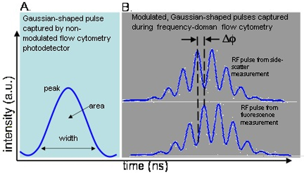
Illustration of A) a normal intensity pulse detected in flow cytometry and B) a modulated pulse detected when acquiring phase-sensitive measurements. The phase shift, ΔΦ, between the modulated fluorescence and side scatter pulse is captured in phase-sensitive flow cytometry to compute the average fluorescence lifetime of the fluorophore or bulk fluorescence species.

PSFC theory, which is described in detail elsewhere (1,3,11), involves homodyne mixing of frequency-modulated emission pulses with reference sinusoids that are phase-shifted. In order to determine in real-time the phase and amplitude of the modulated Gaussian pulses, the signal itself is mixed with both a −90 degree phase-shifted reference quadrature (Q) and a 0 degree in-phase reference signal (I). The Q and I reference signals are sinusoids having the same RF frequency and amplitude as that generated for the excitation source modulation. Subsequent to mixing, the two resultant signals (termed Q_mix and I_mix) are then low-pass frequency filtered and measured. Q_mix and I_mix are proportional to the sine and cosine of the phase-shift (φ), respectively (3). The lifetime (τ) is proportional to tanφ as shown in Equation 1, where ω is the angular modulation frequency.

$$\tau =\frac{\text{tan}\phi }{\omega }$$ (1)

Since the ratio of sinφ over cosφ is equivalent to tanφ, the ratio of the Q_mix and I_mix signals is calculated in analog space, resulting in a signal proportional to the average fluorescence lifetime when assuming single exponential decay kinetics.

The PSFC system, which is depicted in Figure 2, is extremely reliable for determining the average lifetime of an event, yet the complex phase-sensitive electronic, optical, and analog instrumentation control described above have limited the implementation of fluorescence lifetime quantification in modern flow cytometers. Although other novel ideas evolved from the PSFC system, including time-domain techniques (12), frequency-domain heterodyning (13), multi-frequency measurements (14) and digital data acquisition (15,16), most lifetime techniques required either complex data processing, slow data acquisition, or complicated phase mixing. For example, Beisker and Klocke revealed the simplified concept of digital lifetime acquisition based on phase-shift measurements of DNA-intercalated ethidium bromide at different concentrations (16). Yet this method of collecting modulated waveforms with a digital oscilloscope and performing off-line Fourier analysis was not developed in combination with cytometric data acquisition systems, was not capable of phase-sensitive measurements for phase filtering, did not incorporate a rapid fitting routine, and was not high-throughput for reliable lifetime precision.

Figure 2.

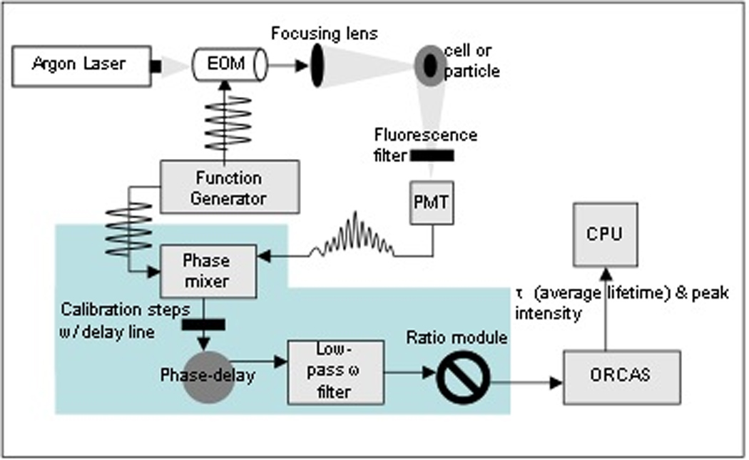
Illustration of the phase-sensitive flow cytometry system constructed by Steinkamp et al. at the NFCR. This depiction assumes the particles are flowing into the page; the analog homodyning hardware (blue) are depicted for only one detector. By adding detectors and performing calibration steps, the analog components comprise a system that is not only complex but also outmoded and expensive.

In this work, we combine early concepts of lifetime cytometry with modern frequency modulation techniques and characterize a system that: (1) digitally captures fluorescence lifetime in real-time with a modified ORCAS (17); (2) matches the accuracy and precision of analog PSFC; and (3) is capable of sorting when retrofitted on a commercial flow sorter. Our characterization of single exponential fluorescence decay-dependent analysis and sorting is described herein with emphasis on the simplicity of translating lifetime measurements to existing commercial flow cytometry instruments.

2. Materials and Methods

2.1 Digital analysis hardware

We have demonstrated digital fluorescence lifetime cytometry with a commercial flow cytometer as well as on the analog PSFC system, originally described and characterized by Steinkamp et al. (11). The PSFC, illustrated in Figure 2, was retrofitted with the digital hardware for direct comparisons between digital and analog lifetime acquisition using the same excitation source, fluidics and detectors. As an analog instrument, the PSFC has an argon-ion laser source (Spectra-Physics Lasers Inc., model 171–19, beam diameter ~5 mm) that is externally intensity modulated with an electro-optic modulator (EOM) (Conoptics Inc., model 355-2P and driver-amplifier model 50). Alternatively, we use a thermoelectrically cooled laser diode that is directly modulated by supplying an RF signal to an internal laser mount bias-T network (Thorlabs Inc., mount model TCLDM9, temperature controller model TED 200, driver model LDC220). The laser intensities range from 100 mW to approximately 400 mW. A digital dual-channel function generator (Tektronix Inc., model AFG 3102) generates a radio-frequency signal (typically 10MHz) that is sent either to the EOM driver-amplifier or the diode mount. A second RF output is digitally generated and sent to a quadrature phase hybrid module for analog phase shifting. Subsequent to modulation, the excitation beam is elliptically shaped by two crossed cylindrical lenses (focal lengths: 30 and 5.4 cm) and then focused onto an inverted flow chamber (cross section 200 µm²: Beckman-Coulter, Inc., Biosense model). Cells or particles are syringe pumped (Chemyx Incorporation Houston, TX, model N3000) into the flow chamber, hydrodynamically focused, and passed through the laser beam at typical flow rate of 10 µL/min. The particle transit time through the Gaussian-shaped laser beam is approximately 15 µs. Fluorescence emission and side scatter are collected at 90° to the excitation direction and focused onto the windows of appropriately filtered photomultiplier tubes (PMT; Hamamatsu, Inc., model R636-10). The signals from the PMTs are amplified using specially designed high-speed, trans-impedance preamplifiers to preserve the high frequency RF component of the signals. Using the analog approach four parameters are measured: (1) the low-pass frequency filtered fluorescence emission pulse height; (2) I_mix; (3) the ratio of parameters Q_mix and I_mix; and (4) the low-pass frequency filtered side scatter pulse height.

When our digital schema is implemented on the traditional PSFC system, the amplified PMT fluorescence and side scatter signals are directly connected to ORCAS (17) so that both modulated-Gaussian pulses are digitized directly; Figure 3 demonstrates this simplicity. The 50 MS/sec sample rate of the ORCAS ADC board is required to accurately capture the high frequency information contained in these signals. Due to the fluorescence decay kinetics of the sample, the modulated-Gaussian fluorescence and side scatter pulses have different phase values, which contain the delay information needed to interpret lifetime on an event-by-event basis. Additionally, the RF signal from the function generator, which is used to modulate the laser, is phase-locked to the ORCAS ADC sample clock; this improves the accuracy of the phase measurement and is used to simplify the phase calculations.

Figure 3.

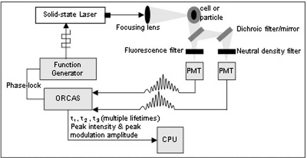
Depiction of the digital lifetime cytometry system illustrated in a geometry, which assumes the particles are flowing into the page. The PMT outputs go directly to the data system for DFT calculations and on-line lifetime acquisition.

2.2 Data processing

The DSP calculates the phase shift between the fluorescence and scatter signals to determine the lifetime. A Discrete Fourier Transform (DFT) is applied to the waveform in order to calculate the phase of the modulation signal, as shown in Equation 2, where I represents the input signal, ω represents the modulation frequency, t represents time, and i is the imaginary unit number.

$$I({\omega }_k)={\displaystyle \sum _{n=0}^{N}I(t_n)\text{exp}(-i{\omega }_k{t}_n)}$$ (2)

We enforce two requirements to simplify the processing of the DFT. The first requirement restricts the frequency of the modulation signal to be the ADC sample rate divided by an integer. This guarantees that one cycle of the modulation frequency is always exactly an integral number of samples from the ADC. The second requirement restricts the length of the captured waveform to be an integer multiple of single cycles of the modulation signal. Combined with the first requirement, this guarantees that the modulation frequency is always located precisely inside one specific frequency “bin” of the DFT, and eliminates any spectral leakage from the modulation signal without the use of a window function. Since one frequency bin is sufficient, the Fourier transform derivation is most efficient; algorithms like the Fast Fourier Transform (FFT) are not necessary. Part of the Fourier transform calculation involves integer math, but eventually multiplication by sine and cosine terms is required which necessitates floating point math. The sine and cosine terms are thus pre-computed for the specific modulation frequency so as to speed the phase calculations significantly. The result of the Fourier transform algorithm is a real part and an imaginary part for the modulation frequency. Therefore after the complex DFT output of each individual waveform is processed by the DSP, the phase, φ, and magnitude, A, can be calculated by Equations 3 and 4, respectively.

$$[{\phi }_F,{\phi }_S]=\text{arctan}\frac{IMAG\left[I{(f_{\text{mod}})}_{F,S}\right]}{REAL\left[I{(f_{\text{mod}})}_{F,S}\right]}$$ (3)

$$[A_F,A_S]=\sqrt{\mathit{\text{IMAG}}{\left[I{(f_{\mathrm{mod}})}_{F,S}\right]}^2+\mathit{\text{REAL}}{\left[I{(f_{\mathrm{mod}})}_{F,S}\right]}^2}$$ (4)

In Equation 3 and Equation 4, I(f_mod) is the maximum output of the frequency spectrum (or single frequency bin), while the subscripts F and S refer to the fluorescence and side scatter signals, respectively. The phase of the fluorescence modulated-Gaussian signal, φ_F, and its correlated side-scatter modulated-Gaussian signal, φ_S, are calculated independently. The calculated phase is the phase shift relative to the beginning of the capture buffer. Because all of the waveforms are captured at the same time, and because every ADC in the system is clocked with the same clock signal, the beginning of the capture buffers occur at exactly the same time (0 phase). Therefore, the phase shift between any two channels is simply the difference in the independently measured phase shifts, or φ_F – φ_S. The lifetime is directly related to the phase-shift, φ = φ_F – φ_S, at a given modulation frequency (recall Equation 1). All data are displayed and manipulated using the Tailorable Rapid Acquisition and Visualization Software (TRAViS) developed as a graphical user interface (GUI) to ORCAS (17). Figure 4 is a screen shot of part of the GUI. The figure displays real-time captured waveforms from the detectors via a virtual oscilloscope incorporated in the TRAViS GUI. With the data described herein, the triggering threshold (adjusted in TRAViS, see Figure 4) was set based on the modulated Gaussian pulses from side scatter signals.

Figure 4.

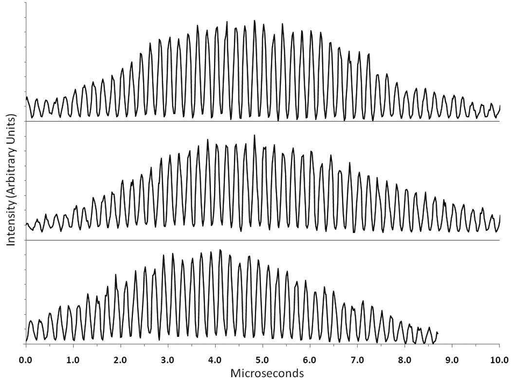
Examples of modulated waveforms detected for single particles using the digital system (y-axis is in arbitrary intensity units and individual traces are offset for clarity). The top trace is the 90° scatter signal for a single non-fluorescent bead, the middle trace is the fluorescence signal for a single Flow-Check™ bead and the bottom trace is the fluorescence signal for a single CHO cell stained with ethidium bromide.

The bypass of all analog phase shifting and filtering components makes the digital system appealing for a low-cost, user-friendly and compact lifetime system (recall Figure 3). One of the major benefits of this system is elimination of analog calibration procedures. Such procedures ‘zero’ the phase-shifts that are a result of inherent instrument delay and Rayleigh scattering signals. For example, the analog PSFC system is calibrated by first measuring the phase-response of side scatter signals using polystyrene microspheres (Duke Scientific, Inc.., 3.09 µm diameter). The detected mixed signals Q_mix (sinφ) and I_mix (cosφ) are observed on an oscilloscope, and Q_mix is minimized by adjusting the phase (Allen Avionics Inc., delay line model VAR256) to match the reference phase. A zero degree phase-shifted signal (Q_mix or sinφ = 0) effectively sets a zero lifetime. A second sample with a known lifetime is then measured to provide a calibration point so the arbitrary channel numbers from the data system can be converted into actual lifetime values. Once the calibration is established, the PMT high voltage is recorded and kept constant throughout all subsequent fluorescence measurements. Alternatively, the digital PSFC calibration simply involves measuring the phase of fluorescence beads with a known lifetime in order to provide an absolute lifetime measurement. No physical delay adjustment is necessary; the resulting phase-shift between the scatter and fluorescence signals of a bead standard are digitally recorded and used to fix the x-axis lifetime scale for subsequent fluorescence events. Any added phase delays due to the photoelectric path from the detector to the data system is cancelled out as long as all gain, triggering, and frequency settings remain the same.

2.3 Simulation procedures

In order to verify the abilities of the data system to perform lifetime analysis and sorting, modulated-Gaussian waveforms were generated with simulated phase-shifts and introduced to the data system prior to capturing real experimental data. The artificially generated data included a combination of different pulse widths, modulation frequencies, and varying modulation cycles in order to assess the digital signal processing limits of ORCAS. Table 1 outlines the various combinations measured during the simulations. A dual-channel digital function generator provided independent sinusoidal reference waveforms (at 2.5, 5, 10, and 16.667 MHz) to be mixed with two different Gaussian pulses with peak amplitudes ranging from 1 to 4 V. One of the Gaussian pulses was mixed with a continuous sine wave with an in-house signal simulator-mixing box with offset and amplitude control in order to simulate the ‘fluorescence’ modulated Gaussian. A second Gaussian and sine wave were mixed with a NIM module signal simulator-mixer in order to simulate ‘side-scatter’ modulated Gaussian pulses. Eleven a priori phase values of the high frequency waveforms were set using the function generator, from 0.5 to 25 nanoseconds. Gaussian pulses were generated having pulse widths of 2, 4, 6, 10, or 15 µs and a variety of total modulation cycles were assessed. The simulated fluorescence and side scatter pulses were measured at the four frequencies listed above and using all combinations of pulse widths, cycle number, and phase-shifts to get a comprehensive analysis of the capabilities of ORCAS for real-time lifetime analysis.

Table 1.

Overview of the simulation studies completed to test the robustness of the on-line digital lifetime measurement.

	Simulated phase delay (ns)
Frequency (MHz)	0	0.5	1	2	4	6	8	10	12	16	20	25
2.5	Measured the phase delays at 2, 6, and 15, µs pulse widths using 4, 10, and 12 modulation cycles for each respective pulse width.
5	Measured the phase delays at 2, 6, and 15 µs pulse widths using 5, 15, and 20 modulation cycles respectively.
10	Measured the phase delays at 2, 4, 6, 10, and 15 µs pulse widths and at 10, 20, and 30 modulation cycles for each pulse width.
16.667	Measured the phase delays at 2, 6, and 15 µs pulse widths using 5, 20, and 30 modulation cycles, respectively.

2.4 Lifetime-based sorting

In order to implement sorting, minor modifications to the digital data system described above were implemented. A commercial sorter (Beckton Dickinson, Inc., FACS Vantage) was retrofitted with the digital sorting system. Figure 5 is an illustration depicting the minor changes necessary for implementation on the FACS Vantage. First, a digital function generator was used to modulate a solid-state laser, which was aligned within the optical path of the commercial system. The laser used in our experiments was a 405-nm 50 mW laser (Coherent Lasers, Inc., CUBE™ model, beam diameter ~1.4mm). Secondly, high-speed preamplifiers were retrofitted onto the PMT outputs; the custom preamps are necessary to properly amplify the MHz RF signals that result from frequency-domain side-scatter and fluorescence measurements. The preamplifiers were connected directly between the PMT outputs and the ORCAS data system inputs. At this stage ORCAS was poised to directly capture and analyze the modulated signals from the PMTs. The final modification to the FACS Vantage was the introduction of two analog output signals generated by ORCAS. The synthetic signals were fed directly into the FACS Vantage data system in order to deceive the commercial system into believing it is handling two true optical inputs. Two analog output cables (from ORCAS) intercepted (via BNC connectors) the point at which the preamp board routinely connects to the data system on the FACS Vantage. This allowed the amplified signals from the optical detectors to be replaced with synthetic signals from ORCAS. By not interfering with the commercial data system, our method is versatile and flexible for use with essentially any commercial system. Even with a sorting instrument that is of the newer “digital” cytometry generation, there are no adaptations or limitations of this lifetime method. All hardware changes and retrofitting occur upstream from the commercial system’s data system. Ultimately, the purpose of the two false analog signals, which look like typical pulses from optical detectors, was: 1) to trigger the FACS Vantage in time with the events being detected by ORCAS; and 2) to adjust the FACS Vantage sort gates on the synthetic signals, which are directly correlated to the fluorescence lifetime events that are gated for sorting in TRAViS. One major constraint using this “false sorting” approach is the need to precisely time the sorting delay of the commercial system with the signals being selected for sorting at the TRAViS interface. Therefore, the two analog signals generated were combined with a programmable yet precise delay circuit to set the delay of the output analog signals relative to the actual fluorescence and scattering signal outputs from the commercial system’s PMTs. The delay must be set long enough to give the DSP time to measure the lifetime and generate a sort decision, but short enough so the particle has not reached the droplet break-off point.

Figure 5.

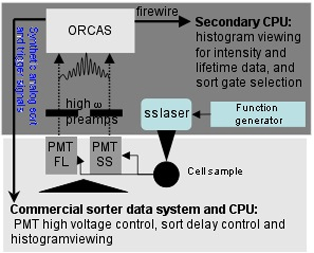
Approach to implementing digital fluorescence lifetime sorting capabilities. In this figure, the darker boxed region depicts the low-cost and compact hardware necessary to retrofit a commercial sorting system, whose components are depicted by the lighter boxed region. A solid-state laser modulated with a function generator is placed in the commercial system’s optical path. Outputs from two PMTs are routed through high bandwidth preamplifiers and sent to ORCAS. The analog outputs are fed to the commercial system’s detector input.

Ultimately, the sorting becomes a straightforward process. The commercial cytometer is set for sorting in a typical manner whereby the sort delay is observed at the FACS Vantage and adjusted by subtracting the fixed delay introduced by ORCAS. Next, the fluorescence lifetime of particles are measured at ORCAS and classified as being within a combination of three different sorting windows, using gates defined with upper and lower bounds on three single parameter histograms (e.g., light scatter, fluorescence intensity and fluorescence lifetime). Then ORCAS modifies the non-triggering analog output in real time to reflect the classification of the particles being measured. More specifically, the three gates that were set in ORCAS are used together to change the height of the analog output pulse. Eight different, equally spaced heights are generated such that the output pulse will have no height (flat) if the particle is not inside any of the three gates and maximum height if the particle is inside all 3 gates. There are 6 discrete pulse heights in between the two extremes, which correspond to other combinations of the particle being inside or outside of the three gates. More specifically, the second discrete pulse height represents particles only inside gate 1; the third, only inside gate 2; the fourth, gates 1 and 2; the fifth, gate 3; the sixth, gates 1 and 3; and the seventh, gates 2 and 3. Finally, the FACS Vantage acquires these signals and generates histograms to reveal 8 well-separated, discrete populations. At this final stage, sorting gates can be selected on one or more of the discrete populations using the standard software provided by the FACS Vantage system. Making the sort decisions with this method is truly real-time in that the decision made via the gating technique described above is done in time to generate the synthetic signals analyzed by the Vantage for the immediate sorting of the event being processed.

2.5 Cell and bead procedures

In addition to acquiring simulated digital data, stained cells and fluorescence beads were measured with the digital PSFC system for lifetime analyses. Using a cell cycle staining assay, the fluorescence lifetime of three different extrinsic nucleic acid stains intercalated into the DNA of Chinese hamster ovary (CHO) cells was measured. The cells were cultured using standard monolayer procedures in minimal essential medium (Life Technologies, Inc., alpha-MEM) containing 10% (V:V) calf serum (Hyclone, Inc., Cosmic calf serum) as described in detail previously (18). Cells were harvested in exponential growth by exposure to a trypsin solution (0.125% in calcium- and magnesium-free buffer, Life Technologies, Inc.), resuspended in complete medium, counted using an electronic particle counter (Beckman-Coulter, Inc., model Z2), centrifuged, resuspended in phosphate buffered saline (PBS) and fixed using 70% ethanol in water (18). The fixed cells were centrifuged and resuspended in PBS (10⁶ cells/mL) containing RNase (100 U/mL, Sigma Chemicals, Inc.) and either ethidium bromide (EB) (5 µg/mL), propidium iodide (PI) (1.5 µg/mL) or Syto 9 (1µM).

Fluorescence microspheres were used for calibration of lifetime values relative to the stained cell samples. Flow-Check™ (Beckman Coulter, Inc., 6 µm) microspheres were used because they excite in the same spectral region as EB and have a known singlet state lifetime of 7 ns (11). Additionally, yellow-green (3 µm and 6 µm), fluorescent yellow (7 µm) and 8-peak Rainbow microspheres (Spherotech, Inc.) were measured for lifetime values. The sorting measurements were accomplished on a mixture of fluorescence microspheres. A solution of fluorescent yellow and Flow-Check™ beads at equal concentrations (~500,000 particles/mL) was produced in distilled water. The microspheres were chosen because their easily separable lifetimes (~2 and 7 ns) cover a range that encompasses cellular autofluorescence and many common fluorophores.

3. RESULTS

3.1 Verification of digital PSFC with simulated waveforms

Using the simulated data, the lifetime values calculated by ORCAS compared favorably to the simulated phase-shifts. A cumulative study was performed that included various combinations of eleven incremental phase-shifts between the modulated-Gaussian “fluorescence” and “scatter” waveforms collected by the ORCAS system, four frequencies, six pulse widths, and eight different numbers of modulation cycles. Overall, the on-line digital Fourier transform (DFT) calculations resulted in near identical phase-shifts comparing the measured and actual values.

Table 2 provides the data characterizing ORCAS limits for measuring lifetimes at different modulation frequencies. The table displays absolute phase errors and lifetime standard deviations from synthetic data generated at pulse widths of 2, 6, and 15 µs, when a range of phase shifts (i.e. lifetimes) between the two waveforms was introduced at 2.5, 5, 10, and 16.667 MHz. Overall, a trend can be observed with standard deviation in lifetimes and modulation frequency. Specifically, the standard deviations in the lifetime values calculated digitally are systematically lower as the modulation frequency is increased, with the exception of the highest frequency, 16.667 MHz. The average cumulative standard deviations for all pulse widths were found to be 1.01, 0.74, 0.34, and 0.73 ns for 2.5, 5, 10, and 16.667 MHz, respectively. At higher frequencies the number of data points per modulation cycle is decreased, yet the number of cycles captured is generally larger and the phase-perturbation for each simulated lifetime is maximized. Thus, the deviation in the median lifetime was smallest for 10 MHz and largest at 2.5 MHz. Additionally, when the RF modulation gets close to the maximum digitization rate of the ADC (50 MS/sec), one can expect the variation in lifetime to increase, thus explaining the larger deviation at the highest measured frequency. No apparent trend with modulation frequency was seen for the absolute error between the actual phase shift and measured phase shift. In other words, for all frequency ranges measured, the DFT phase output very closely corresponded to the actual phase shift that was simulated. In fact, the lowest average and absolute error obtained was 0.014° when simulating pulses having 6 µs widths and modulating at 2.5 MHz. Overall, the absolute phase errors fell well below 0.4°, which is excellent accuracy when modulating at 10 MHz or lower frequencies. In terms of lifetime, phase perturbations of 1° at 10 MHz are equivalent to a lifetime shift of approximately 0.275 ns. Therefore, if the measured error is 0.4°, or ~0.11ns, than this digital schema can theoretically resolve lifetimes at the tenths of nanoseconds scale, as long as no other phase jitter occurs to increase the variation in the subtracted phases for the calculation of the fluorescence lifetime.

Table 2.

Error analysis results from the artificial phase shift study. The phase delays, listed at the top of the table, were simulated to imitate a phase shift that might occur between a modulated autofluorescence and modulated scattering signal due to a lifetime change. The various phase delays listed at the top of the table are in nanoseconds to provide an idea of different measurable “lifetimes.” The waveforms that were generated had 2, 6, or 15 µs pulse widths and modulation frequencies of 2.5, 5, 10, or 16.667 MHz. The values in the table are standard deviations of the lifetime (ns) calculated based on the phase shift measured digitally. The lifetime was computed using Equation 1, which assumes single exponential decay. Also in this table are absolute phase errors, noted in italics and parentheses, which are provided in units of degrees. The errors are an absolute difference between the simulated phase shift and the phase shift measured with the programmed data system.

Pulse width (µs)	Frequency (MHz)	Simulated Phase delay (ns)
		0.5	1	2	4	6	8	10	12	16	20	25
2	2.5	2.6	2.6	2.6	2.5	2.4	2.3	2.3	2.3	2.1	2	1.97
		(0.32)	(0.015)	(0.036)	(0.084)	(0.058)	(0.044)	(0.042)	(0.019)	(0.067)	(0.024)	(0.028)
	5	0.75	0.77	0.8	0.62	0.88	1.4	1.1	1.1	1.2	1.3	1.7
		(0.019)	(0.02)	(0.075)	(0.022)	(0.03)	(0.038)	(0.17)	(0.3)	(0.69)	(1.1)	(1.7)
	10	0.9	0.85	0.71	0.5	0.38	0.29	0.28	0.22	0.17	0.19	0.3
		(0.015)	(0.042)	(0.069)	(0.21)	(0.28)	(0.4)	(0.53)	(0.7)	(0.94)	(1.2)	(1.6)
	16.667	0.48	0.42	0.34	0.28	0.22	0.33	0.33	0.42	1.4	1.5	1.5
		(0.059)	(0.12)	(0.16)	(0.09)	(0.23)	(0.64)	(1)	(1.1)	(0.56)	(0.15)	(0.19)
6	2.5	0.31	1.3	0.33	0.34	0.3	0.32	0.32	0.31	0.31	1.5	0.31
		(0.0041)	(0.0046)	(0.0043)	(0.011)	(0.014)	(0.0084)	(0.0048)	(0.012)	(0.018)	(0.035)	(0.042)
	5	1	1	1	0.92	0.63	0.18	0.15	0.12	0.68	0.82	0.84
		(0.14)	(0.23)	(0.22)	(0.31)	(0.39)	(0.4)	(0.04)	(0.16)	(0.22)	(0.16)	(0.3)
	10	0.68	0.64	0.6	0.52	0.48	0.44	0.59	0.49	0.17	0.49	0.33
		(0.013)	(0.042)	(0.059)	(0.12)	(0.13)	(0.004)	(0.02)	(0.038)	(0.092)	(0.09)	(0.079)
	16.667	0.6	0.44	0.24	0.244	0.355	0.44	0.14	0.58	0.76	1	1.9
		(0.05)	(0.045)	(0.053)	(0.06)	(0.03)	(0.075)	(0.067)	(0.023)	(0.064)	(0.11)	(0.19)
15	2.5	0.23	0.23	0.22	0.21	0.2	0.19	0.18	0.18	0.18	0.17	0.16
		(0.4)	(0.003)	(0.007)	(0.004)	(0.006)	(0.006)	(0.007)	(0.033)	(0.01)	(0.01)	(0.009)
	5	0.46	0.48	0.47	0.46	0.46	0.33	0.48	0.47	0.51	0.56	0.71
		(0.14)	(0.21)	(0.24)	(0.39)	(0.43)	(0.031)	(0.029)	(0.026)	(0.07)	(0.09)	(0.18)
	10	0.37	0.36	0.32	0.26	0.22	0.18	0.14	0.12	0.11	0.18	0.38
		(0.016)	(0.032)	(0.052)	(0.1)	(0.15)	(0.21)	(0.27)	(0.33)	(0.45)	(0.59)	(0.74)
	16.667	0.47	0.42	0.34	0.26	0.26	0.31	0.4	0.55	1.3	1.5	2.1
		(0.008)	(0.0002)	(0.018)	(0.015)	(0.04)	(0.048)	(0.007)	(0.061)	(0.041)	(0.11)	(0.162)

In addition to an analysis of the modulation frequency limits at a fixed ADC resolution, we assessed how the width of the pulses captured might impact the lifetime and phase measurable by ORCAS. Again, Table 2 provides the cumulative results. Overall the lifetime standard deviations went down with increasing pulse widths at fixed modulation frequencies. For example, the average standard deviation when combining results from all frequencies was 1.12, 0.62, and 0.41 at 2, 6, and 15 µs, respectively. A smaller variation in the lifetime at the larger pulse widths is consistent with the fact that when observing a fixed number of modulation cycles, the modulation depth changes for the total number of cycles depending on the pulse width. More specifically, the AC/DC value, or amplitude over average pulse strength, is stronger for a long pulse where the Gaussian “tails” are not as apparent as for shorter pulses. The average phase errors were 0.3°, 0.1° and 0.1° for the simulated 2, 6, and 15 µs pulse widths, respectively. Similarly, it is apparent that in order to maximize the phase accuracy, one might increase the pulse width. However, it is possible to run at shorter pulse widths simply by limiting the number of modulation cycles collected. Changing the number of cycles adds flexibility that can improve or degrade the phase measurement; simply put, there is a trade-off between a weak DFT calculation and a strong modulation cycle.

Because the flexibility provided in TRAViS and ORCAS allows the user to control the number of modulation cycles used in the DFT, a simulation study was performed for differing number of cycles at a fixed frequency. Table 3 provides the absolute phase error results when comparing the number of modulation cycles at various pulse widths at a 10 MHz modulation frequency. The average phase errors for all pulse widths were found to be 0.3°, 0.3°, and 0.2° for 10, 20, and 30 total modulation cycles collected, respectively. Thus, overall low and consistent absolute phase errors were found with a small decrease in error as the number of cycles collected increased. However, the phase error at different numbers of cycles collected for a fixed pulse width changes more dramatically. For example, the DFT resulted in phase errors of 0.411°, 0.054°, 0.07° and 0.02° for 4, 6, 10, and 15 µs pulses when the number of cycles collected was changed from 10 to 30.

Table 3.

Results of the absolute phase errors measured after waveforms were generated at a single modulation frequency (10 MHz) using four different pulse widths. During acquisition, three different sets of data were taken in which the data system was directed to collect three different total modulation cycle lengths. The values populating the table are the absolute errors (degrees) between the simulated phase shift (actual value) and measured phase shift value. In the table heading, the simulated phase shift value is provided in degrees as well as in nanoseconds to relate the shift to a true lifetime value that might occur during a fluorescence measurement.

Simulated phase delay (degree, ns)
	Pulse width (µs)	3.6 , 1	7.2 , 2	14.4 , 4	21.6 , 6	28.8 , 8	36 , 10	43.2 , 12	57.6 , 16
10 cycles	4	0.12	0.15	0.15	0.07	0.23	0.09	0.17	2.7
	6	0.031	0.035	0.13	0.23	0.28	0.29	0.21	0.27
	10	0.038	0.069	0.11	0.16	0.23	0.31	0.37	0.49
	15	0.04	0.053	0.095	0.14	0.19	0.25	0.31	0.42
20 cycles	4	0.011	0.005	0.09	0.034	3.7	0.09	0.26	0.7
	6	0.044	0.026	0.13	0.17	0.24	0.29	0.41	0.58
	10	0.023	0.052	0.092	0.14	0.19	0.24	0.3	0.43
	15	0.022	0.04	0.073	0.14	0.18	0.24	0.3	0.4
30 cycles	4	0.045	0.05	0.051	0.04	0.046	0.05	0.052	0.053
	6	0.016	0.053	0.11	0.18	0.25	0.33	0.41	0.56
	10	0.022	0.034	0.07	0.12	0.17	0.22	0.18	0.4
	15	0.032	0.052	0.1	0.15	0.21	0.27	0.33	0.5

3.2 Comparison of analog to digital PSFC using experimental data

Figure 6 and Table 4 provide experimental results obtained by simultaneous digital and analog PSFC. The lifetime measurements were acquired at 6.125 MHz modulation frequency using the PSFC fluidics (approximately 15 µs transit times) with fluorescence and side-scatter PMTs and exciting with the argon laser at 488 nm. By splitting the PMT outputs we were able to take measurements synchronously with the digital and analog systems. Table 4 provides the geometric mean and standard deviations of all microsphere and stained-cell samples. The absolute lifetimes measured were similar; for example, the lifetime of propidium iodide intercalated into the DNA of fixed cells was found to be 15.3 ± 0.9 ns when measured with the analog PSFC system, while an average lifetime of 15.6 ± 1.9 ns was obtained when digital acquisition and DFT analysis was used. The bead and stained-cell measurements were repeated; new cell samples were prepared as well as new solutions of fluorescent microspheres. Similar average lifetimes and standard deviations in the lifetime measurement were acquired for the repeated experiments.

Figure 6.

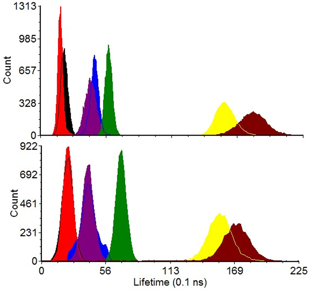
Lifetime results from cell and fluorescence microspheres acquired on an analog (A) and digital (B) version of the PSFC system. The black, red, blue, purple, green, yellow, and maroon histograms represent lifetime results for 2 µm yellow-green microspheres, 6 µm yellow-green microspheres, 8-peak Spherotech™ rainbow microspheres, Syto9-stained CHO cells, Flow-Check™ microspheres, propidium iodide-stained CHO cells, and ethidium bromide-stained CHO cells, respectively.

Table 4.

The resulting lifetime values (ns) and standard deviations (ns) from experimental data acquired with the digital and analog PSFC systems.

Sample	Lifetime Digital	Std Dev Digital	Lifetime Analog	Std Dev Analog
2 mm yellow-green microspheres	2.3	0.49	2.44	0.28
6 mm yellow-green microspheres	2.3	0.47	2.15	0.23
Syto9 stained CHO cells	4.1	0.5	4.56	0.46
Spherotech 8-peak Rainbow microspheres	3.9	1.3	4.82	0.57
Flow-check™ microspheres	6.9	0.46	7.0	0.31
Propidium iodide stained CHO cells	15.6	1.9	15.3	0.93
Ethidium bromide stained CHO cells	17	2.1	17.38	1.56

3.4. Lifetime sorting results

The sorting experimental results are provided in Figure 7. The system was adjusted to give a droplet delay of 20 drops at 35.2 KHz (567 µs). The delay through ORCAS was set to be 12 drops (340 µs) and the software on the Vantage was used to set a sort delay of 8 drops (227 µs) so the total sort delay would be correct. The actual “dead time” of the system was thus equivalent to 8 droplets on the Vantage (227 µs). The sort delay was verified normally. Recall, up to eight discrete populations are generated based on events being in a combination of three gate selections made with TRAViS. In this work, the three gate selections made at the data system were: 1) gating around the lower lifetime bead population, which overlapped with 2% of the longer lifetime bead population; 2) gating around both bead populations based on their peak fluorescence intensity values; and 3) gating around both bead populations based on their peak side scattering signals. Then, in order to sort based on fluorescence lifetime, it was necessary to determine which of the discrete populations generated shall be selected for the sort decision via the FACS Vantage computer interface. The maximum population whereby events within all 3 gates set in TRAViS was ultimately selected for sorting. Figure 7A shows the fluorescence lifetime histogram with the first of the three gates set in TRAViS, encompassing the beads with the lower lifetime. Because the two bead populations had an approximate lifetime difference of 4–5 ns, the ORCAS digital lifetime system was easily resolved the two populations. Triggering was performed at an unused FACS Vantage channel input, and the analysis rate was adjusted to get a sort rate of ~330 particles/second.

Figure 7.

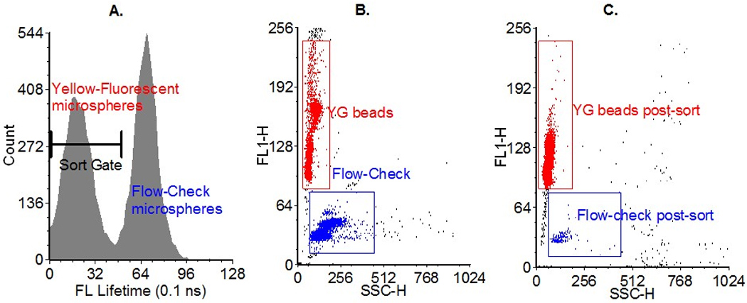
A) Fluorescence lifetime histogram acquired with the digital lifetime data system. One of the three gates adjusted in TRAViS is displayed and positioned such that the bead population with the shorter lifetime was selected. B) Dot plot of the initial bead mixture, showing an approximately equal mixture of yellow-green (red gate) and Flow-Check™ microspheres (blue gate). The red gate includes 42% of all events detected and the blue gate includes 54% of all events detected. C) Dot plot of the post-sorted mixture. The red gate includes 96% of all events detected and the blue gate includes 1.6% of all events detected, which resulted in a purity of sort of approximately 98%.

Also in Figure 7 are the final sort purity results taken on the FACS Vantage system without the digital lifetime components. Cytometric analysis was performed with the same laser used for sorting and with the normal FACS Vantage preamplifiers, detectors, and data system. Figure 7B shows a dot plot representing the bead mixture (side scatter vs. fluorescence intensity) before sorting. Prior to sorting, approximately 50% of the events collected are made up of the Flow-check™ microspheres and likewise, the other half represents the yellow-green beads. After sorting, analysis was performed again to determine the sorting efficiency based on the fluorescence lifetime. A sort purity of 98.3% was achieved based on reanalysis of ~500,000 sorted beads. The actual sort purity was probably higher, since the lifetime sort window was set such that a small fraction of the beads with the higher lifetime were included in the sort region.

4. DISCUSSION

A digital phase sensitive flow cytometer that utilizes ORCAS (17) for analysis and sorting has been described and validated for lifetime measurements at select modulation frequencies. The digital system performs comparable to the analog system and has the benefit of being a compact and inexpensive means of obtaining fluorescence lifetime on commercial flow cytometers. With the addition of a function generator and direct modulation of a solid-state laser, frequency-domain cytometry measurements can be easily adapted on a commercial sorting system. Using appropriate PMT preamplifiers (extended bandwidth), a flexible data acquisition system, and Fourier signal processing, the average lifetime of a fluorophore is obtainable in real time.

Although this work demonstrates the ability to obtain lifetime values as robustly as previously optimized analog systems, users should be aware of the limitations of lifetime measurements in general. As with any cytometer, Poisson statistics dictates the variation in photoelectrons produced by a PMT. The variation can be large when fluorescence signals are low and background is high. The new digital lifetime approach handles the dim signals directly as opposed to collecting the signals, amplifying them further, mixing them and sending them through ratio modules. Therefore, the digital lifetime method eliminates several other possible sources of noise. However, in any frequency-domain spectroscopic measurement the occurrence of low modulation depth, which is often a product of dim signals, affects the lifetime value. Thus, an optimized modulated excitation signal will provide the best results. It is noteworthy to add that as with any cytometric assay, it is important to control all variables to eliminate any factors that may affect the lifetime value. For example, the modulation frequency, PMT gain, offset values, threshold value, and the number of cycles detected, should stay the same for all experiments for the Fourier analysis to be most accurate.

With simulated data, we demonstrated that accurate lifetime measurements are possible over a wide range of pulse widths and frequencies, but there still are a number of areas where digital PSFC can be enhanced. The ability to resolve an accurate phase at a given event width and modulation frequency is largely dependent on the sample rates that are supported by ORCAS. Owing to the 50 MS/sec commercial ADC, event widths of 2 to 15 µs at the base of the generated pulse (modulating at 2.5 to 16.667 MHz) provided sufficient sample sizes to resolve lifetime with error as low as hundredths of nanoseconds. For example, if a lifetime on the order of 4 ns were to be measured with a 10 MHz modulation frequency, it would be beneficial to capture more modulation cycles for the Fourier analysis, as illustrated in Table 3. If the pulse width is 4 µs and cannot be adjusted due to limitations of the laser spot, particle size or flow rate, then capturing 30 cycles of the modulated waveform (as opposed to only 10 cycles) would reduce the error by 0.1 degree. Equating this value directly to time (not accounting for the relationship of phase to lifetime via Equation 1) is 0.027 ns, which can perpetuate large CVs that are due to the analysis as opposed to true variations in the lifetime of the fluorophore being detected. Also, at higher frequencies one can expect that this accuracy will decline unless there is an increase in ADC resolution. The low radio-frequency ranges studied herein are adequate for measurement of lifetime values that range as short as 1 nanosecond up to tens of nanoseconds.

For sorting of particles based on lifetime, the sorting rate of ~330 particles/second we achieved will be useful for many applications but may be limiting for high-throughput applications. There is a significant dead time in the system (hundreds of microseconds), which is caused by several factors. Having only one DSP to capture and process the waveforms from multiple detectors does not allow parallel processing of the captured waveforms. The processing required to perform the DFT calculations is significantly more than simple peak, width and area measurements. The hardware that generates the synthetic signals for the cytometer was not designed for high throughput analysis and therefore does not allow the sort decisions to be buffered. This effectively creates a dead time that is somewhat longer than the delay from the interrogation point to the droplet break-off point. This presents a problem because all events that are detected while a previous lifetime measurement is being processed are simply ignored and thus lost. Moving the pre-processing of the captured waveforms into the field-programmable gate array (FPGA) will reduce the amount of data that must be sent to and processed by the DSP by an order of magnitude, while at the same time removing some of the calculations entirely. Redesigning the hardware that generates the synthetic signals to allow sort decisions to be buffered would eliminate the dead time caused by this current limitation. The combination of these two improvements should greatly increase the sorting throughput of the system.

The results presented using a digital approach provide an overall promising outlook for lifetime measurements in flow cytometry. Prior lifetime acquisition with the analog system required a “zero lifetime” to be established for non-fluorescent samples. Yet with the digital system, there is no real “zero lifetime” value. Therefore calibration simply becomes measuring a known lifetime standard and comparing that to the unknown sample. The most appealing aspect of the digital system is its simplicity: little modulation hardware is required and, when coupled with a rapid fitting routine, lifetime can be calculated on-line at essentially instantaneous speeds. The only hardware and software requirements for digital lifetime acquisition are a signal generator, high-frequency preamplifiers, a data acquisition system that captures correlated waveforms, and a fitting routine. With the aforementioned components, this method is applicable for any cytometer because the frequency domain hardware and software are independent of the data acquisition system of the commercial instrument. Although not necessary with solid-state lasers, an external modulator may be used. A more optimized form of the digital system we are investigating uses ORCAS to generate the modulation signals, which would eliminate the need to have reference signals split from a secondary frequency synthesizer. Rather, the internal ORCAS clock generating the modulation frequency would be used to set the reference phase relative to all the detected modulated-Gaussian pulses. With such a system, only a solid-state laser, some high-speed preamps, and the ORCAS data system would be required to add lifetime to an existing instrument. Additionally, one might envision the use of advanced multi-frequency systems with solid-state lasers and DSP programming. Exploiting multiple frequencies produced with on-off modulation and Fourier analysis to reveal multiple harmonics is one method of introducing advanced frequency domain methods. Multi-frequency measurements will enable the real-time analysis of multiple lifetimes for one particle. The acquisition of multi-decay kinetics is a very promising technique that will allow the user to multiplex based on the lifetime using only one detector. We are also expanding the digital technology to enable multi-frequency measurements. Ultimately, as the cytometry user community continues to grow it is important for technologies to become user-friendly and to expand specialized cytometry capabilities commercially. This digital approach to average lifetime cytometry measurements is a technology that has great potential for this commercial translation.

REFERENCES

- 1.Pinsky BG, Ladasky JJ, Lakowicz JR, Berndt K, Hoffman RA. Phase-resolved fluorescence lifetime measurements for flow cytometry. Cytometry. 1993;14(2):123–135. doi: 10.1002/cyto.990140204. [DOI] [PubMed] [Google Scholar]
- 2.Steinkamp JA, Crissman HA. Resolution of fluorescence signals from cells labeled with fluorochromes having different lifetimes by phase-sensitive flow cytometry. Cytometry. 1993;14(2):210–216. doi: 10.1002/cyto.990140214. [DOI] [PubMed] [Google Scholar]
- 3.Steinkamp JA, Yoshida TM, Martin JC. Flow cytometer for resolving signals from heterogeneous fluorescence emissions and quantifying lifetime in fluorchrome-labeled cells/particles by phase-sensitive detection. Review of Scientific Instruments. 1993;64(12):3440–3450. [Google Scholar]
- 4.Deka C, Lehnert BE, Lehnert NM, Jones GM, Sklar LA, Steinkamp JA. Analysis of fluorescence lifetime and quenching of FITC-conjugated antibodies on cells by phase-sensitive flow cytometry. Cytometry. 1996;25(3):271–279. doi: 10.1002/(SICI)1097-0320(19961101)25:3<271::AID-CYTO8>3.0.CO;2-I. [DOI] [PubMed] [Google Scholar]
- 5.Sailer BL, Steinkamp JA, Crissman HA. Flow cytometric fluorescence lifetime analysis of DNA-binding probes. Eur J Histochem. 1998;42 Spec No: 19-27. [PubMed] [Google Scholar]
- 6.Cui HH, Valdez JG, Steinkamp JA, Crissman HA. Fluorescence lifetime-based discrimination and quantification of cellular DNA and RNA with phase-sensitive flow cytometry. Cytometry A. 2003;52A(1):46–55. doi: 10.1002/cyto.a.10022. [DOI] [PubMed] [Google Scholar]
- 7.Sailer BL, Valdez JG, Steinkamp JA, Crissman HA. Apoptosis induced with different cycle-perturbing agents produces differential changes in the fluorescence lifetime of DNA-bound ethidium bromide. Cytometry. 1998;31(3):208–216. [PubMed] [Google Scholar]
- 8.Sailer BL, Nastasi AJ, Valdez JG, Steinkamp JA, Crissman HA. Differential effects of deuterium oxide on the fluorescence lifetimes and intensities of dyes with different modes of binding to DNA. J Histochem Cytochem. 1997;45(2):165–175. doi: 10.1177/002215549704500203. [DOI] [PubMed] [Google Scholar]
- 9.Sailer BL, Nastasi AJ, Valdez JG, Steinkamp JA, Crissman HA. Interactions of intercalating fluorochromes with DNA analyzed by conventional and fluorescence lifetime flow cytometry utilizing deuterium oxide. Cytometry. 1996;25(2):164–172. doi: 10.1002/(SICI)1097-0320(19961001)25:2<164::AID-CYTO5>3.0.CO;2-H. [DOI] [PubMed] [Google Scholar]
- 10.Keij JF, Steinkamp JA. Flow cytometric characterization and classification of multiple dual-color fluorescent microspheres using fluorescence lifetime. Cytometry. 1998;33(3):318–323. [PubMed] [Google Scholar]
- 11.Steinkamp JA, Keij JF. Fluorescence intnsity and lifetime measurement of free and particle-bound fluorophore in a sample stream by phase-sensitive flow cytometry. Review of Scientific Instruments. 1999;70(12):4682–4688. [Google Scholar]
- 12.Deka C, Steinkamp JA. Time-resolved fluorescence-decay measurement and analysis on single cells by flow cytometry. Applied Optics. 1996;35(22):4481–4489. doi: 10.1364/AO.35.004481. [DOI] [PubMed] [Google Scholar]
- 13.Steinkamp JA, Parson JD. Flow cytometric, time-resolved measurements by frequency heterodyning of fluorescence emission signals. Proceedings of the SPIE-The International Society for Optical Engineering. 2001;4260:166–174. [Google Scholar]
- 14.Deka C, Cram LS, Habbersett R, Martin JC, Sklar LA, Steinkamp JA. Simultaneous dual-frequency phase-sensitive flow cytometric measurements for rapid identification of heterogeneous fluorescence decays in fluorochrome-labeled cells and particles. Cytometry. 1995;21(4):318–328. doi: 10.1002/cyto.990210403. [DOI] [PubMed] [Google Scholar]
- 15.Parson JD, Deka C, Habbersett R, Martin JC, Naivar MA, Steinkamp JA, Wilder ME, Jett JH. Digital porcessing of phase sensitive flow cytometry signals. Cytometry Suppl. 1994;7(74) [Google Scholar]
- 16.Beisker W, Klocke A. Fluorescence lifetime meaurements in flow cytometry. Proceedings of the SPIE-The International Society for Optical Engineering. 1997;2982:436–445. [Google Scholar]
- 17.Naivar MA, Parson JD, Wilder ME, Habbersett RC, Edwards BS, Sklar L, Nolan JP, Graves SW, Martin JC, Jett JH, Freyer JP. Open, reconfigurable cytometric acquisition system: ORCAS. Cytometry A. 2007;71A(11):915–924. doi: 10.1002/cyto.a.20445. [DOI] [PubMed] [Google Scholar]
- 18.LaRue KEA, Kahlil M, Freyer JP. Microenvironmental regulation of proliferation in EMT6 multicellular spheroids is mediated through differential expression of cyclin-dependent kinase inhibitors. Cancer Res. 2004;64(5):1621–1631. doi: 10.1158/0008-5472.can-2902-2. [DOI] [PubMed] [Google Scholar]