Construction of Confidence Regions for Isotopic Abundance Patterns in LC/MS Data Sets for Rigorous Determination of Molecular Formulas

Abstract

It has long been recognized that estimates of isotopic abundance patterns may be instrumental in identifying the many unknown compounds encountered when conducting untargeted metabolic profiling using liquid chromatography/mass spectrometry. While numerous methods have been developed for assigning heuristic scores to rank the degree of fit of the observed abundance patterns with theoretical ones, little work has been done to quantify the errors that are associated with the measurements made. Thus, it is generally not possible to determine, in a statistically meaningful manner, whether a given chemical formula would likely be capable of producing the observed data. In this paper, we present a method for constructing confidence regions for the isotopic abundance patterns based on the fundamental distribution of the ion arrivals. Moreover, we develop a method for doing so that makes use of the information pooled together from the measurements obtained across an entire chromatographic peak, as well as from any adducts, dimers, and fragments observed in the mass spectra. This greatly increases the statistical power, thus enabling the analyst to rule out a potentially much larger number of candidate formulas while explicitly guarding against false positives. In practice, small departures from the model assumptions are possible due to detector saturation and interferences between adjacent isotopologues. While these factors form impediments to statistical rigor, they can to a large extent be overcome by restricting the analysis to moderate ion counts and by applying robust statistical methods. Using real metabolic data, we demonstrate that the method is capable of reducing the number of candidate formulas by a substantial amount, even when no bromine or chlorine atoms are present. We argue that further developments in our ability to characterize the data mathematically could enable much more powerful statistical analyses.

Metabolomics(1) is a powerful tool for investigating biological systems through the study of biofluids such as plasma or urine. Samples are typically analyzed using either nuclear magnetic resonance (NMR) or mass spectrometry (MS). When the latter platform is used, it is often preceded by either liquid or gas chromatography, resulting in the combined techniques LC/MS and GC/MS, respectively.(2) Metabolic samples are highly complex mixtures that are comprised of thousands of compounds. Because of the high sensitivity of the LC/MS and GC/MS platforms, experimental runs will typically produce a very large number of signals, which are induced by unknown metabolites whose identification forms a core part of the analysis. Consequently, a central challenge in MS-based metabolomics lies in developing efficient methods for reliably identifying the chemical structures of metabolites on the basis of the information contained in mass spectral data.

The primary measure that is used to identify unknown compounds is their estimated masses, which, under optimal conditions, may be accurate to within a few parts per million for modern time-of-flight mass spectrometers.(3) Fourier transform ion cyclotron resonance (FTICR) mass spectrometers are capable of sub 1 ppm accuracy,(4) but can be prohibitively expensive. Compounds may also be identified on the basis of their chromatographic elution times; however, this measure is instrument-specific and typically has rather poor reproducibility.

It is often possible to unambiguously identify unknowns at very low masses (<100 Da) using only the mass estimate. However, the number of possible chemical formulas and structures increases dramatically with mass, resulting in a very large number of “candidate formulas”. Many “chemically unrealistic” formulas may be discarded using various heuristic rules based on the ratios of elements involved as well as their valences.(5) Nevertheless, this will often leave a substantial number of viable candidate formulas, especially if the experiment is carried out on a mass spectrometer with limited mass accuracy.(6)

Further constraints can be placed on the possible formulas of unknown metabolites by making use of their fragmentation patterns.(7) Unlike mass estimates, the observed fragmentation patterns may reveal information regarding the structure of the metabolite and thereby enable the analyst to distinguish between isomers. However, their analysis can be severely confounded if there is close coelution of distinct metabolites, whose fragments must be distinguished. While improved chromatographic techniques such as Ultra-Performance Liquid Chromatography(8) (UPLC) have helped to alleviate this problem, the partial coelution of distinct metabolites remains a routine phenomenon in LC/MS experiments. Various statistical techniques are available to help identify related parent−fragment pairs.⁹⁻¹¹

It is also possible to identify a metabolite by means of its observed isotopic abundance pattern. This measure is especially useful for detecting the presence of bromine or chlorine due to the highly characteristic isotopic distributions of those atoms, but even for compounds comprised solely of the most biologically abundant elements, it provides information that can be crucial for effective formula identification. An insightful study by Kind and Fiehn(12) demonstrated that if a hypothetical mass spectrometer with an accuracy of 0.1 ppm were available, it would be less successful at identifying unknowns than a mass spectrometer capable of only 3 ppm accuracy, but which was also capable of estimating isotopic ratios with a fixed accuracy of 2%. This would suggest that the extensive efforts put into improving the mass accuracy of mass spectrometers might be somewhat misplaced if good estimates of isotopic abundance patterns could be obtained instead.

Since all mass spectrometers produce errors in their spectral intensity measurements, a fundamental question that must be asked when exploiting isotopic abundance patterns is whether the deviation of a given theoretical isotopic abundance pattern from the observed abundance pattern is sufficiently small that it may realistically be attributed to the measurement error. If not, then the chemical formula to which the theoretical isotopic abundance pattern corresponds may be deemed to be inconsistent with the observed data and excluded from the list of candidate formulas. However, rather than addressing this question, most available methods attempt only to rank the degree of fit of all the feasible molecular formulas by means of various heuristic scores.¹³⁻¹⁵ Other procedures simply assume that the observed isotopic ratios are accurate to within a few percent,(12) but this is somewhat imprecise, as the accuracy depends on numerous factors, including the spectral intensity and the type of detector system used.

Therefore, while these heuristic methods can be extremely useful analytical tools, they do not enable the analyst to quantify, in a statistically meaningful manner, the range of molecular formulas that could realistically have produced the observed isotopic abundance pattern. The preferred method for doing so, according to classical frequentist statistical theory, would be through the construction of a confidence region which, by definition, would cover the true parameter values, say, 95% of the time. However, the construction of such intervals requires a detailed understanding of the fundamental distribution of the data, which will in turn be dependent on the type of mass spectrometer used as well as the forms of preprocessing that are applied to the data.

In the following we demonstrate that the construction of conservative confidence regions is in fact possible and has the potential to reduce the number of candidate formulas for unknown metabolites by a substantial amount, even when the latter do not contain bromine or chlorine. Moreover, we show how the isotopic abundance patterns observed at distinct chromatographic scans and at distinct fragments, adducts, and polymers that are derived from the same underlying metabolite may be pooled to place further constraints on its identity. The statistical model from which the procedure is derived is tailored to the type of data produced by time-of-flight mass spectrometers employing a time-to-digital converter (TDC) as part of their detector systems. It is therefore not expected to be applicable to different types of mass spectrometers, such as FTICR, or to time-of-flight mass spectrometers employing the alternative analog-to-digital converters (ADCs), although similar techniques might be developed for such instruments.

Theory

Background

In general, the nature of LC/MS metabolic data is extremely complex. This is in part due to the inherent complexity of metabolic samples, but it is also due to the sophisticated nature of the analytical platform itself. Moreover, while widely used preprocessing procedures such as peak alignment and normalization may serve to facilitate a qualitative analysis, they typically render the underlying statistical distribution of the data far more complex. Nevertheless, some of the elementary characteristics of the truly raw data can be described by means of rather simple mathematical models.

A fundamental feature of time-of-flight mass spectrometry is that the rate of ion arrivals at the detector plate is governed by the Poisson distribution.(16) However, the distribution of the recorded data is generally rather more complicated and, as mentioned above, depends on the type of detection system employed. Many mass spectrometers make use of TDCs to record the timing and number of ion arrivals. An important advantage of TDCs is that they are effectively able to block out electronic noise,(17) a feature which can, to some extent, enable them to preserve the Poisson distribution of the data. However, each ion arrival triggers a period of “dead time” during which the TDC is incapable of registering further ion arrivals. Thus, when the rate of the ion arrivals is high, the data output will display strong deviations from the Poisson distribution, although these can be reduced somewhat by applying statistical correction methods to the data.(18)

In principle, a comprehensive mathematical model of a TDC-based detector system might be capable of accounting for this limitation. However, the construction of such a model would require very extensive knowledge of the workings of the TDC as well as of the dynamics of the ionization process and the various ion-focusing mechanisms, which determine the shapes of the mass peaks. In the following analysis we will therefore focus on the scenario where ion counts are moderate so that the Poisson approximation works well. Thus, on the basis of the assumption that the data are Poisson-distributed, a statistically rigorous method for determining whether a given chemical formula is consistent with the observed isotopic abundance pattern is presented in the following subsection.

Statistical Model

In the following we will work with the centroided mass peaks. This does not distort the Poisson nature of the data as the sum of independent Poisson-distributed variables is itself Poisson-distributed. It will be assumed that the peaks studied are comprised of only one metabolite, which may be referred to as M. Let us suppose that there are s + 1 isotopologues of M, so that we may refer to them as M₀, M₁, ..., M_s.

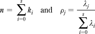
According to the Poisson distribution, the probability of obtaining the count k_i for the isotopologue M_i is given by

where the parameter λ_i denotes the mean number of ion arrivals of the ith isotopologue, M_i, within one chromatographic scan. Consequently, the probability of obtaining the sequence of counts k₀, k₁, ..., k_s from the full set of isotopologues can be written as

Each λ_i in the above expression governs the absolute number of ion arrivals of the corresponding isotopologue, so that a total of s + 1 parameters are required. However, when investigating isotopic abundance patterns, we are interested in the relative, rather than the absolute, numbers of ion arrivals. We may therefore work with the distribution of the ion counts at the various isotopologues, conditional on the total number of ion arrivals. If

then the conditional distribution that we seek may be written as

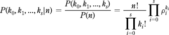which is a multinomial distribution with n trials and probabilities ρ₀, ρ₁, ..., ρ_s where ρ_i is the isotopic abundance of M_i.

Confidence Regions

Confidence regions may be constructed by exploiting the fundamental duality between tests of hypotheses and confidence regions, whereby the confidence region is defined as the set of parameter values that are not rejected by the corresponding test of hypothesis. Several methods are available for constructing confidence regions around multinomial proportions, and while no one method is universally accepted as being optimal in all circumstances, the one based on Pearson’s χ² test is arguably an uncontroversial choice. The statistic, which in this case must be “inverted”, can be written as

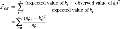where the p_i indicate the multinomial parameters that are being tested. If, for all i, p_i = ρ_i, then x²_(M) approximates the χ² distribution with s degrees of freedom (χ²_s in the following). Thus, given the counts k₀, k₁, ..., k_s, a 95% confidence region can be defined as the set of p_i for which x²_(M) is less than or equal to the 95th percentile of the χ²_s distribution. Since this procedure may be unreliable when the counts are very low, a standard rule is to require np_i ≥ 5 for all i. Chromatographic scans for which this condition is not met can be pooled together, as will be shown below.

Note that owing to the dependence between the p_i, the confidence region defined above cannot be expressed as a set of intervals around each of the estimated probabilities. Rather the shape of the confidence region is ellipsoidal, which can make its interpretation rather awkward, depending on the physical nature of the multinomial probabilities. A number of procedures have been developed for constructing “simultaneous confidence intervals” which can be expressed as a simple set of intervals around each of the estimated probabilities.(19) However, while this can indeed facilitate the interpretation, it also makes the resulting confidence region larger than it needs to be, reducing the statistical power of the test. Moreover, when the purpose of the study is formula elucidation, where there are a finite number of possible multinomial probabilities and the aim is simply to narrow them down as far as possible, any extension of the confidence region seems difficult to justify.

We therefore propose that the most appropriate method for constructing confidence regions for isotopic abundance patterns is the one based directly on the ellipsoid described above. In practice, this will entail conducting a test of hypothesis based on the x²_(M) statistic for all chemically realistic formulas that are consistent with the observed mass estimate. The x²_(M) statistics must be calculated using the multinomial probabilities that correspond to the known isotopic abundance patterns of the candidate formulas. While the total number of formulas for which the statistic must be calculated may be large, depending on the mass accuracy, each individual calculation requires very little computational power.

Pooling Information

It has long been understood that improved estimates of both masses and isotopic abundance patterns may be obtained by combining the measurements obtained across a compound’s chromatographic peak. However, the procedure by which the data are pooled must be chosen carefully if a valid confidence region is to be constructed for the combined data set. Moreover, to make full use of the information in the acquired data set, the pooling procedure should ideally be generalized to incorporate the observed isotopic abundance patterns of any adducts, fragments, or dimers of the compound of interest.

Since the power of Pearson’s χ² test increases with the sample size, a higher value of n will reduce the volume of the confidence region and allow us to exclude a larger number of chemical formulas. However, owing to the risk of detector saturation, we cannot apply the test to scans with high counts, as these generally do not adhere to the Poisson distribution. Fortunately there are a number of ways of reducing the volume of the confidence region without using high counts.

The χ² distribution has the very useful property that if the statistic X adheres to the χ²_A distribution and the statistic Y adheres to the χ²_B distribution, then X + Y adheres to the χ²_A+B distribution. We may therefore calculate the x²_(M) statistic for each of the chromatographic scans, obtained from the metabolite M, and sum the resulting x²_(M) statistics to obtain a pooled statistic, X²_(M). If we have a total of N_(M)x²_(M) statistics, then X²_(M) approximates the χ² distribution with N_(M)s degrees of freedom, under the null hypothesis that the multinomial probabilities p₀, p₁, ..., p_s used in calculating x² reflect the true isotopic abundance pattern of M. Chromatographic scans for which at least one isotopologue produces counts that are high enough to induce substantial detector saturation should be left out. The more counts pooled in this manner, the greater the power of the test, so this is a rare scenario in which broader chromatographic peaks are desirable, although, of course, this is entirely dependent on them not having any overlap with other peaks.

There is in fact a rather more straightforward way to pool the data. The multinomial interpretation of the ion counts of the isotopologues applies to all of the scans that comprise a chromatographic peak. These multinomials differ in the number of trials, n, but they all share the same probabilities, which are governed by the same isotopic abundance pattern. Therefore, the counts derived from each isotopologue may simply be summed, reducing the entire data set to the outcome of a single multinomial distribution with a potentially very large number of trials. While this method of pooling the data is simpler and has greater statistical power than the one based on summing the x²_(M) statistics, the latter method has the advantage of being capable of providing a p-value associated with each scan. As will be shown below this turns out to be very useful when constructing confidence regions that are robust to small departures from the model assumptions, as are often encountered in practice.

It is possible to further constrain the confidence region by exploiting the information that is contained in the isotopic abundance patterns of “derivatives” of the compound being investigated, such as adducts, fragments, and polymers, which are frequently observed in LC/MS experiments. Consider a derivative D which has been definitively identified in this manner and which has the isotopologues D₀, D₁, ..., D_t. As with the underlying metabolite M, we may calculate the x²_(D) statistic associated with a proposed set of multinomial probabilities q₀, q₁, ..., q_t for a given chromatographic scan

and we may sum the x²_(D) statistics obtained over, say, N_(D) chromatographic scans to obtain X²_(D). Again, if the q_i correspond to the true isotopic abundance pattern of the derivative, the distribution of X²_(D) will approximate a χ²_t distribution. We can therefore easily combine it with the X²_(M) statistic to obtain a single final statistic

which approximates the χ²_s+t distribution, under the null hypothesis that all of the multinomial probabilities used were correct. Therefore, information from a given derivative may easily be pooled by using the X² statistic, which may be calculated for all chemically realistic formulas that are consistent with the mass estimates of M and D and which are consistent with the neutral loss. It is trivial to generalize the procedure to include an arbitrary number of derivatives.

The above theory has assumed that the multinomial probabilities reflect the isotopic abundance patterns, but in practice it is rarely possible to make use of the full set of isotopologues. This may be because of interference from coeluting compounds or because the observed ion counts are too low. It is straightforward to exclude any subset of the isotopologues M₀, M₁, ..., M_s from the analysis, as long as two or more remain. Whichever isotopologues are excluded, the degree of freedom of the X²_(M) statistic will equal the total number of remaining isotopologues minus 1. The theoretical isotopic abundance patterns of putative formulas must be normalized when evaluating the X²_(M) statistic.

Robustness

A critical issue that arises when applying this procedure to groups of isotopologues stems from the requirement that the centroiding of the mass peaks must in principle be carried out over wide enough mass intervals that essentially all ions of each species are included. However, as will be demonstrated in the following, there is evidence to suggest that mass peaks have very heavy tails, so that a significant number of ions may be detected over mass ranges very distant from the peak apexes and even beyond 1 Da of the true mass. Consequently, a mild mixture of adjacent isotopologues can arise when peak centroiding is applied, which has the effect of inducing an observed isotopic abundance pattern that, in general, differs from the theoretical one, somewhat beyond what may be attributed to the Poisson statistics. While this contamination appears to be very slight and largely undetectable on the basis of the x²_(M) statistics obtained from the individual scans, it inevitably will lead us to reject the true chemical formula more often than the chosen significance level would indicate. This is a trait that is highly undesirable in a test of hypothesis, as it severely weakens the statistical argument on the basis of which a candidate formula is rejected as being “inconsistent with the observed data”. Moreover, the larger the sample size, the higher the probability will be of falsely rejecting the true chemical formula, so that the pooling of data becomes highly problematic.

It may therefore be advisable to employ a more robust version of the test of hypothesis described above, that is, a version which is not disproportionately affected by small departures from the model assumptions. This may relatively easily be accomplished by discarding, or “trimming”, a sufficiently high proportion of the largest x²_(M) statistics obtained from the individual scans, so that the nominal significance level is higher than the actual false positive rate. In other words, we ensure that we falsely reject the correct chemical formula less often than is specified by the chosen significance level. Therefore, the robust test produces p-values which, if they are very low, allow us to reject putative chemical formulas using the following argument: Assuming the proposed chemical formula is true, the probability of obtaining a deviation from its theoretical isotopic abundance pattern that is at least as extreme as the one observed, is at most p. The proposed formula is therefore not plausible. Thus, in rejecting a given chemical formula, we have at least the degree of confidence that we would for a test whose nominal significance level is exactly equal to the false positive rate. The robust nature of this procedure comes at the cost of reduced statistical power; the test will be somewhat less effective at rejecting false candidate formulas. However, as the failure to reject a false chemical formula is arguably a lesser concern than falsely rejecting the true chemical formula, such a trade-off will in most cases be warranted.

An issue that arises when applying the robust procedure regards the choice of the specific proportion of the x²_(M) statistics that should be “trimmed”, T. Ideally, T should be set as low as possible while ensuring that the false positive rate is consistently less than the chosen significance level. In practice it will be advisible to inspect the distributions of the x²_(M) statistics, after trimming, for a series of known compounds to ensure that their tails are consistently substantially lighter than the appropriate χ² distribution. Clearly, this is not ideal, as it will not guarantee with absolute certainty that the test is conservative for the full data set, although, qualitatively, it may be regarded as “very likely” that it is, assuming the sensitivity to these interference effects is reasonably uniform. The development of a test of hypothesis with a known null distribution would be highly desirable, but for want of a detailed mathematical model which can rigorously account for the mixture of isotopologues, the procedure outlined above may be close to the best that can be achieved.

Note also that it has so far been assumed that the isotopic abundance patterns of the elements included in the analysis do not significantly deviate from the standard values.(20) While the deviations are usually so slight that they will not be noticeable for the measurements made at individual chromatographic scans, the greater statistical power obtained by pooling the data could potentially make the test sensitive to them. However, any substantial deviations from the standard natural abundances would be detectable through the inspection of the x² statistics derived from known compounds, and the value of T might be increased accordingly. It has also been assumed that distinct isotopologues have the same underlying retention time profiles and that their ionization propensities are identical. Again, unless a very large data set is used and T is very close to zero, this is not likely to confound the analysis.

Experimental Section

The validity of the methods described may be evaluated by investigating the distribution of the x²_(M) statistics of known compounds for which the theoretical isotopic abundance patterns are known. If these x²_(M) statistics were to approximate the appropriate χ² distribution, then the results relating to the construction of the simple multinomial confidence region would follow immediately. However, owing to the distorting effects of the heavy tails of the mass peaks, this is not generally the case, and the distribution of the x²_(M) statistics has a somewhat heavier tail than the appropriate χ² distribution. It therefore remains to determine whether the robust confidence region is sufficiently small to be useful in excluding candidate formulas.

Preparation of Synthetic Urine

A total of 83 endogenous mammalian metabolites were weighed into a 1 L bottle and dissolved in 1 L of HPLC grade water (Sigma-Aldrich, St. Louis, MO). The remaining solids were removed by vacuum filtration. The final metabolite concentrations were targeted to fall between 1 and 20 mM, with sodium azide added at 0.05% (v/v) as a preservative. To eliminate the effect of salt suppression in the sample introduction interfaces, the ordinarily high levels of inorganic salts found in urine were not added. The stock solution was stored at −80 °C.

Instrumentation

The synthetic urine samples (5 μL) were injected onto a 2.1 × 100 mm (1.7 μm) HSS T3 Acquity column (Waters Corp., Milford, MA) and were eluted using an 18 min gradient of 100% A to 100% B (solvent A = water, 0.1% formic acid; solvent B = acetonitrile, 0.1% formic acid). The column temperature was 40 °C, the sample temperature was 4 °C, and a flow rate of 500 μL/min was used. Samples were analyzed using a UPLC system (UPLC Acquity, Waters Ltd., Elstree, U.K.) coupled online to a Q-ToF Premier mass spectrometer (Waters MS Technologies, Ltd., Manchester, U.K.) in both positive and negative ion electrospray modes, using a scan range of 50−1000 m/z and a scan time of 0.08 s. A total of three technical replicates were run. The data were acquired in continuum mode to obtain data that were as raw as possible. Similarly the Dynamic Range Enhancement (DRE) lens, which the Q-ToF Premier employs to minimize detector saturation, was switched off.

Results

Selection of Test Data Sets

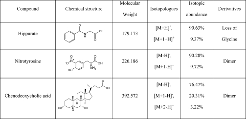
The distribution of the x²_(M) statistics was examined for hippurate, nitrotyrosine, and chenodeoxycholic acid, as well as their respective derivatives (see Table 1). For chenodeoxycholic acid and its dimer, the three lowest mass isotopologues produced signals of sufficient strength for them to be included in the analysis; for the remaining compounds only the two lowest mass isotopologues were included.

Table 1. The Three Compounds Used in the Validation of the Confidence Regions.

Since the construction of the confidence regions requires that the chromatographic peaks used be pure (or comprised only of isomers), continuum plots of all the peaks used were closely inspected. No evidence of contamination was found, and while this cannot guarantee that the peaks are pure, any interference from compounds that are not isomers would tend to inflate the resulting x² statistics, which would lead us to trim a larger proportion of the x² statistics, thus reducing the statistical power of the test. This validation procedure is therefore quite conservative.

To reduce the effects of detector saturation, Coates’s dead time correction algorithm(18) was applied to the continuum data. In addition, the chromatographic scans for which the sum of the corrected ion counts were greater than 300 were removed. Chromatographic scans for which the ion counts were too low, that is, np_i< 5 for some i, were pooled together before the x² statistics were calculated. To obtain a relatively unbiased sampling from the multinomials, all related isotopologues were centroided over an identical number of mass bins.

Validation

To evaluate the degree to which the x² statistics derived from the scans adhere to the appropriate χ² distribution, they were sorted and plotted against the theoretical quantiles of the corresponding χ² distributions. Any substantial departures from the 45° line on the resulting quantile−quantile plots would be indicative of deviations from the predicted distributions. The x² statistics derived from hippurate and nitrotyrosine and their derivatives should all adhere to the χ² distribution with one degree of freedom, since they were derived from two isotopologues. Similarly, the statistics derived from chenodeoxycholic acid and its dimer should all adhere to the χ² distribution with two degrees of freedom, since they were derived from three isotopologues.

The quantile−quantile plots of the x² statistics obtained for the three compounds are shown in Figure 1. The distribution of the statistics obtained from chenodeoxycholic acid appears to be consistent with the χ²₂ distribution. The distributions of the statistics obtained from both hippurate and nitrotyrosine closely approximate the χ²₁ distribution over much of its central range, but have substantially heavier tails as evidenced by the most extreme x² statistics, which render the quantile−quantile plots slightly “flatter” than would be expected for χ²₁-distributed data.

Figure 1.

Quantile−quantile plots of the x² statistics obtained from the three compounds against the appropriate χ² distributions. The red line indicates the idealized fit that would be obtained if the observed x² statistics coincided exactly with the theoretical quantiles of the χ² distributions. While the observed fit is very good for low quantiles, it is clear that the tails of the distributions obtained for hippurate and nitrotyrosine are too heavy to be consistent with that of the χ²₁ distribution.

It is possible that the deviations from the χ²₁ distributions could be explained by mild contaminations from unrelated compounds that were not visible on the continuum plots or by deviations from the standard natural isotopic abundances. However, a more likely explanation is that the tails of the mass peaks of adjacent isotopologues of the same molecular species are heavy enough to have been included in the centroiding, thus distorting the isotopic ratios. Figure 2 shows a continuum plot of the two lowest mass isotopologues of nitrotyrosine, where this phenomenon is clearly visible.

Figure 2.

Continuum plot of the two lowest mass isotopologues of nitrotyrosine. The tails of the mass peaks are heavy enough to reach the apexes of the mass peaks of adjacent isotopologues, so that it is not possible to construct a centroid that is comprised of only one species of isotopologue. While the effect is less apparent for chromatographic scans where the total ion count is lower, the mass peaks at these scans will be all the more sensitive to any contamination.

To account for the effects of the heavy tails, the robust procedure described in the Theory section was applied to the data. When T = 0.05 so that the largest 5% of the x² statistics obtained from the individual scans were removed, the quantile−quantile plots of the resulting distributions displayed tails that were slightly lighter than that of the χ²₁ distribution. However, to ensure that a cautious approach was taken, the value of T = 0.10 was used. The quantile−quantile plots of the resulting distributions are shown in Figure 3.

Figure 3.

Quantile−quantile plots of the x² statistics obtained from the three compounds after the most extreme 10% have been trimmed. The quantiles obtained for hippurate and nitrotyrosine are now consistently smaller than those of the χ²₁ distribution, as required. The effects are more moderate for the x² statistics obtained from chenodeoxycholic acid due to the smaller sample size.

As evidenced by the steep trends on their plots, the tails of the distributions of the x² statistics obtained from hippurate and nitrotyrosine are now considerably lighter than that of the χ²₁ distribution. While the value of T = 0.10 is more than sufficient for all of the compounds that we have investigated, different mass spectrometers operating under different conditions and with different settings might produce mass peaks with heavier tails than we have encountered. Thus, any analyst employing the technique should apply it to known compounds to ensure that the chosen value of T makes the test sufficiently conservative.

We note that, for the test(11) proposed by the authors, for identifying related parent−fragment pairs, which also involved rather similar x² statistics, no trimming was necessary as the x² statistics adhered closely to the appropriate χ² distribution. A key difference between the two methods is that the test for the identification of parent−fragment pairs required the ρ_i in the expression for x² to be estimated from the acquired data, rather than calculated from a theoretical model. It therefore has a degree of flexibility that the current technique does not, and we believe this explains why the latter shows greater sensitivity to the heavy tails of the mass peaks.

Discussion

As mentioned earlier, the practical procedure for formula elucidation, using the confidence regions described above, involves calculating the X² statistic for all chemically realistic formulas that are consistent with the mass error of the mass spectrometer. This was done for hippurate, nitrotyrosine, and chenodeoxycholic acid. The robust procedure for which the 10% most extreme statistics were discarded was applied. The set of chemically realistic formulas was extracted from a list(12) compiled by the Fiehn group, which includes all formulas comprised of C, H, S, N, O, and P, which are consistent with the Lewis rule.

It is difficult to determine the range of chemical formulas that are consistent with a mass estimate obtained through TOF-MS since the uncertainty associated with such estimates is not very well quantified. Modern TOF mass spectrometers are often said to have an accuracy of around 5 ppm; however, to our knowledge, no serious attempt has been made at devising a method for constructing proper confidence intervals for them, although such a procedure would clearly be extremely valuable. While it is true that TOF mass spectrometers are capable of routinely producing mass estimates within 5 ppm of the theoretical mass, this is dependent on having carefully controlled operating conditions, which, in practice, cannot be ensured for all of the compounds encountered in high-throughput LC/MS experiments. Thus, mass errors substantially higher than 5 ppm are possible.

Therefore, to obtain a quite conservative list of candidate formulas, all chemically realistic compounds within 30 ppm of the theoretical masses of the compounds investigated were regarded as being consistent with the mass error of the mass spectrometer. To provide a broader illustration of the ability of the isotopic confidence regions to rule out putative formulas, a second list of all realistic chemical formulas within 0.1 Da of the theoretical masses was also compiled.

In an effort to assess the degree to which a standard chromatographic scan provides information regarding the isotopic abundance pattern, the p-value associated with the median x² statistics, after trimming, of each of the candidate formulas was calculated. Similarly, the median X² statistics derived from the full chromatographic peaks of both the parent compounds and their respective derivatives were calculated. The results are shown in Figure 4.

Figure 4.

Using the robust approach, the median x² and X² statistics were evaluated for the data obtained from hippurate, nitrotyrosine, and chenodeoxycholic acid. The statistics were calculated for all formulas within 0.1 Da of the theoretical mass (black), for all formulas within 30 ppm of the theoretical mass (green), and for the true formula (magenta). Above each plot is listed the number of formulas that may be rejected at the 5% significance level (red line) out of the list of formulas within 30 ppm of the theoretical mass.

It is very clear that, despite the conservative nature of the robust confidence region, it remains a powerful tool for excluding candidate formulas. While the confidence regions constructed from a single scan range from being incapable of rejecting a single formula, in the case of nitrotyrosine, to being capable of rejecting 12, for chenodeoxycholic acid, the confidence regions constructed from the pooled data sets all exclude a substantial number of formulas. Especially in the case of nitrotyrosine, where the proportion of candidate formulas that can be rejected rises from zero to around two-thirds, the benefit of pooling the data is impressive. For the wider mass window of ±0.1 Da the percentage of false candidate formulas that are rejected for all three compounds is 26.79% for the single scan and 70.27% for the pooled data.

Future Prospects

It may be worth investigating the upper limits of what might be achieved if instrumental developments allowed us to sample from undistorted multinomials corresponding to the isotopic abundance patterns. In this scenario we may pool the multinomial counts across the chromatographic peaks, as described in the Theory section, so that we can construct confidence regions on the basis of the outcome of a single multinomial with a very large number of trials. Chromatographic peaks for which detector saturation effects are relatively minor may easily be comprised of 10 000 ion counts under standard operational settings. More intense peaks for which the high ion counts induce significant detector saturation may be comprised of over 100 000 ion counts.

A total of 401 compounds ranging in nominal mass from 100 to 500 and all spaced close to 1 Da apart were extracted from the list of chemically realistic compounds. For each of these, all compounds within 30 ppm of the theoretical masses were considered to be consistent with the mass estimate. A total of 10 000 multinomials corresponding to the isotopic abundance patterns of the selected compounds were simulated. Confidence regions were constructed for each of these simulations, and the mean number of false candidate formulas within these regions was calculated when a significance level of 0.05 was used.

The scenario in which a total of 10 000 counts were obtained was investigated when using either the two or the three lowest mass isotopologues. A more idealized scenario in which a count of 100 000 was obtained was also investigated for the three lowest mass isotopologues. In addition, the number of false negatives obtained when using only the mass estimate was calculated. The results, shown in Figure 5, demonstrate that, as anticipated, the strong statistical power achieved through the high ion counts allows for a very substantial reduction in the number of false candidate formulas when isotopic information is exploited. The statistical power achieved in the scenario in which 100 000 ions are counted is especially impressive, and it should be noted that, at such high counts, it will usually be possible to use more than 3 isotopologues.

Figure 5.

Mean number of false candidate formulas within the confidence regions (false negatives) obtained from the simulated isotopic abundance patterns. The probability that a true candidate formula lies outside a given confidence region (a false positive) is given by the chosen significance level, which was set to 0.05 for these simulations.

Undoubtedly, the assumptions on which the simulations are based are currently highly idealized. However, they clearly suggest that the potential utility of isotopic abundance estimates could be very considerable. Moreover, even without further instrumental developments, it is entirely possible that careful modeling of the detailed characteristics of the mass peaks and of the detection system might allow us to better account for some of the phenomena that currently impede the analysis and thereby obtain substantially improved estimates of the isotopic abundance patterns.

At the high counts used in the above simulations, it is quite possible that the deviations from the standard values of the natural isotopic abundances could confound the analysis. However, we may assume, for simplicity, that the standard abundances had been confirmed in advance, through separate measurements. This supposes a relatively uniform distribution of abundances across the entire sample, but if this assumption is false, the results might be even more interesting. Since different biological reactions can occur at different rates for different isotopologues,(21) they tend to leave a weak isotopic signature on the compounds involved. It is conceivable that potentially very interesting lines of research might be opened if isotopic abundance patterns could be estimated with sufficient accuracy to allow for the detection of these signatures for individual species of molecules.

Conclusion

The above analysis suggests that Pearson’s χ² test provides a reliable method for constructing conservative confidence regions for the isotopic abundance patterns observed in LC/MS experiments. Thus, it is possible to determine, in a statistically rigorous manner, whether the theoretical isotopic abundance pattern of a given chemical formula is consistent with the observed data and thereby reduce the number of candidate formulas for unknown compounds. This is a substantial improvement over alternative methods which attempt only to rank the fit of candidate formulas^13–15 or assume, rather imprecisely, that isotopic abundance estimates are accurate to within a few percent.(12) The method easily allows for information to be pooled from distinct chromatographic scans and from distinct derivatives of the same underlying metabolite.

The method is based on the assumption that the ion counts are Poisson-distributed and therefore does not apply to chromatographic scans for which the ion counts are high enough to induce significant detector saturation. This constraint reduces the power of the test, but it does not affect its validity since even very large chromatographic peaks, which are severely saturated near their apexes, will have low ion counts near their edges, to which the test can be applied. Moreover, the fact that information from distinct scans and distinct derivatives of the same underlying metabolite may be pooled has the effect of increasing the power of the test.

A more serious constraint stems from the fact that there appears to be a certain degree of mixture of the mass peaks of adjacent isotopologues. While the effect is often minor, it necessitates the use of robust methods, if a rigorous statistical argument is to be used in declaring candidate formulas to be inconsistent with the observed data. Again, the consequence is reduced statistical power, although, as was demonstrated, the test remains capable of excluding a substantial number of false candidate formulas.

A fundamental requirement of the test is that the detector used must employ a TDC. While it seems quite possible that confidence regions may also be constructed for mass spectrometers employing ADCs, the procedure may not prove to be as straightforward as for TDCs as it is the ability of the latter to block out electronic noise and preserve the Poisson distribution of incoming ions that makes the procedure particularly simple. Thus, while TDCs are criticized for their relatively limited dynamic range, their ability to produce data that approximate a simple and well-understood distribution constitutes an important advantage.

The application of the test to the three compounds investigated suggests that the information contained in the observed isotopic abundance patterns may be extremely valuable in identifying unknown metabolites, even when these do not contain bromine or chlorine. While we have outlined methods for reducing the size of the confidence regions, it is likely that these might be reduced much further if the information from the chromatographic scans with high ion counts could be included in the analysis or if the mixture of the mass peaks of adjacent isotopologues did not arise. Thus, it is clear that there is scope for improvements in the accuracy with which isotopic abundance patterns can be estimated, and such improvements may be just as important as improvements in mass accuracy. Considering the very high cost of mass spectrometers capable of high mass accuracy, this line of research is, in our view, somewhat neglected.

While the excellent sensitivity of the LC/TOFMS platform has helped to establish it as one of the most predominant analytical tools in metabolomics, the data produced are widely regarded as being of quite variable quality, especially when compared with those obtained through NMR. It is quite possible that this drawback might be overcome if further efforts were made at developing a detailed and comprehensive understanding of the data generated through LC/TOFMS. A method for quantifying the uncertainty associated with the measurements made, as has been presented in this paper, constitutes a small step in this direction. A more ambitious goal would involve a detailed characterization of the underlying mass and chromatographic peaks and of the detector system. This would facilitate further rigor in the data analysis, which may broaden the range of inferences that can be drawn from carrying out a given experiment and strengthen the certainty with which they can be made. In this sense, further developments in the underlying theory of mass spectrometry may be as valuable as developments in instrumentation.

References

- Raamsdonk L. M.; Teusink B.; Broadhurst D.; Zhang N. S.; Hayes A.; Walsh M. C.; Berden J. A.; Brindle K. M.; Kell D. B.; Rowland J. J.; Westerhoff H. V.; van Dam K.; Oliver S. G. Nat. Biotechnol. 2001, 19, 45–50. [DOI] [PubMed] [Google Scholar]
- Want E. J.; O’Maille G.; Smith C. A.; Brandon T. R.; Uritboonthai W.; Qin C.; Trauger S. A.; Siuzdak G. Anal. Chem. 2006, 78, 743–752. [DOI] [PubMed] [Google Scholar]
- Want E. J.; Cravatt B. F.; Siuzdak G. ChemBioChem 2005, 6, 1941–1951. [DOI] [PubMed] [Google Scholar]
- Sleno L.; Volmer D. A.; Marshall A. G. J. Am. Soc. Mass Spectrom. 2005, 16, 183–198. [DOI] [PubMed] [Google Scholar]
- Kind T.; Fiehn O. BMC Bioinf. 2007, 8, 105. [DOI] [PMC free article] [PubMed] [Google Scholar]
- Wu Q. Anal. Chem. 1998, 70, 865–872. [DOI] [PubMed] [Google Scholar]
- Clarke N. J.; Rindgen D.; Korfmacher W. A.; Cox K. A. Anal. Chem. 2001, 73 (15), 430–439. [DOI] [PubMed] [Google Scholar]
- Plumb R.; Johnson K. A.; Rainville P.; Smith B. W.; Wilson I. D.; Castro-Perez J. M.; Nicholson J. K. Rapid Commun. Mass Spectrom. 2006, 20 (13), 1989–1994. [DOI] [PubMed] [Google Scholar]
- Tautenhahn R.; Bottcher C.; Neumann S.. Bioinformatics Research and Development; Lecture Notes in Computer Science; Springer: Heidelberg, Germany, 2007; pp 371−380. [Google Scholar]
- Geromanos S. J.; Silva J. C.; Li G.-Z.; Gorenstein M. V. U.S. Patent Application No. US 2008/0272292, 2008.
- Ipsen A.; Want E. J.; Lindon J. C.; Ebbels T. M. D. Anal. Chem. 2010, 82, 1766–1778. [DOI] [PMC free article] [PubMed] [Google Scholar]
- Kind T.; Fiehn O. BMC Bioinf. 2006, 7, 234. [DOI] [PMC free article] [PubMed] [Google Scholar]
- Böcker S.; Letzel M. C.; Liptákand Z.; Pervukhin A. Bioinformatics 2009, 25 (2), 218–224. [DOI] [PMC free article] [PubMed] [Google Scholar]
- Tong H.; Bell D.; Tabei K.; Siegel M. M. J. Am. Soc. Mass Spectrom. 1999, 10, 1174–1187. [Google Scholar]
- Zhang J. F.; Gao W.; Cai J. J.; He S. M.; Zeng R.; Chen R. S. IEEE/ACM Trans. Comput. Biol. Bioinf. 2005, 2 (3), 217–230. [DOI] [PubMed] [Google Scholar]
- Chernushevich I. V.; Loboda A. V.; Thomson B. A. J. Mass Spectrom. 2001, 36 (8), 849–865. [DOI] [PubMed] [Google Scholar]
- Bateman R. H.; Brown J. M.; Green M.; Wildgoose J. L. International Patent WO 2006/129094, 2006.
- Coates P. Rev. Sci. Instrum. 1991, 63 (3), 2084–2088. [Google Scholar]
- May W. L.; Johnson W. D. Commun. Stat. Simul. Comput. 1997, 26 (2), 495–518. [Google Scholar]
- Bohlke J. K.; de Laeter J. R.; De Bievre P.; Hidaka H.; Peiser H.; Rosman K. J. R.; Taylor P. D. P. J. Phys. Chem. Ref. Data 2005, 34 (1), 57–67. [Google Scholar]
- Gannes L. Z.; del Rio C. M.; Koch P. Comp. Biochem. Physiol. 1998, 119A (3), 725–737. [DOI] [PubMed] [Google Scholar]