Modeling the Hydration Layer around Proteins: HyPred

Abstract

Protein hydration plays an integral role in determining protein function and stability. We develop a simple method with atomic level precision for predicting the solvent density near the surface of a protein. A set of proximal radial distribution functions are defined and calculated for a series of different atom types in proteins using all-atom, explicit solvent molecular dynamic simulations for three globular proteins. A major improvement in predicting the hydration layer is found when the protein is held immobile during the simulations. The distribution functions are used to develop a model for predicting the hydration layer with sub-1-Ångstrom resolution without the need for additional simulations. The model and the distribution functions for a given protein are tested in their ability to reproduce the hydration layer from the simulations for that protein, as well as those for other proteins and for simulations in which the protein atoms are mobile. Predictions for the density of water in the hydration shells are then compared with high occupancy sites observed in crystal structures. The accuracy of both tests demonstrates that the solvation model provides a basis for quantitatively understanding protein solvation and thereby predicting the hydration layer without additional simulations.

Introduction

The solvent affects the thermodynamics and kinetics of numerous biological processes, including protein and nucleic acid folding, stability (1,2) and dynamics (3), enzymology, including transition state stabilization (4), binding (5,6), diffusion, electrostatic interactions (7), charge transfer reactions, ion channel and membrane transporter conductance (8), etc. It is difficult to conceive of a biological process that is independent of solvation. In addition, the presence of a hydration layer surrounding proteins influences many biophysical measurements, including NMR spectroscopy (9–11), x-ray crystallography (12,13), small and wide angle x-ray scattering (SWAXS) (14), and neutron diffraction (15,16). The interpretation of data from all these applications would benefit by having a rapid and accurate model to predict the solvent density around biomolecules. Moreover, the model would provide a fundamental physical basis for describing solvent-biomolecule interactions.

The hydration model we advance here extends and refines the strategy of Pettitt and co-workers (17–20) of using molecular dynamics (MD) simulation data to predict the hydration shell densities surrounding proteins and DNA. The hydration layers deduced from the simulations are converted to a set of electron proximal radial distribution functions (pRDFs) for different atoms types (e.g., N, C, and O). Our goal is to describe the electron density of the hydration shell to calculate the x-ray scattering intensity, which will be discussed in a future article. Given the resolution required, the electrons can be taken to be located, for simplicity, at the nuclear positions. These distribution functions describe the solvent electron density at a position located at a distance r from the closest solute atom which has the designation of atom type a. Subsequent inversion of this mapping process generates a predicted hydration shell density around a protein. This methodology provides the important possibility of predicting the hydration layer of any soluble protein without additional MD simulations.

We address an apparently minor deficiency of Pettitt and co-workers' approach and find a substantial improvement in the prediction of the hydration layer. Our MD simulations maintain the protein atoms immobile, and only the water molecules are allowed to move, whereas their protein is mobile. Additionally, their procedure only specifies different pRDFs for a few distinct atom types, specifically, one each for the O, N and C atoms, while ignoring all solute hydrogen atoms (17). Nevertheless, they have recognized the benefit of calculating the pRDFs for additional atom types (19), and have used many atom types when examining DNA (21). We include the solute hydrogen atoms and further categorize the atoms into subclasses (22) depending on the individual position within each amino acid to generate a total of ∼300 distinct pRDFs (Table S1 in the Supporting Material). Other improvements in our study include the use of longer simulations and finer grid spacing to achieve higher resolution (0.5 vs. 2 Å). Finally, we demonstrate the transferability of the pRDFs by predicting the hydration shell density of a protein using pRDFs from simulations for other proteins. This result indicates the existence of a universal set of pRDFs for describing the hydration layer around globular proteins. Further tests involve the comparison of the predicted hydration layers with those observed in x-ray crystal structures and with simulations in which all protein atoms move.

Molecular Dynamics Simulations

All-atom explicit solvent MD simulations have been performed at the temperature of 4°C for ubiquitin (Ub) (1UBQ (23), 6 ns), hen egg-white lysozyme (HEWL) (6LYZ (24), 3 ns), and myoglobin (Mb) (1WLA (25), 6 ns), employing NAMD (26) and the CHARMM 27 all-atom force field (27). The proteins are solvated in a rectangular periodic box containing rigid TIP3P water molecules (28) and having dimensions 108 × 91 × 104 ų for Ub, 126 × 110 × 104 ų for lysozyme, and 112 × 120 × 99 Å³ for Mb. The ample simulation box dimensions are chosen for future applications (comparisons with SWAXS experiments) and are truncated at 10 Å from the protein's surface to speed up the calculations. Counterions are added to compensate for the charges on the proteins. The solvent for the Ub simulation consists of seven hydrogen phosphate ions, seven dihydrogen phosphate ions, 21 sodium ions, and 33,976 TIP3P water molecules. HEWL is solvated by a solution with 16 acetate ions, eight sodium ions, and 47,470 TIP3P water molecules. The Mb buffer contains five hydrogen phosphate ions, five dihydrogen phosphate ions, and 43,828 TIP3P water molecules.

Energy minimization and equilibration proceeds in several stages. The solvent and protein hydrogen atoms are first energy-minimized for 2000 steps. Then, with the heavy atoms in the protein fixed in place, the temperature of each system begins at 1200 K, and the systems are cooled to 4°C over a period of 100 ps; the systems are then equilibrated for 100 ps at 4°C. The hydrogen atoms in the protein are fixed in place, and the systems are equilibrated for another 100 ps. All protein atoms remain immobile throughout the course of the subsequent simulation to render the comparison of the reconstructed density to the density of MD simulation more meaningful, and an additional simulation of 3 ns of Ub allows motion of all protein atoms. Electrostatic interactions are computed with particle-mesh Ewald summations. A 1-fs time step is used, and snapshots are saved every 1 ps. The simulation uses NVT conditions.

Modeling the density from MD simulations

We evaluate solvent densities in the first few hydration layers and use these densities to generate a model for hydrated proteins without the need for running additional computationally expensive MD simulations. The model is constructed from the average over the MD simulation of the solvent's electron density profile surrounding the protein. Fig. 1, a and c, illustrates the method of calculating the pRDFs. The density is evaluated at 1-ps intervals for every (0.5 Å)³ cube situated outside the protein. Each cube exterior to the protein is assigned to an atom on the protein surface whose scaled van der Waals surface is closest to the center of the cube. An important difference between Pettitt's work and the work presented here is that here the distance to the scaled van der Waals surface is used instead of the distance to the nucleus of the atom. The importance of this feature can be seen by considering a point that is within the van der Waals radius of a large atom but resides closer to outside of the van der Waals radius of a smaller atom. Pettitt's method would predict the cube to contain some solvent density even though the space is insufficient for housing a solvent molecule. Thus, the new approach improves the density reconstruction exterior to the van der Waals radii. Because all protein atoms remain stationary during the simulations, the assignment of cubes to protein atoms only needs specification once at the beginning of the analysis.

Figure 1.

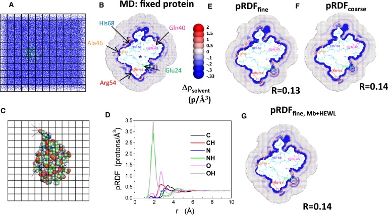
Calculating solvent density around Ub using pRDFs. (A and B) The average solvent density around Ub is obtained from MD simulations with the protein atoms fixed. An 8 Å grid spacing is shown in panels A and C, but 0.5 Å is used in the calculations. Density is defined as protons per ų. (C and D) Using these data, the pRDFs are calculated by identifying the nearest solute atom and distance to each grid element; for example, the oxygen atom (red, upper left) is the closest solute atom to four grid elements (denoted with lines). (E and F) Solvent density calculated by reversing the mapping protocol using the pRDF calculated for the fine and coarse atom type definitions. R-values are listed. The color scale is asymmetric, and hence, noise tends to make the bulk solution appear blue. (G) Solvent density calculated using the averaged pRDFs obtained from Mb and HEWL using the fine atom-type definition. Only one cross-sectional layer of cubes is shown but protein atoms within 3 Å of the layer are displayed. Thus, some proteins atoms can be seen above the slab. Note p = electrons.

Protein atoms are grouped into classes using two different categorizations of atom types to test the degree of specification required for accurate reconstruction of the hydration layer. One specification collects heavy atoms into groups according to their element type (e.g., C, N, O, S…), while hydrogen atoms are grouped together depending on the atom to which they are bonded (e.g., CH, NH, OH…). The other, more detailed specification defines the atom groups according to both their elemental character and amino-acid type. This more detailed set assigns each unique atom in each amino acid type as an atom type (Table S1). The detailed set provides another source of improvement over Pettitt et al., who classify atoms only according to the element. When cubes are equidistant from atoms of the same type, the densities of the cubes are averaged according to Eq. 1. Illustrating this process for the atom type CH yields

$$g_{\text{CH}}\left(r\right)=\frac{1}{N}\sum _{i=1}^N{\rho }_i,$$ (1)

where ρ_i is the density of cube C_i, the summation is performed over all cubes that are assigned to H atoms of type CH, the cubes lie at a distance between r − Δr and r + Δr from the protein's H atom, and N is the number of cubes in the summation. This procedure provides g_CH(r), the proximal radial distribution function (pRDF), which can only be obtained by discretizing the simulation box into cubes.

Reconstructing the density directly

The reconstruction of the hydration shell density without additional MD simulations begins with the protein in the absence of water. The protein and surroundings are partitioned into a grid of cubes as in the mean-field approach of the previous subsection. Let r designate the distance between the center of cube i and the closest scaled van der Waals surface, say of atom type a. Each cube i outside of the protein is assigned the density g_a(r) from the pRDF for the given protein atom type a, the separation r, and the atom type closest to the cube's center. The scale factor used for the van der Waals radius (0.53) is optimized by minimizing the sum of the R factors of the three proteins. Densities in cavities are set to zero. Assigning the densities for ubiquitin takes ∼20–50 CPU seconds. Thus, by determining the pRDFs for a single protein or an average for several proteins, the pRDFs can be used to evaluate the solvent electron density for other proteins without the need for additional MD simulations. We call this process of predicting the hydration layer surrounding the protein “HyPred”.

The first test of the method involves reconstructing the hydration shell density of each protein using the pRDFs determined for that protein. Then, the hydration shell of each protein is evaluated with the average of the pRDFs of the other two proteins. When insufficient data are available for constructing the atom type pRDFs, the missing data are replaced by portions of the pRDFs for the less specific classification by the elements.

Crystallographic water molecules are predicted from both the MD simulations and HyPred reconstructions at positions where the solvent density in a (0.5 Å)³ cube is above a threshold, except when another cube with a higher density lies within 2.8 Å (the diameter of a water molecule).

Results and Discussion

Simulations and radial distribution functions

We begin by performing all-atom MD simulations using explicit (TIP3P) solvent (29) for ubiquitin (Ub, 1UBQ (23)), hen egg white lysozyme (HEWL, 6LYZ (24)), and myoglobin (Mb, 1WLA (25)) and by allowing only the solvent molecules to move (Fig. 1 A). The solvent electron density is calculated for individual frames taken every 1 ps and is averaged over 3000–6000 frames. The local solvent density varies, but generally the simulations display a thin depletion layer just outside the protein (blue in Fig. 2 B). The first hydration layer (red) is found ∼1–2 Å from the protein's surface and is followed by a region of reduced solvent density (blue).

Figure 2.

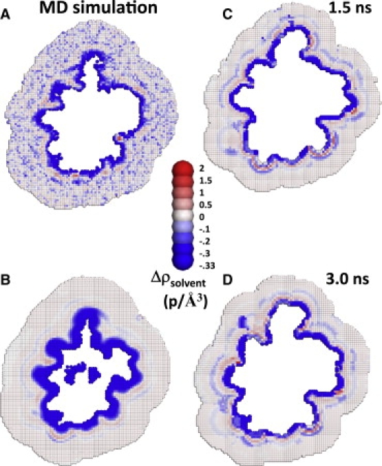
Protein motions affect calculated solvent density. (A) Average solvent density obtained from MD simulations where the protein atoms are allowed to move and (B) the resulting reconstruction. (C and D) Reconstructions for two different protein conformations calculated using pRDFs obtained from the dynamic protein. Note p = electrons.

For comparison, we also calculate the hydration layer when the protein atoms are allowed to move during the simulations (Fig. 2 A). Protein motions, particularly those of surface side chains, can be substantial (e.g., root-mean-squared displacements of 3 Å). Rather than increasing the accuracy of the reconstruction of the hydration layer from a theoretical model, such movement, in fact, artifactually reduces the time-averaged solvent density near the protein as compared to the stationary protein case. For example, a cube might be accessible to water molecules in one snapshot, but could become blocked to solvent in another snapshot due to a side-chain motion. This inaccessibility reduces the average solvent density assigned to the cube, but the decrease is due solely to the physical presence of the side chain and not to an actual repulsion arising from proximity to nearby hydrophobic groups. Hence, permitting protein motions in the MD simulations leads to a gross overestimate of the size and magnitude of the depletion layer at the surface of the protein and thereby impedes the accurate calculation of the reconstructions (Fig. 2). However, when the protein atoms are immobile, a significant but thinner solvent depletion layer remains around the entire protein, and a greater number of regions of high solvent density are observed than when the protein is allowed to move.

The peaks of maximum density in the pRDFs for hydrogens attached to the charged/polar atoms, oxygen and nitrogen, exceed those for hydrogens attached to the more hydrophobic carbon atoms (Fig. 1 D). Similarly, the peak for the oxygen pRDFs is higher than that for carbon. The pRDF for hydrogen atoms bonded to oxygen has the highest peak in the hydrogen category, followed by the pRDF for, hydrogen atoms bonded to nitrogen atoms, and then by the pRDF for oxygen atoms. The pRDF for oxygen exhibits a small peak at 1.8 Å followed by a larger peak at 2.7 Å. The first peak is due to solvent hydrogen atoms, while the second is due to solvent oxygen atoms. The largest peak for the oxygen pRDFs lies further than the first peaks of the pRDFs for hydrogen attached to either oxygen or nitrogen because oxygen has a larger radius than hydrogen and because solute oxygen atoms generally have an intervening hydrogen atom.

Protein atoms are grouped using both coarse and fine definitions to test the degree of specification required to accurately reconstruct the hydration layer. The coarser specification groups heavy atoms by element (C, N, O, and S), with hydrogen atoms grouped according to their bonded heavy atom (CH, NH, OH, and SH). A more refined definition distinguishes between every atom type for each amino acid separately (∼300 types, see Table S1). The utility of the finer definition is evidenced by the fact that pRDFs for O in the coarser definition differ from that for the O_δ of aspartic acid (Fig. 3 A). The difference in accuracy of the hydration layer reconstruction using the two definitions is quantified below.

Figure 3.

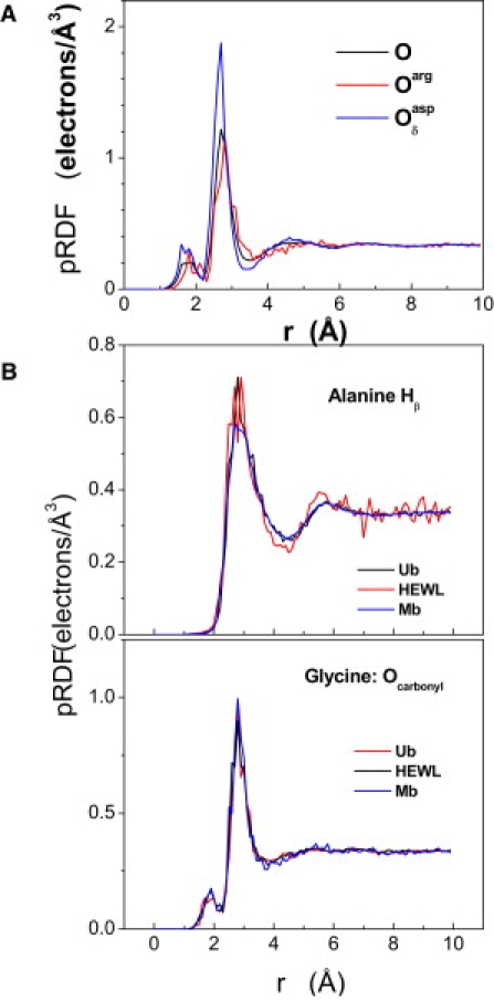
Specificity and transferability of pRDFs. (A) Comparison between coarser and finer definitions of atom types. (B) Comparison among pRDFs calculated from Ub, Mb, and HEWL. The similarity of the pRDFs for the three proteins indicates that the existence of a universal set of pRDFs is applicable to a wide variety of proteins.

The pRDFs calculated from MD simulations for the three proteins are very similar (Fig. 3 B). This identity suggests that pRDFs evaluated for one protein can be used to predict the solvent density around other proteins. This possibility is tested in the next section where the pRDFs determined from one protein are used to predict the hydration shell density simulated for another protein.

Reconstructing the hydration shell: HyPred

This HyPred reconstruction method using the coarser definition of atom types displays fewer features than exhibited using the more refined definition of atom types, and generally the excursions from the average density are reduced (Figs. 1 and 4). The use of the finer definition of pRDFs produces a very similar solvation pattern as the explicit solvent simulations for each of the three proteins. Considering Ub, for example, a region of very high density (red in Fig. 1 B) is present near the hydrogen atoms bonded to the nitrogen atom of the Arg⁵⁴ side chain in both the reconstruction and the MD simulation. Just beyond that high-density region is a regime of very low density that also appears in both the reconstruction and the MD simulation. Generally, very high-density regions tend to be adjacent to regions with very low density.

Figure 4.

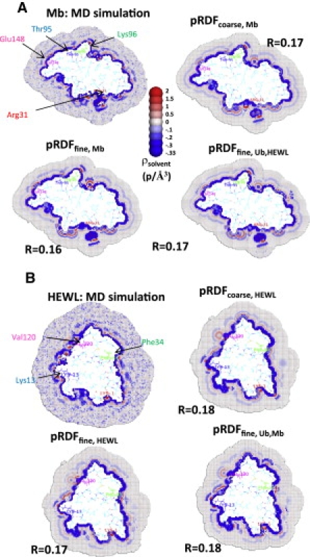
HyPred reconstructions. Solvent density around (A) Mb and (B) HEWL. For each protein, the solvation layer is obtained from either MD simulations or the pRDF derived from the simulations for that protein and for the average of the other two proteins to test for transferability (lower right in panels A and B).

Although most features are well reconstructed, some discrepancies exist. Four high-density regions near Glu²⁴ (green) are present in the MD simulations, but three of these become smeared into a single high-density region in the reconstruction. Another high-density region near Gln⁴⁰ (magenta) appears in both the reconstruction and the MD simulation, although the region is much denser in the simulation, and its accompanying depletion layer has much lower density. Two of the three high-density regions between Ala⁴⁶ (orange) and His⁶⁸ (blue) are well resolved in the reconstruction. The high density near Ala is associated with the amide hydrogen of the backbone nitrogen, demonstrating the importance of performing the reconstruction at the level of individual atoms types. All Ub reconstructions overestimate the density of the depletion layer, separating the first and second hydration layers between Ala⁴⁶ and Arg⁵⁴.

Excellent agreement also is obtained for Mb and HEWL using the finer atom type definition for the pRDFs (Fig. 4). Both the reconstructed and simulated hydration layers for Mb contain a region of very high density followed by a region of very low density near the hydrogen atoms bonded to the nitrogen atoms of Arg³¹ (red). Regions of high density similarly appear near the hydrogen atoms bonded to nitrogen atoms of Lys⁹⁶ (green), near the hydroxyl hydrogen of Thr⁹⁵ (blue), and near Glu¹⁴⁸ (magenta) in both the reconstruction and the MD simulation.

For HEWL, a region of high density near Lys¹ (red) is present in both the reconstruction and MD simulation. Another high-density region near the carbonyl oxygen of Phe³⁴ (green) is evident in the reconstruction and MD simulation, while two high-density regions followed by low-density regions near Lys¹³ (blue) are found in both. Numerous high-density regions between Lys¹³ and Val¹²⁰ appear in the MD simulations but the regions become smeared-out in the reconstruction.

As further demonstration of the importance of calculating the reconstruction using data from MD simulations in which the protein atoms remain stationary, we compare this immobile protein reconstruction to one constructed from simulations in which all the atoms are mobile (Fig. 2). The time-average solvent density surrounding Ub is much more depleted near the protein when Ub is permitted to move during the simulations (Fig. 2, A and B). Two protein snapshots (Fig. 2, C and D) highlight the extent of protein motion and the accompanying change in solvation.

Transferability

The technique presented in this article would be of limited predictive value if it could not enable accurate prediction of the hydration of proteins from the pRDFs determined for other proteins. To check for transferability, the pRDFs obtained from Ub are used to reconstruct the hydration shells around Mb and HEWL. The reconstructions are quite similar to those obtained using their own pRDFs (Fig. 3).

To quantify this agreement between the reconstruction and the MD simulations and any differences resulting from changes in the protocol, three metrics are used (Table 1). The first is the real-space R factor (30),

$$R=\frac{{\sum }_i^N|{\rho }_{o,i}-{\rho }_i|}{{\sum }_i^N|{\rho }_{o,i}+{\rho }_i|},$$

where ρ_o,i is the average solvent density in cube i as calculated from the MD simulation, ρ_i is the reconstructed density for that cube, and the summation runs over cubes that lie within 8 Å of the protein. The second error measure is the RMSD between the two densities (30),

$$RMSD=\frac{\sqrt{N{\sum }_i^N{\left({\rho }_{o,i}-{\rho }_i\right)}^2}}{{\sum }_i^N{\rho }_{o,i}}\text{.}$$

The RMSD weighs more heavily the presence of regions with large disparity between the reconstruction and the MD simulation than the real-space R factor. Because the R factor and RMSD strongly depend upon the extent of the bulk solution that is included in the calculation, we introduce a new measure that is not as strongly dependent upon the amount of bulk solvent in the reconstruction, provided that the simulation is long enough that bulk solvent density fluctuations, i.e., “noise,” is low. This third measure R^∗ is defined as

$$R^{\ast }=\frac{{\sum }_i^N|{\rho }_{o,i}-{\rho }_i|}{{\sum }_i^N|{\rho }_{o,i}+{\rho }_i-2{\rho }_S|},$$

where ρ_s is the bulk solvent density. Bulk solvent should not affect R^∗ significantly because far from the protein, both ρ_o,i and ρ_i should equal ρ_s, and the contribution of the bulk solvent to the numerator and denominator should each vanish.

Table 1.

Accuracy of the density reconstruction at 0.5 Å grid spacing

Protein	pRDF∗	R	RMSD	R∗	pRDF∗	R	RMSD	R∗
Ub	Ub	0.13 (0.14)	0.93 (0.98)	0.43 (0.46)	Mb, HEWL	0.14	0.99	0.46
Mb	Mb	0.16 (0.17)	1.13 (1.17)	0.49 (0.52)	Ub, HEWL	0.17	1.18	0.51
HEWL	HEWL	0.17 (0.18)	1.10 (1.15)	0.51 (0.54)	Ub, Mb	0.18	1.17	0.53

Values in parentheses are for the coarser definition of atom types (C, N, O, S, CH, NH, OH, and SH).

^∗Column indicates the protein(s) whose pRDF is used in reconstruction.

All three metrics confirm that the reconstructions for each of the proteins using the average of the pRDFs of the other two proteins agree well with the reconstruction using the proteins own pRDFs (Table 1). When the pRDFs derived from the MD simulations of HEWL and Mb are averaged together and used to predict the hydration shell of Ub, the reconstruction is only marginally worse than the original obtained using Ub's own pRDFs (R = 0.14 vs. 0.13). These results demonstrate the transferability of the pRDFs to predict the hydration shell of other proteins.

Other factors influencing accuracy

We investigate which other features of our model produce improvements over the methodology of Pettitt and co-workers other than the use of a fixed protein conformation in the MD simulations. These new features include both a finer grid spacing (0.5 vs. 2 Å) and atom type definitions (3 vs. ∼300+), and our separation distance is defined between the cube center and the scaled van der Waals surface rather than to the atom nucleus. The finer grid spacing permits a higher resolution reconstruction. However, the higher resolution has multiple features that degrade the performance as defined by the numerical measures. The 0.5 Å spacing is smaller than the peak widths of the pRDFs. This variation becomes averaged out when using 2 Å cubes, and the predicted map is inferior (Fig. S1). In contrast, the averaging across the 64-fold larger cubes reduces the degree of statistical noise. As a result of the smoothing and the increased statistical accuracy, the R factor and RMSD for Mb decreases from 0.16→0.042 and 1.13→0.22, respectively. The use of larger cubes impacts more on the RMSD because this metric is more sensitive to larger discrepancies. The improved R factor and RMSD of the coarse-grained reconstruction do not imply that the reconstruction is better at a lower resolution; instead, predicting the hydration layer at lower resolution is an easier task.

The improvement in the reconstruction using the finer atom type definition is evident in all three metrics (Table 1). Although the coarser model yields worse results, the data from this model contain reduced noise and thus can be used when insufficient data are available for constructing the pRDF of a specific atom type within some distance range when an unnatural amino acid is present, when an amino acid contains modifications, or for systems other than proteins.

When the separation r in the pRDFs is defined by following the method of Pettitt and co-workers as the distance to the nearest nucleus rather than to the nearest van der Waals surface, the R factor of the reconstruction slightly increases from 0.13 to 0.15 for Ub, 0.16 to 0.18 for Mb, and 0.17 to 0.18 for HEWL. Additional sources of errors may arise from ignoring influences from atoms other than the closest atom and their orientations (e.g., a hydrogen bond has a favored orientation that imparts angular and distance correlations to the local density dependence), from being on a convex versus a concave surface, from the secondary structure of the nearby atoms, and from nearby hydrogen-bond donor/acceptors being internally satisfied versus not being internally satisfied. Despite ignoring all of these details, the HyPred method faithfully reproduces the MD simulations.

Comparison to bound waters in crystal structures

Some attempts at predicting the locations of bound waters have employed information from x-ray crystal structures where highly ordered solvent sites within or near proteins can be identified (31–33). Others have attempted to predict crystallographic waters directly from MD simulations (34,35) and from predictions of hydration shell densities (36). However, only a small number of highly ordered solvent sites can be determined for each protein, and inconsistencies sometimes arise between the sites assigned for different crystal structures of the same protein (37).

Here we test HyPred's ability to predict the positions of high occupancy water molecules in experimental crystal structures. This comparison assumes that crystallographic waters are located at regions of high solvent density in the simulations. A multitude of factors argue against a one-to-one correspondence (16,17), including constraints imposed by crystallographic contacts; differences in temperature and buffer conditions between the simulation and the crystal structures; some assigned crystallographic waters might instead be ions or other solvent molecules; series termination errors may produce ripples that are misidentified as waters; and excess water molecules may be used to over-fit crystallographic data. For example, low temperatures can increase the occupancy in the crystal structures, while the solvent density near charged amino acids is altered by the presence of solvated ions. A study of 10 T4 lysozyme crystal structures finds that 62% of the 20 most frequently occupied water sites are conserved (37). Thus, it is unlikely that any comparison with crystal structures and MD simulations would predict >60% of crystallographic water molecules unless the MD simulation is performed under conditions identical to the experiment. Additionally, a comparison is inherently limited by the accuracy of the underlying MD simulations, which are susceptible to systematic errors due to inaccuracies in the TIP3P water model and the force field.

Nevertheless, we compare water molecules observed in crystallographic structures to regions of high solvent density in both the MD simulations and the HyPred reconstructions. Water molecules are predicted at positions where the solvent density in a (0.5 Å)³ cube is above a threshold level except when another cube with a higher density lies within 2.8 Å (the diameter of a water molecule). Two tests are performed to assess the accuracy.

The first test involves calculating the percentage of the correctly predicted crystallographic water molecules as a function of the total number of predicted water molecules. The number of predicted molecules is varied by adjusting the density threshold. For Ub, Mb, and HEWL, the MD simulations are able to predict between one-quarter and one-half of the crystallographic water molecules, depending on the protein (Fig. 5 A). The HyPred results are slightly worse, but still much better than the control where water molecules are randomly placed within 3 Å of the protein's surface. The accuracy, defined as (true positives)/(total predicted), generally is higher when a higher threshold is used and fewer positions are predicted (Fig. 5 B).

Figure 5.

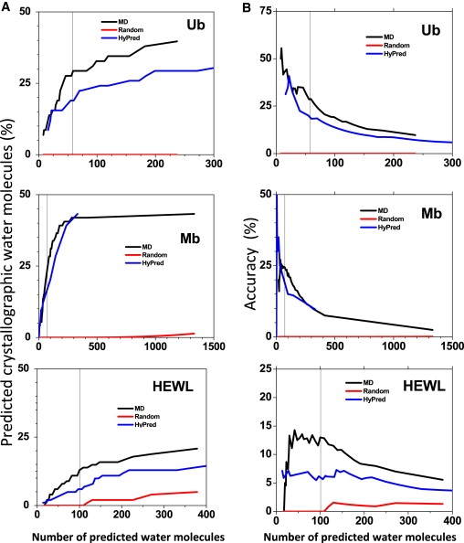
Predicted water molecules around proteins. (A) Using calculations for MD, HyPred, and randomly placed waters within 3 Å of the protein surface, the percentage of crystallographic water molecules with a predicted water molecule within 1 Å is calculated as function of the number of predicted water molecules as the density threshold is progressively decreased (bounded at r < 0.5 electrons/ų). There are 58, 74, and 101 water molecules in the Ub, Mb, and HEWL crystal structures, respectively (vertical black lines).(B) Accuracy, defined as the ratio of the number of crystallographic water molecules correctly predicted relative to the total number predicted, as a function of the total number of predicted water molecules.

In a second test, we calculate the fraction of crystallographic water molecules with a predicted water molecule within a cutoff distance (Fig. S2). The density threshold is adjusted for each protein, so that the same number of water molecules is predicted as observed in its crystallographic structure. When this procedure is performed using the solvent density from the Ub MD simulation, 17 of the 58 waters identified in the crystal structure have a predicted water molecule lying within 1 Å. When the same procedure is performed on the HyPred reconstructed density, 10 of the crystallographic waters have a predicted high occupancy site within 1 Å. Of the 74 crystallographic water molecules in Mb, the MD simulations and HyPred reconstruction correctly predict 18 and 10 molecules within 1 Å, respectively. Of the 101 crystallographic water molecules in HEWL, the MD simulation and HyPred reconstruction correctly predicts 13 and 7 molecules within 1 Å, respectively. For the three proteins, none of the crystallographic waters are nearby the appropriate number of randomly placed water molecules.

Despite the aforementioned caveats concerning the ability of MD simulations to reproduce crystallographic water molecules, these two tests provide experimental support of the validity and utility of the HyPred reconstruction method.

Conclusions

We present a significantly improved model for rapidly calculating the solvent density around a protein. The reconstructions assume that the interactions between the water and protein are well represented by pRDFs for the closest protein atom obtained from MD simulations in which only the water is allowed to move. Radial distributions are found to be independent of protein, thereby enabling the prediction of hydration layers for new proteins without the need for additional MD simulations. A future article will further demonstrate the accuracy of HyPred reconstructions by comparing predicted SWAXS intensities with experiment.

Our use of residue-dependent atom types improves the accuracy of the reconstruction of the hydration layer from the radial distribution functions by implicitly including the influence of nearby side-chain atoms. Improvements might accrue by explicitly incorporating the influence of the second nearest neighbor and other factors, including the local curvature of the protein's van der Waals surface, for hydrogen-bond acceptors or donors; the angle formed between the vector connecting the cube and the protein atom with the vector connecting the atom and the atom to which it is bonded; and using multibody correlation functions. Using the TIP4P or TIP5P water model in the MD simulations might improve agreement with experiment, but that would require the use of a force field optimized for these water models. Future applications include predicting the hydration layer surrounding RNA, DNA, and biological membranes. It might be possible to use a similar method as presented here to predict residence times of water molecules, and the preferred orientations of water molecules around proteins. Additional possibilities involve estimating the free energy of solvation of proteins, with some modifications to a method used by Lazaridis and Paulaitis (39). Eisenberg and McLachlan have calculated solvation free energies based on accessible surface areas (40). The contribution of each atom type to the free energy of solvation could be estimated and compared to solvation parameters of Eisenberg and McLachlan (40).

A website for performing HyPred calculations can be found at http://godzilla.uchicago.edu/cgi-bin/jouko/HyPred.cgi.

References

- 1.Denisov V.P., Jonsson B.H., Halle B. Hydration of denatured and molten globule proteins. Nat. Struct. Biol. 1999;6:253–260. doi: 10.1038/6692. [DOI] [PubMed] [Google Scholar]
- 2.Langhorst U., Backmann J., Steyaert J. Analysis of a water mediated protein-protein interactions within RNase T1. Biochemistry. 2000;39:6586–6593. doi: 10.1021/bi992131m. [DOI] [PubMed] [Google Scholar]
- 3.Tarek M., Tobias D.J. Environmental dependence of the dynamics of protein hydration water. J. Am. Chem. Soc. 1999;121:9740–9741. [Google Scholar]
- 4.Chen C., Beck B.W., Pettitt B.M. Solvent participation in Serratia marcescens endonuclease complexes. Proteins. 2006;62:982–995. doi: 10.1002/prot.20694. [DOI] [PubMed] [Google Scholar]
- 5.Dubins D.N., Filfil R., Chalikian T.V. Role of water in protein-ligand interactions: volumetric characterization of the binding of 2′-CMP and 3′-CMP to ribonuclease A. J. Phys. Chem. B. 2000;104:390–401. [Google Scholar]
- 6.Tame J.R., Sleigh S.H., Ladbury J.E. The role of water in sequence-independent ligand binding by an oligopeptide transporter protein. Nat. Struct. Biol. 1996;3:998–1001. doi: 10.1038/nsb1296-998. [DOI] [PubMed] [Google Scholar]
- 7.Mehl A.F., Demeler B., Zraikat A. A water mediated electrostatic interaction gives thermal stability to the “tail” region of the GrpE protein from E. coli. Protein J. 2007;26:239–245. doi: 10.1007/s10930-006-9065-9. [DOI] [PMC free article] [PubMed] [Google Scholar]
- 8.Yang Y., Berrondo M., Busath D. The importance of water molecules in ion channel simulations. J. Phys. Condens. Matter. 2004;16:S2145–S2148. [Google Scholar]
- 9.Ernst J.A., Clubb R.T., Clore G.M. Demonstration of positionally disordered water within a protein hydrophobic cavity by NMR. Science. 1995;267:1813–1817. doi: 10.1126/science.7892604. [DOI] [PubMed] [Google Scholar]
- 10.Syvitski R.T., Li Y., La Mar G.N. 1H NMR detection of immobilized water molecules within a strong distal hydrogen-bonding network of substrate-bound human heme oxygenase-1. J. Am. Chem. Soc. 2002;124:14296–14297. doi: 10.1021/ja028108x. [DOI] [PubMed] [Google Scholar]
- 11.Tsui V., Radhakrishnan I., Case D.A. NMR and molecular dynamics studies of the hydration of a zinc finger-DNA complex. J. Mol. Biol. 2000;302:1101–1117. doi: 10.1006/jmbi.2000.4108. [DOI] [PubMed] [Google Scholar]
- 12.Higo J., Nakasako M. Hydration structure of human lysozyme investigated by molecular dynamics simulation and cryogenic x-ray crystal structure analyses: on the correlation between crystal water sites, solvent density, and solvent dipole. J. Comput. Chem. 2002;23:1323–1336. doi: 10.1002/jcc.10100. [DOI] [PubMed] [Google Scholar]
- 13.Jiang J.S., Brünger A.T. Protein hydration observed by x-ray diffraction. Solvation properties of penicillopepsin and neuraminidase crystal structures. J. Mol. Biol. 1994;243:100–115. doi: 10.1006/jmbi.1994.1633. [DOI] [PubMed] [Google Scholar]
- 14.Svergun D.I., Richard S., Zaccai G. Protein hydration in solution: experimental observation by x-ray and neutron scattering. Proc. Natl. Acad. Sci. USA. 1998;95:2267–2272. doi: 10.1073/pnas.95.5.2267. [DOI] [PMC free article] [PubMed] [Google Scholar]
- 15.McDowell R.S., Kossiakoff A.A. A comparison of neutron diffraction and molecular dynamics structures: hydroxyl group and water molecule orientations in trypsin. J. Mol. Biol. 1995;250:553–570. doi: 10.1006/jmbi.1995.0397. [DOI] [PubMed] [Google Scholar]
- 16.Savage H., Wlodawer A. Determination of water structure around biomolecules using x-ray and neutron diffraction methods. Methods Enzymol. 1986;127:162–183. doi: 10.1016/0076-6879(86)27014-7. [DOI] [PubMed] [Google Scholar]
- 17.Makarov V., Pettitt B.M., Feig M. Solvation and hydration of proteins and nucleic acids: a theoretical view of simulation and experiment. Acc. Chem. Res. 2002;35:376–384. doi: 10.1021/ar0100273. [DOI] [PubMed] [Google Scholar]
- 18.Feig M., Pettitt B.M. Modeling high-resolution hydration patterns in correlation with DNA sequence and conformation. J. Mol. Biol. 1999;286:1075–1095. doi: 10.1006/jmbi.1998.2486. [DOI] [PubMed] [Google Scholar]
- 19.Lounnas V., Pettitt B.M., Phillips G.N., Jr. A global model of the protein-solvent interface. Biophys. J. 1994;66:601–614. doi: 10.1016/s0006-3495(94)80835-5. [DOI] [PMC free article] [PubMed] [Google Scholar]
- 20.Makarov V.A., Andrews B.K., Pettitt B.M. Reconstructing the protein-water interface. Biopolymers. 1998;45:469–478. doi: 10.1002/(SICI)1097-0282(199806)45:7<469::AID-BIP1>3.0.CO;2-M. [DOI] [PubMed] [Google Scholar]
- 21.Rudnicki W.R., Pettitt B.M. Modeling the DNA-solvent interface. Biopolymers. 1997;41:107–119. doi: 10.1002/(SICI)1097-0282(199701)41:1<107::AID-BIP10>3.0.CO;2-L. [DOI] [PubMed] [Google Scholar]
- 22.Dudowicz J., Freed K.F., Shen M.Y. Hydration structure of Met-encephalin: a molecular dynamics study. J. Chem. Phys. 2003;118:1989–1995. [Google Scholar]
- 23.Vijay-Kumar S., Bugg C.E., Cook W.J. Comparison of the three-dimensional structures of human, yeast, and oat ubiquitin. J. Biol. Chem. 1987;262:6396–6399. [PubMed] [Google Scholar]
- 24.Diamond R. Real-space refinement of the structure of hen egg-white lysozyme. J. Mol. Biol. 1974;82:371–391. doi: 10.1016/0022-2836(74)90598-1. [DOI] [PubMed] [Google Scholar]
- 25.Maurus R., Overall C.M., Brayer G.D. A myoglobin variant with a polar substitution in a conserved hydrophobic cluster in the heme binding pocket. Biochim. Biophys. Acta. 1997;1341:1–13. doi: 10.1016/s0167-4838(97)00064-2. [DOI] [PubMed] [Google Scholar]
- 26.Phillips J.C., Braun R., Schulten K. Scalable molecular dynamics with NAMD. J. Comput. Chem. 2005;26:1781–1802. doi: 10.1002/jcc.20289. [DOI] [PMC free article] [PubMed] [Google Scholar]
- 27.MacKerell A.D., Jr., Bashford D., Karplus M. All-atom empirical potential for molecular modeling and dynamics studies of proteins. J. Phys. Chem. B. 1998;102:3586–3616. doi: 10.1021/jp973084f. [DOI] [PubMed] [Google Scholar]
- 28.Mahoney M.W.J., William L. A five-site model for liquid water and the reproduction of the density anomaly by rigid, nonpolarizable potential functions. J. Chem. Phys. 2000;112:8910–8922. [Google Scholar]
- 29.Jorgensen W.L., Chandrasekhar J., Klein M.L. Comparison of simple potential functions for simulating liquid water. J. Chem. Phys. 1983;79:926–935. [Google Scholar]
- 30.Pettitt B.M., Makarov V.A., Andrews B.K. Protein hydration density: theory, simulations and crystallography. Curr. Opin. Struct. Biol. 1998;8:218–221. doi: 10.1016/s0959-440x(98)80042-0. [DOI] [PubMed] [Google Scholar]
- 31.Schymkowitz J.W., Rousseau F., Serrano L. Prediction of water and metal binding sites and their affinities by using the Fold-X force field. Proc. Natl. Acad. Sci. USA. 2005;102:10147–10152. doi: 10.1073/pnas.0501980102. [DOI] [PMC free article] [PubMed] [Google Scholar]
- 32.Roe S.M., Teeter M.M. Patterns for prediction of hydration around polar residues in proteins. J. Mol. Biol. 1993;229:419–427. doi: 10.1006/jmbi.1993.1043. [DOI] [PubMed] [Google Scholar]
- 33.Schneider B., Cohen D.M., Berman H.M. A systematic method for studying the spatial distribution of water molecules around nucleic acid bases. Biophys. J. 1993;65:2291–2303. doi: 10.1016/S0006-3495(93)81306-7. [DOI] [PMC free article] [PubMed] [Google Scholar]
- 34.Madhusudhan M.S., Vishveshwara S. Deducing hydration sites of a protein from molecular dynamics simulations. J. Biomol. Struct. Dyn. 2001;19:105–114. doi: 10.1080/07391102.2001.10506724. [DOI] [PubMed] [Google Scholar]
- 35.Makarov V.A., Andrews B.K., Pettitt B.M. Residence times of water molecules in the hydration sites of myoglobin. Biophys. J. 2000;79:2966–2974. doi: 10.1016/S0006-3495(00)76533-7. [DOI] [PMC free article] [PubMed] [Google Scholar]
- 36.Hummer G., García A.E., Soumpasis D.M. Hydration of nucleic acid fragments: comparison of theory and experiment for high-resolution crystal structures of RNA, DNA, and DNA-drug complexes. Biophys. J. 1995;68:1639–1652. doi: 10.1016/S0006-3495(95)80381-4. [DOI] [PMC free article] [PubMed] [Google Scholar]
- 37.Zhang X.J., Matthews B.W. Conservation of solvent-binding sites in 10 crystal forms of T4 lysozyme. Protein Sci. 1994;3:1031–1039. doi: 10.1002/pro.5560030705. [DOI] [PMC free article] [PubMed] [Google Scholar]
- 38.Reference deleted in proof.
- 39.Lazaridis T., Paulaitis M.E. Entropy of hydrophobic hydration: a new statistical mechanical formulation. J. Phys. Chem. 1992;96:3847–3855. [Google Scholar]
- 40.Eisenberg D., McLachlan A.D. Solvation energy in protein folding and binding. Nature. 1986;319:199–203. doi: 10.1038/319199a0. [DOI] [PubMed] [Google Scholar]
Associated Data
This section collects any data citations, data availability statements, or supplementary materials included in this article.